数字图像处理论文翻译

中英文资料对照外文翻译一、英文原文A NEW CONTENT BASED MEDIAN FILTERABSTRACTIn this paper the hardware implementation of a contentbased median filter suitabl e for real-time impulse noise suppression is presented. The function of the proposed ci rcuitry is adaptive; it detects the existence of impulse noise in an image neighborhood and applies the median filter operator only when necessary. In this way, the blurring o f the imagein process is avoided and the integrity of edge and detail information is pre served. The proposed digital hardware structure is capable of processing gray-scale im ages of 8-bit resolution and is fully pipelined, whereas parallel processing is used to m inimize computational time. The architecturepresented was implemented in FPGA an d it can be used in industrial imaging applications, where fast processing is of the utm ost importance. The typical system clock frequency is 55 MHz.1. INTRODUCTIONTwo applications of great importance in the area of image processing are noise filtering and image enhancement [1].These tasks are an essential part of any image pro cessor,whether the final image is utilized for visual interpretation or for automatic an alysis. The aim of noise filtering is to eliminate noise and its effects on the original im age, while corrupting the image as little as possible. To this end, nonlinear techniques (like the median and, in general, order statistics filters) have been found to provide mo re satisfactory results in comparison to linear methods. Impulse noise exists in many p ractical applications and can be generated by various sources, including a number of man made phenomena, such as unprotected switches, industrial machines and car ign ition systems. Images are often corrupted by impulse noise due to a noisy sensor or ch annel transmission errors. The most common method used for impulse noise suppressi on n forgray-scale and color images is the median filter (MF) [2].The basic drawback o f the application of the MF is the blurringof the image in process. In the general case,t he filter is applied uniformly across an image, modifying pixels that arenot contamina ted by noise. In this way, the effective elimination of impulse noise is often at the exp ense of an overalldegradation of the image and blurred or distorted features[3].In this paper an intelligent hardware structure of a content based median filter (CBMF) suita ble for impulse noise suppression is presented. The function of the proposed circuit is to detect the existence of noise in the image window and apply the corresponding MFonly when necessary. The noise detection procedure is based on the content of the im age and computes the differences between the central pixel and thesurrounding pixels of a neighborhood. The main advantage of this adaptive approach is that image blurrin g is avoided and the integrity of edge and detail information are preserved[4,5]. The pro posed digital hardware structure is capable of processing gray-scale images of 8-bitres olution and performs both positive and negative impulse noise removal. The architectt ure chosen is based on a sequence of four basic functional pipelined stages, and parall el processing is used within each stage. A moving window of a 3×3 and 5×5-pixel im age neighborhood can be selected. However, the system can be easily expanded to acc ommodate windows of larger sizes. The proposed structure was implemented using fi eld programmable gate arrays (FPGA). The digital circuit was designed, compiled and successfully simulated using the MAX+PLUS II Programmable Logic Development S ystem by Altera Corporation. The EPF10K200SFC484-1 FPGA device of the FLEX1 0KE device family was utilized for the realization of the system. The typical clock fre quency is 55 MHz and the system can be used for real-time imaging applications whe re fast processing is required [6]. As an example,the time required to perform filtering of a gray-scale image of 260×244 pixels is approximately 10.6 msec.2. ADAPTIVE FILTERING PROCEDUREThe output of a median filter at a point x of an image f depends on the values of t he image points in the neighborhood of x. This neighborhood is determined by a wind ow W that is located at point x of f including n points x1, x2, …, xn of f, with n=2k+1. The proposed adaptive content based median filter can be utilized for impulse noisesu p pression in gray-scale images. A block diagram of the adaptive filtering procedure is depicted in Fig. 1. The noise detection procedure for both positive and negative noise is as follows:(i) We consider a neighborhood window W that is located at point x of the image f. Th e differences between the central pixel at point x and the pixel values of the n-1surr ounding points of the neighborhood (excluding thevalue of the central pixel) are co mputed.(ii) The sum of the absolute values of these differences is computed, denoted as fabs(x ). This value provides ameasure of closeness between the central pixel and its su rrounding pixels.(iii) The value fabs(x) is compared to fthreshold(x), which is anappropriately selected positive integer threshold value and can be modified. The central pixel is conside red to be noise when the value fabs(x) is greater than thethreshold value fthresho d(x).(iv) When the central pixel is considered to be noise it is substituted by the median val ue of the image neighborhood,denoted as fk+1, which is the normal operationof the median filter. In the opposite case, the value of the central pixel is not altered and the procedure is repeated for the next neighborhood window.From the noised etection scheme described, it should be mentioned that the noise detection level procedure can be controlled and a range of pixel values (and not only the fixedvalues of 0 and 255, salt and pepper noise) is considered asimpulse noise.In Fig. 2 the results of the application of the median filter and the CBMF in the gray-sca le image “Peppers” are depicted.More specifically, in Fig. 2(a) the original,uncor rupted image“Peppers” is depicted. In Fig. 2(b) the original imagedegraded by 5% both positive and negative impulse noise isillustrated. In Figs 2(c) and 2(d) the resultant images of the application of median filter and CBMF for a 3×3-pixel win dow are shown, respectively. Finally, the resultant images of the application of m edian filter and CBMF for a 5×5-pixelwindow are presented in Figs 2(e) and 2(f). It can be noticed that the application of the CBMF preserves much better edges a nddetails of the images, in comparison to the median filter.A number of different objective measures can be utilized forthe evaluation of these results. The most wi dely used measures are the Mean Square Error (MSE) and the Normalized Mean Square Error (NMSE) [1]. The results of the estimation of these measures for the two filters are depicted in Table I.For the estimation of these measures, the result ant images of the filters are compared to the original, uncorrupted image.From T able I it can be noticed that the MSE and NMSE estimatedfor the application of t he CBMF are considerably smaller than those estimated for the median filter, in all the cases.Table I. Similarity measures.3. HARDWARE ARCHITECTUREThe structure of the adaptive filter comprises four basic functional units, the mo ving window unit , the median computation unit , the arithmetic operations unit , and th e output selection unit . The input data of the system are the gray-scale values of the pi xels of the image neighborhood and the noise threshold value. For the computation of the filter output a3×3 or 5×5-pixel image neighborhood can be selected. Image input d ata is serially imported into the first stage. In this way,the total number of the inputpin s are 24 (21 inputs for the input data and 3 inputs for the clock and the control signalsr equired). The output data of the system are the resultant gray-scale values computed f or the operation selected (8pins).The moving window unit is the internal memory of the system,used for storing th e input values of the pixels and for realizing the moving window operation. The pixel values of the input image, denoted as “IMAGE_INPUT[7..0]”, areimported into this u nit in serial. For the representation of thethreshold value used for the detection of a no Filter Impulse noise 5% mse Nmse(×10-2) 3×3 5×5 3×3 5×5Median CBMF 57.554 35.287 130.496 84.788 0.317 0.194 0.718 0.467ise pixel 13 bits are required. For the moving window operation a 3×3 (5×5)-pixel sep entine type memory is used, consisting of 9 (25)registers. In this way,when the windoP1 P2 P3w is moved into the next image neighborhood only 3 or 5 pixel values stored in the memory are altered. The “en5×5” control signal is used for the selection of the size of th e image window, when“en5×5” is equal to “0” (“1”) a 3×3 (5×5)-pixel neighborhood is selected. It should be mentioned that the modules of the circuit used for the 3×3-pix el window are utilized for the 5×5-pixel window as well. For these modules, 2-to-1mu ltiplexers are utilized to select the appropriate pixel values,where necessary. The mod ules that are utilized only in the case of the 5×5-pixel neighborhood are enabled by th e“en5×5” control signal. The outputs of this unit are rows ofpixel values (3 or 5, respe ctively), which are the inputs to the median computation unit.The task of the median c omputation unit is to compute themedian value of the image neighborhood in order to substitutethe central pixel value, if necessary. For this purpose a25-input sorter is utili zeed. The structure of the sorter has been proposed by Batcher and is based on the use of CS blocks. ACS block is a max/min module; its first output is the maximumof the i nputs and its second output the minimum. The implementation of a CS block includes a comparator and two 2-to-1 multiplexers. The outputs values of the sorter, denoted a s “OUT_0[7..0]”…. “OUT_24[7..0]”, produce a “sorted list” of the 25 initial pixel val ues. A 2-to-1 multiplexer isused for the selection of the median value for a 3×3 or 5×5-pixel neighborhood.The function of the arithmetic operations unit is to computethe value fabs(x), whi ch is compared to the noise threshold value in the final stage of the adaptive filter.The in puts of this unit are the surrounding pixel values and the central pixelof the neighb orhood. For the implementation of the mathematical expression of fabs(x), the circuit of this unit contains a number of adder modules. Note that registers have been used to achieve a pipelined operation. An additional 2-to-1 multiplexer is utilized for the selec tion of the appropriate output value, depending on the “en5×5” control signal. From th e implementation point of view, the use of arithmetic blocks makes this stage hardwar e demanding.The output selection unit is used for the selection of the appropriateoutput value of the performed noise suppression operation. For this selection, the corresponding no ise threshold value calculated for the image neighborhood,“NOISE_THRES HOLD[1 2..0]”,is employed. This value is compared to fabs(x) and the result of the comparison Classifies the central pixel either as impulse noise or not. If thevalue fabs(x) is greater than the threshold value fthreshold(x) the central pixel is positive or negative impulse noise and has to be eliminated. For this reason, the output of the comparison is used as the selection signal of a 2-to-1 multiplexer whose inputs are the central pixel and the c orresponding median value for the image neighborhood. The output of the multiplexer is the output of this stage and the final output of the circuit of the adaptive filter.The st ructure of the CBMF, the computation procedure and the design of the four aforeme n tioned units are illustrated in Fig. 3.ImagewindoeFigure 1: Block diagram of the filtering methodFigure 2: Results of the application of the CBMF: (a) Original image, (b) noise corrupted image (c) Restored image by a 3x3 MF, (d) Restored image by a 3x3 CBMF, (e) Restored image by a 5x5 MF and (f) Restored image by a 5x5 CBMF.4. IMPLEMENTATION ISSUESThe proposed structure was implemented in FPGA,which offer an attractive com bination of low cost, high performance and apparent flexibility, using the software pa ckage+PLUS II of Altera Corporation. The FPGA used is the EPF10K200SFC484-1 d evice of the FLEX10KE device family,a device family suitable for designs that requir e high densities and high I/O count. The 99% of the logic cells(9965/9984 logic cells) of the device was utilized to implement the circuit . The typical operating clock frequ ency of the system is 55 MHz. As a comparison, the time required to perform filtering of a gray-scale image of 260×244 pixelsusing Matlab® software on a Pentium 4/2.4 G Hz computer system is approximately 7.2 sec, whereas the corresponding time using h ardware is approximately 10.6 msec.The modification of the system to accommodate windows oflarger sizes can be done in a straightforward way, requiring onlya small nu mber of changes. More specifically, in the first unit the size of the serpentine memory P4P5P6P7P8P9SubtractorarryMedianfilteradder comparatormuitiplexerf abc(x)valueand the corresponding number of multiplexers increase following a square law. In the second unit, the sorter module should be modified,and in the third unit the number of the adder devicesincreases following a square law. In the last unit no changes are requ ired.5. CONCLUSIONSThis paper presents a new hardware structure of a content based median filter, ca pable of performing adaptive impulse noise removal for gray-scale images. The noise detection procedure takes into account the differences between the central pixel and th e surrounding pixels of a neighborhood.The proposed digital circuit is capable ofproce ssing grayscale images of 8-bit resolution, with 3×3 or 5×5-pixel neighborhoods as op tions for the computation of the filter output. However, the design of the circuit is dire ctly expandableto accommodate larger size image windows. The adaptive filter was d eigned and implemented in FPGA. The typical clock frequency is 55 MHz and the sys tem is suitable forreal-time imaging applications.REFERENCES[1] W. K. Pratt, Digital Image Processing. New York: Wiley,1991.[2] G. R. Arce, N. C. Gallagher and T. Nodes, “Median filters:Theory and applicat ions,” in Advances in ComputerVision and Image Processing, Greenwich, CT: JAI, 1986.[3] T. A. Nodes and N. C. Gallagher, Jr., “The output distributionof median type filte rs,” IEEE Transactions onCommunications, vol. COM-32, pp. 532-541, May1984.[4] T. Sun and Y. Neuvo, “Detail-preserving median basedfilters in imageprocessing,” Pattern Recognition Letters,vol. 15, pp. 341-347, Apr. 1994.[5] E. Abreau, M. Lightstone, S. K. Mitra, and K. Arakawa,“A new efficient approachfor the removal of impulsenoise from highly corrupted images,” IEEE Transa ctionson Image Processing, vol. 5, pp. 1012-1025, June 1996.[6] E. R. Dougherty and P. Laplante, Introduction to Real-Time Imaging, Bellingham:SPIE/IEEE Press, 1995.二、英文翻译基于中值滤波的新的内容摘要在本设计中的提出了基于中值滤波的硬件实现用来抑制脉冲噪声的干扰。

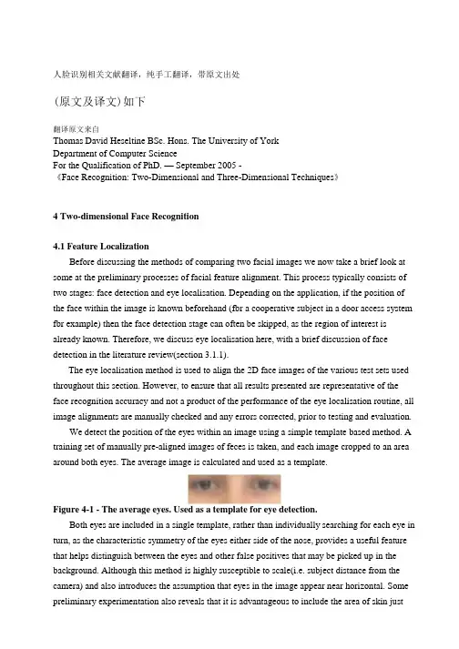
人脸识别相关文献翻译，纯手工翻译，带原文出处(原文及译文)如下翻译原文来自Thomas David Heseltine BSc. Hons. The University of YorkDepartment of Computer ScienceFor the Qualification of PhD. — September 2005 -《Face Recognition: Two-Dimensional and Three-Dimensional Techniques》4 Two-dimensional Face Recognition4.1 Feature LocalizationBefore discussing the methods of comparing two facial images we now take a brief look at some at the preliminary processes of facial feature alignment. This process typically consists of two stages: face detection and eye localisation. Depending on the application, if the position of the face within the image is known beforehand (fbr a cooperative subject in a door access system fbr example) then the face detection stage can often be skipped, as the region of interest is already known. Therefore, we discuss eye localisation here, with a brief discussion of face detection in the literature review(section 3.1.1).The eye localisation method is used to align the 2D face images of the various test sets used throughout this section. However, to ensure that all results presented are representative of the face recognition accuracy and not a product of the performance of the eye localisation routine, all image alignments are manually checked and any errors corrected, prior to testing and evaluation.We detect the position of the eyes within an image using a simple template based method. A training set of manually pre-aligned images of feces is taken, and each image cropped to an area around both eyes. The average image is calculated and used as a template.Figure 4-1 - The average eyes. Used as a template for eye detection.Both eyes are included in a single template, rather than individually searching for each eye in turn, as the characteristic symmetry of the eyes either side of the nose, provides a useful feature that helps distinguish between the eyes and other false positives that may be picked up in the background. Although this method is highly susceptible to scale(i.e. subject distance from the camera) and also introduces the assumption that eyes in the image appear near horizontal. Some preliminary experimentation also reveals that it is advantageous to include the area of skin justbeneath the eyes. The reason being that in some cases the eyebrows can closely match the template, particularly if there are shadows in the eye-sockets, but the area of skin below the eyes helps to distinguish the eyes from eyebrows (the area just below the eyebrows contain eyes, whereas the area below the eyes contains only plain skin).A window is passed over the test images and the absolute difference taken to that of the average eye image shown above. The area of the image with the lowest difference is taken as the region of interest containing the eyes. Applying the same procedure using a smaller template of the individual left and right eyes then refines each eye position.This basic template-based method of eye localisation, although providing fairly preciselocalisations, often fails to locate the eyes completely. However, we are able to improve performance by including a weighting scheme.Eye localisation is performed on the set of training images, which is then separated into two sets: those in which eye detection was successful; and those in which eye detection failed. Taking the set of successful localisations we compute the average distance from the eye template (Figure 4-2 top). Note that the image is quite dark, indicating that the detected eyes correlate closely to the eye template, as we would expect. However, bright points do occur near the whites of the eye, suggesting that this area is often inconsistent, varying greatly from the average eye template.Figure 4-2 一Distance to the eye template for successful detections (top) indicating variance due to noise and failed detections (bottom) showing credible variance due to miss-detected features.In the lower image (Figure 4-2 bottom), we have taken the set of failed localisations(images of the forehead, nose, cheeks, background etc. falsely detected by the localisation routine) and once again computed the average distance from the eye template. The bright pupils surrounded by darker areas indicate that a failed match is often due to the high correlation of the nose and cheekbone regions overwhelming the poorly correlated pupils. Wanting to emphasise the difference of the pupil regions for these failed matches and minimise the variance of the whites of the eyes for successful matches, we divide the lower image values by the upper image to produce a weights vector as shown in Figure 4-3. When applied to the difference image before summing a total error, this weighting scheme provides a much improved detection rate.Figure 4-3 - Eye template weights used to give higher priority to those pixels that best represent the eyes.4.2 The Direct Correlation ApproachWe begin our investigation into face recognition with perhaps the simplest approach,known as the direct correlation method (also referred to as template matching by Brunelli and Poggio [29 ]) involving the direct comparison of pixel intensity values taken from facial images. We use the term "Direct Conelation, to encompass all techniques in which face images are compared directly, without any form of image space analysis, weighting schemes or feature extraction, regardless of the distance metric used. Therefore, we do not infer that Pearson's correlation is applied as the similarity function (although such an approach would obviously come under our definition of direct correlation). We typically use the Euclidean distance as our metric in these investigations (inversely related to Pearson's correlation and can be considered as a scale and translation sensitive form of image correlation), as this persists with the contrast made between image space and subspace approaches in later sections.Firstly, all facial images must be aligned such that the eye centres are located at two specified pixel coordinates and the image cropped to remove any background information. These images are stored as greyscale bitmaps of 65 by 82 pixels and prior to recognition converted into a vector of 5330 elements (each element containing the corresponding pixel intensity value). Each corresponding vector can be thought of as describing a point within a 5330 dimensional image space. This simple principle can easily be extended to much larger images: a 256 by 256 pixel image occupies a single point in 65,536-dimensional image space and again, similar images occupy close points within that space. Likewise, similar faces are located close together within the image space, while dissimilar faces are spaced far apart. Calculating the Euclidean distance d, between two facial image vectors (often referred to as the query image q, and gallery image g), we get an indication of similarity. A threshold is then applied to make the final verification decision.d . q - g ( threshold accept ) (d threshold ⇒ reject ). Equ. 4-14.2.1 Verification TestsThe primary concern in any face recognition system is its ability to correctly verify a claimed identity or determine a person's most likely identity from a set of potential matches in a database. In order to assess a given system's ability to perform these tasks, a variety of evaluation methodologies have arisen. Some of these analysis methods simulate a specific mode of operation (i.e. secure site access or surveillance), while others provide a more mathematicaldescription of data distribution in some classification space. In addition, the results generated from each analysis method may be presented in a variety of formats. Throughout the experimentations in this thesis, we primarily use the verification test as our method of analysis and comparison, although we also use Fisher's Linear Discriminant to analyse individual subspace components in section 7 and the identification test for the final evaluations described in section 8. The verification test measures a system's ability to correctly accept or reject the proposed identity of an individual. At a functional level, this reduces to two images being presented for comparison, fbr which the system must return either an acceptance (the two images are of the same person) or rejection (the two images are of different people). The test is designed to simulate the application area of secure site access. In this scenario, a subject will present some form of identification at a point of entry, perhaps as a swipe card, proximity chip or PIN number. This number is then used to retrieve a stored image from a database of known subjects (often referred to as the target or gallery image) and compared with a live image captured at the point of entry (the query image). Access is then granted depending on the acceptance/rej ection decision.The results of the test are calculated according to how many times the accept/reject decision is made correctly. In order to execute this test we must first define our test set of face images. Although the number of images in the test set does not affect the results produced (as the error rates are specified as percentages of image comparisons), it is important to ensure that the test set is sufficiently large such that statistical anomalies become insignificant (fbr example, a couple of badly aligned images matching well). Also, the type of images (high variation in lighting, partial occlusions etc.) will significantly alter the results of the test. Therefore, in order to compare multiple face recognition systems, they must be applied to the same test set.However, it should also be noted that if the results are to be representative of system performance in a real world situation, then the test data should be captured under precisely the same circumstances as in the application environment.On the other hand, if the purpose of the experimentation is to evaluate and improve a method of face recognition, which may be applied to a range of application environments, then the test data should present the range of difficulties that are to be overcome. This may mean including a greater percentage of6difficult9 images than would be expected in the perceived operating conditions and hence higher error rates in the results produced. Below we provide the algorithm for executing the verification test. The algorithm is applied to a single test set of face images, using a single function call to the face recognition algorithm: CompareF aces(F ace A, FaceB). This call is used to compare two facial images, returning a distance score indicating how dissimilar the two face images are: the lower the score the more similar the two face images. Ideally, images of the same face should produce low scores, while images of different faces should produce high scores.Every image is compared with every other image, no image is compared with itself and nopair is compared more than once (we assume that the relationship is symmetrical). Once two images have been compared, producing a similarity score, the ground-truth is used to determine if the images are of the same person or different people. In practical tests this information is often encapsulated as part of the image filename (by means of a unique person identifier). Scores are then stored in one of two lists: a list containing scores produced by comparing images of different people and a list containing scores produced by comparing images of the same person. The final acceptance/rejection decision is made by application of a threshold. Any incorrect decision is recorded as either a false acceptance or false rejection. The false rejection rate (FRR) is calculated as the percentage of scores from the same people that were classified as rejections. The false acceptance rate (FAR) is calculated as the percentage of scores from different people that were classified as acceptances.For IndexA = 0 to length(TestSet) For IndexB = IndexA+l to length(TestSet) Score = CompareFaces(TestSet[IndexA], TestSet[IndexB]) If IndexA and IndexB are the same person Append Score to AcceptScoresListElseAppend Score to RejectScoresListFor Threshold = Minimum Score to Maximum Score:FalseAcceptCount, FalseRejectCount = 0For each Score in RejectScoresListIf Score <= ThresholdIncrease FalseAcceptCountFor each Score in AcceptScoresListIf Score > ThresholdIncrease FalseRejectCountF alse AcceptRate = FalseAcceptCount / Length(AcceptScoresList)FalseRej ectRate = FalseRejectCount / length(RejectScoresList)Add plot to error curve at (FalseRejectRate, FalseAcceptRate)These two error rates express the inadequacies of the system when operating at aspecific threshold value. Ideally, both these figures should be zero, but in reality reducing either the FAR or FRR (by altering the threshold value) will inevitably resultin increasing the other. Therefore, in order to describe the full operating range of a particular system, we vary the threshold value through the entire range of scores produced. The application of each threshold value produces an additional FAR, FRR pair, which when plotted on a graph produces the error rate curve shown below.False Acceptance Rate / %Figure 4-5 - Example Error Rate Curve produced by the verification test.The equal error rate (EER) can be seen as the point at which FAR is equal to FRR. This EER value is often used as a single figure representing the general recognition performance of a biometric system and allows for easy visual comparison of multiple methods. However, it is important to note that the EER does not indicate the level of error that would be expected in a real world application. It is unlikely that any real system would use a threshold value such that the percentage of false acceptances were equal to the percentage of false rejections. Secure site access systems would typically set the threshold such that false acceptances were significantly lower than false rejections: unwilling to tolerate intruders at the cost of inconvenient access denials.Surveillance systems on the other hand would require low false rejection rates to successfully identify people in a less controlled environment. Therefore we should bear in mind that a system with a lower EER might not necessarily be the better performer towards the extremes of its operating capability.There is a strong connection between the above graph and the receiver operating characteristic (ROC) curves, also used in such experiments. Both graphs are simply two visualisations of the same results, in that the ROC format uses the True Acceptance Rate(TAR), where TAR = 1.0 - FRR in place of the FRR, effectively flipping the graph vertically. Another visualisation of the verification test results is to display both the FRR and FAR as functions of the threshold value. This presentation format provides a reference to determine the threshold value necessary to achieve a specific FRR and FAR. The EER can be seen as the point where the two curves intersect.Figure 4-6 - Example error rate curve as a function of the score threshold The fluctuation of these error curves due to noise and other errors is dependant on the number of face image comparisons made to generate the data. A small dataset that only allows fbr a small number of comparisons will results in a jagged curve, in which large steps correspond to the influence of a single image on a high proportion of the comparisons made. A typical dataset of 720 images (as used in section 4.2.2) provides 258,840 verification operations, hence a drop of 1% EER represents an additional 2588 correct decisions, whereas the quality of a single image could cause the EER to fluctuate by up to 0.28.422 ResultsAs a simple experiment to test the direct correlation method, we apply the technique described above to a test set of 720 images of 60 different people, taken from the AR Face Database [ 39 ]. Every image is compared with every other image in the test set to produce a likeness score, providing 258,840 verification operations from which to calculate false acceptance rates and false rejection rates. The error curve produced is shown in Figure 4-7.Figure 4-7 - Error rate curve produced by the direct correlation method using no image preprocessing.We see that an EER of 25.1% is produced, meaning that at the EER threshold approximately one quarter of all verification operations carried out resulted in an incorrect classification. Thereare a number of well-known reasons for this poor level of accuracy. Tiny changes in lighting, expression or head orientation cause the location in image space to change dramatically. Images in face space are moved far apart due to these image capture conditions, despite being of the same person's face. The distance between images of different people becomes smaller than the area of face space covered by images of the same person and hence false acceptances and false rejections occur frequently. Other disadvantages include the large amount of storage necessaryfor holding many face images and the intensive processing required for each comparison, making this method unsuitable fbr applications applied to a large database. In section 4.3 we explore the eigenface method, which attempts to address some of these issues.4二维人脸识别4.1功能定位在讨论比较两个人脸图像，我们现在就简要介绍的方法一些在人脸特征的初步调整过程。

数字图像处理外文翻译参考文献(文档含中英文对照即英文原文和中文翻译)原文：Application Of Digital Image Processing In The MeasurementOf Casting Surface RoughnessAhstract- This paper presents a surface image acquisition system based on digital image processing technology. The image acquired by CCD is pre-processed through the procedure of image editing, image equalization, the image binary conversation and feature parameters extraction to achieve casting surface roughness measurement. The three-dimensional evaluation method is taken to obtain the evaluation parametersand the casting surface roughness based on feature parameters extraction. An automatic detection interface of casting surface roughness based on MA TLAB is compiled which can provide a solid foundation for the online and fast detection of casting surface roughness based on image processing technology.Keywords-casting surface; roughness measurement; image processing; feature parametersⅠ.INTRODUCTIONNowadays the demand for the quality and surface roughness of machining is highly increased, and the machine vision inspection based on image processing has become one of the hotspot of measuring technology in mechanical industry due to their advantages such as non-contact, fast speed, suitable precision, strong ability of anti-interference, etc [1,2]. As there is no laws about the casting surface and the range of roughness is wide, detection parameters just related to highly direction can not meet the current requirements of the development of the photoelectric technology, horizontal spacing or roughness also requires a quantitative representation. Therefore, the three-dimensional evaluation system of the casting surface roughness is established as the goal [3,4], surface roughness measurement based on image processing technology is presented. Image preprocessing is deduced through the image enhancement processing, the image binary conversation. The three-dimensional roughness evaluation based on the feature parameters is performed . An automatic detection interface of casting surface roughness based on MA TLAB is compiled which provides a solid foundation for the online and fast detection of casting surface roughness.II. CASTING SURFACE IMAGE ACQUISITION SYSTEMThe acquisition system is composed of the sample carrier, microscope, CCD camera, image acquisition card and the computer. Sample carrier is used to place tested castings. According to the experimental requirements, we can select a fixed carrier and the sample location can be manually transformed, or select curing specimens and the position of the sampling stage can be changed. Figure 1 shows the whole processing procedure.,Firstly,the detected castings should be placed in the illuminated backgrounds as far as possible, and then through regulating optical lens, setting the CCD camera resolution and exposure time, the pictures collected by CCD are saved to computer memory through the acquisition card. The image preprocessing and feature value extraction on casting surface based on corresponding software are followed. Finally the detecting result is output.III. CASTING SURFACE IMAGE PROCESSINGCasting surface image processing includes image editing, equalization processing, image enhancement and the image binary conversation,etc. The original and clipped images of the measured casting is given in Figure 2. In which a) presents the original image and b) shows the clipped image.A.Image EnhancementImage enhancement is a kind of processing method which can highlight certain image information according to some specific needs and weaken or remove some unwanted informations at the same time[5].In order to obtain more clearly contour of the casting surface equalization processing of the image namely the correction of the image histogram should be pre-processed before image segmentation processing. Figure 3 shows the original grayscale image and equalization processing image and their histograms. As shown in the figure, each gray level of the histogram has substantially the same pixel point and becomes more flat after gray equalization processing. The image appears more clearly after the correction and the contrast of the image is enhanced.Fig.2 Casting surface imageFig.3 Equalization processing imageB. Image SegmentationImage segmentation is the process of pixel classification in essence. It is a very important technology by threshold classification. The optimal threshold is attained through the instmction thresh = graythresh (II). Figure 4 shows the image of the binary conversation. The gray value of the black areas of the Image displays the portion of the contour less than the threshold (0.43137), while the white area shows the gray value greater than the threshold. The shadows and shading emerge in the bright region may be caused by noise or surface depression.Fig4 Binary conversationIV. ROUGHNESS PARAMETER EXTRACTIONIn order to detect the surface roughness, it is necessary to extract feature parameters of roughness. The average histogram and variance are parameters used to characterize the texture size of surface contour. While unit surface's peak area is parameter that can reflect the roughness of horizontal workpiece.And kurtosis parameter can both characterize the roughness of vertical direction and horizontal direction. Therefore, this paper establisheshistogram of the mean and variance, the unit surface's peak area and the steepness as the roughness evaluating parameters of the castings 3D assessment. Image preprocessing and feature extraction interface is compiled based on MATLAB. Figure 5 shows the detection interface of surface roughness. Image preprocessing of the clipped casting can be successfully achieved by this software, which includes image filtering, image enhancement, image segmentation and histogram equalization, and it can also display the extracted evaluation parameters of surface roughness.Fig.5 Automatic roughness measurement interfaceV. CONCLUSIONSThis paper investigates the casting surface roughness measuring method based on digital Image processing technology. The method is composed of image acquisition, image enhancement, the image binary conversation and the extraction of characteristic parameters of roughness casting surface. The interface of image preprocessing and the extraction of roughness evaluation parameters is compiled by MA TLAB which can provide a solid foundation for the online and fast detection of casting surface roughness.REFERENCE[1] Xu Deyan, Lin Zunqi. The optical surface roughness research pro gress and direction[1]. Optical instruments 1996, 18 (1): 32-37.[2] Wang Yujing. Turning surface roughness based on image measurement [D]. Harbin:Harbin University of Science and Technology[3] BRADLEY C. Automated surface roughness measurement[1]. The InternationalJournal of Advanced Manufacturing Technology ,2000,16(9) :668-674.[4] Li Chenggui, Li xing-shan, Qiang XI-FU 3D surface topography measurement method[J]. Aerospace measurement technology, 2000, 20(4): 2-10.[5] Liu He. Digital image processing and application [ M]. China Electric Power Press,2005译文：数字图像处理在铸件表面粗糙度测量中的应用摘要—本文提出了一种表面图像采集基于数字图像处理技术的系统。

中英文对照外文翻译文献(文档含英文原文和中文翻译)Elastic image matchingAbstractOne fundamental problem in image recognition is to establish the resemblance of two images. This can be done by searching the best pixel to pixel mapping taking into account monotonicity and continuity constraints. We show that this problem is NP-complete by reduction from 3-SAT, thus giving evidence that the known exponential time algorithms are justified, but approximation algorithms or simplifications are necessary.Keywords: Elastic image matching; Two-dimensional warping; NP-completeness 1. IntroductionIn image recognition, a common problem is to match two given images, e.g. when comparing an observed image to given references. In that pro-cess, elastic image matching, two-dimensional (2D-)warping (Uchida and Sakoe, 1998) or similar types of invariant methods (Keysers et al., 2000) can be used. For this purpose, we can define cost functions depending on the distortion introduced in the matching andsearch for the best matching with respect to a given cost function. In this paper, we show that it is an algorithmically hard problem to decide whether a matching between two images exists with costs below a given threshold. We show that the problem image matching is NP-complete by means of a reduction from 3-SAT, which is a common method of demonstrating a problem to be intrinsically hard (Garey and Johnson, 1979). This result shows the inherent computational difficulties in this type of image comparison, while interestingly the same problem is solvable for 1D sequences in polynomial time, e.g. the dynamic time warping problem in speech recognition (see e.g. Ney et al., 1992). This has the following implications: researchers who are interested in an exact solution to this problem cannot hope to find a polynomial time algorithm, unless P=NP. Furthermore, one can conclude that exponential time algorithms as presented and extended by Uchida and Sakoe (1998, 1999a,b, 2000a,b) may be justified for some image matching applications. On the other hand this shows that those interested in faster algorithms––e.g. for pattern recognition purposes––are right in searching for sub-optimal solutions. One method to do this is the restriction to local optimizations or linear approximations of global transformations as presented in (Keysers et al., 2000). Another possibility is to use heuristic approaches like simulated annealing or genetic algorithms to find an approximate solution. Furthermore, methods like beam search are promising candidates, as these are used successfully in speech recognition, although linguistic decoding is also an NP-complete problem (Casacuberta and de la Higuera, 1999). 2. Image matchingAmong the varieties of matching algorithms,we choose the one presented by Uchida and Sakoe(1998) as a starting point to formalize the problem image matching. Let the images be given as(without loss of generality) square grids of size M×M with gray values (respectively node labels)from a finite alphabet &={1，…，G}. To define thed：&×&→N , problem, two distance functions are needed,one acting on gray valuesg measuring the match in gray values, and one acting on displacement differences :Z×Z→N , measuring the distortion introduced by t he matching. For these distance ddfunctions we assume that they are monotonous functions (computable in polynomial time) of the commonly used squared Euclid-ean distance, i.ed g (g 1,g 2)=f 1(||g 1-g 2||²)and d d (z)=f 2(||z||²) monotonously increasing. Now we call the following optimization problem the image matching problem (let µ={1，…M} ).Instance: The pair( A ; B ) of two images A and B of size M×M .Solution: A mapping function f :µ×µ→µ×µ.Measure:c （A,B,f ）=),(),(j i f ij g B Ad ∑μμ⨯∈),(j i+∑⨯-⋅⋅⋅∈+-+μ}1,{1,),()))0,1(),(())0,1(),(((M j i d j i f j i f dμ⨯-⋅⋅⋅∈}1,{1,),(M j i +∑⋅⋅⋅⨯∈+-+1}-M ,{1,),()))1,0(),(())1,0(),(((μj i d j i f j i f d 1}-M ,{1,),(⋅⋅⋅⨯∈μj iGoal:min f c(A,B,f).In other words, the problem is to find the mapping from A onto B that minimizes the distance between the mapped gray values together with a measure for the distortion introduced by the mapping. Here, the distortion is measured by the deviation from the identity mapping in the two dimensions. The identity mapping fulfills f(i,j)=(i,j),and therefore ，f((i,j)+(x,y))=f(i,j)+(x,y)The corresponding decision problem is fixed by the followingQuestion:Given an instance of image matching and a cost c′, does there exist a ma pping f such that c(A,B,f)≤c′?In the definition of the problem some care must be taken concerning the distance functions. For example, if either one of the distance functions is a constant function, the problem is clearly in P (for d g constant, the minimum is given by the identity mapping and for d d constant, the minimum can be determined by sorting all possible matching for each pixel by gray value cost and mapping to one of the pixels with minimum cost). But these special cases are not those we are concerned with in image matching in general.We choose the matching problem of Uchida and Sakoe (1998) to complete the definition of the problem. Here, the mapping functions are restricted by continuity and monotonicity constraints: the deviations from the identity mapping may locally be at most one pixel (i.e. limited to the eight-neighborhood with squared Euclidean distance less than or equal to 2). This can be formalized in this approach bychoosing the functions f1,f2as e.g.f 1=id，f2(x)=step(x):=⎩⎨⎧.2,)10(,2,0>≤⋅xGxMM3. Reduction from 3-SAT3-SAT is a very well-known NP-complete problem (Garey and Johnson, 1979), where 3-SAT is defined as follows:Instance: Collection of clauses C={C1，···,CK} on a set of variables X={x1， (x)L}such that each ckconsists of 3 literals for k=1，···K .Each literal is a variable or the negation of a variable.Question:Is there a truth assignment for X which satisfies each clause ck, k=1，···K ?The dependency graph D（Ф）corresponding to an instance Ф of 3-SAT is defined to be the bipartite graph whose independent sets are formed by the set of clauses Cand the set of variables X .Two vert ices ck and x1are adjacent iff ckinvolvesx 1or-xL.Given any 3-SAT formula U, we show how to construct in polynomial time anequivalent image matching problem l（Ф）=（A(Ф),B(Ф)）; . The two images of l （Ф）are similar according to the cost function （i.e.f:c(A(Ф),B(Ф),f）≤0) iff the formulaФ is satisfiable. We perform the reduction from 3-SAT using the following steps:• From the formula Ф we construct the dependency graph D（Ф）.• The dependency graph D（Ф）is drawn in the plane.• The drawing of D（Ф）is refined to depict the logical behaviour of Ф , yielding two images（A(Ф),B(Ф)）.For this, we use three types of components: one component to represent variables of Ф , one component to represent clauses of Ф, and components which act as interfaces between the former two types. Before we give the formal reduction, we introduce these components.3.1. Basic componentsFor the reduction from 3-SAT we need five components from which we will construct the in-stances for image matching , given a Boolean formula in 3-DNF,respectively its graph. The five components are the building blocks needed for the graph drawing and will be introduced in the following, namely the representations of connectors,crossings, variables, and clauses. The connectors represent the edges and have two varieties, straight connectors and corner connectors. Each of the components consists of two parts, one for image A and one for image B , where blank pixels are considered to be of the‘background ’color.We will depict possible mappings in the following using arrows indicating the direction of displacement (where displacements within the eight-neighborhood of a pixel are the only cases considered). Blank squares represent mapping to the respective counterpart in the second image.For example, the following displacements of neighboring pixels can be used with zero cost:On the other hand, the following displacements result in costs greater than zero:Fig. 1 shows the first component, the straight connector component, which consists of a line of two different interchanging colors,here denoted by the two symbols◇and□. Given that the outside pixels are mapped to their respe ctive counterparts and the connector is continued infinitely, there are two possible ways in which the colored pixels can be mapped, namely to the left (i.e. f(2,j)=(2,j-1)) or to the right (i.e. f(2,j)=(2,j+1)),where the background pixels have different possibilities for the mapping, not influencing the main property of the connector. This property, which justifies the name ‘connector ’, is the following: It is not possible to find a mapping, which yields zero cost where the relative displacements of the connector pixels are not equal, i.e. one always has f(2,j)-(2,j)=f(2,j')-(2,j'),which can easily be observed by induction over j'.That is, given an initial displacement of one pixel (which will be ±1 in this context), the remaining end of the connector has the same displacement if overall costs of the mapping are zero. Given this property and the direction of a connector, which we define to be directed from variable to clause, wecan define the state of the connector as carrying the‘true’truth value, if the displacement is 1 pixel in the direction of the connector and as carrying the‘false’ truth value, if the displacement is -1 pixel in the direction of the connector. This property then ensures that the truth value transmitted by the connector cannot change at mappings of zero cost.Image A image Bmapping 1 mapping 2Fig. 1. The straight connector component with two possible zero cost mappings.For drawing of arbitrary graphs, clearly one also needs corners,which are represented in Fig. 2.By considering all possible displacements which guarantee overall cost zero, one can observe that the corner component also ensures the basic connector property. For example, consider the first depicted mapping, which has zero cost. On the other hand, the second mapping shows, that it is not possible to construct a zero cost mapping with both connectors‘leaving’the component. In that case, the pixel at the position marked‘? ’either has a conflict (that i s, introduces a cost greater than zero in the criterion function because of mapping mismatch) with the pixel above or to the right of it,if the same color is to be met and otherwise, a cost in the gray value mismatch term is introduced.image A image Bmapping 1 mapping 2Fig. 2. The corner connector component and two example mappings.Fig. 3 shows the variable component, in this case with two positive (to the left) and one negated output (to the right) leaving the component as connectors. Here, a fourth color is used, denoted by ·.This component has two possible mappings for thecolored pixels with zero cost, which map the vertical component of the source image to the left or the right vertical component in the target image, respectively. (In both cases the second vertical element in the target image is not a target of the mapping.) This ensures±1 pixel relative displacements at the entry to the connectors. This property again can be deducted by regarding all possible mappings of the two images.The property that follows (which is necessary for the use as variable) is that all zero cost mappings ensure that all positive connectors carry the same truth value,which is the opposite of the truth value for all the negated connectors. It is easy to see from this example how variable components for arbitrary numbers of positive and negated outputs can be constructed.image A image BImage C image DFig. 3. The variable component with two positive and one negated output and two possible mappings (for true and false truth value).Fig. 4 shows the most complex of the components, the clause component. This component consists of two parts. The first part is the horizontal connector with a 'bend' in it to the right.This part has the property that cost zero mappings are possible for all truth values of x and y with the exception of two 'false' values. This two input disjunction，can be extended to a three input dis-junction using the part in the lower left. If the z connector carries a 'false' truth value, this part can only be mapped one pixel downwards at zero cost.In that case the junction pixel (the fourth pixel in the third row) cannot be mapped upwards at zero cost and the 'two input clause' behaves as de-scribed above. On the other hand, if the z connector carries a 'true' truth value, this part can only be mapped one pixel upwards at zero cost,and the junction pixel can be mapped upwards,thus allowing both x and y to carry a 'false' truth value in a zero cost mapping. Thus there exists a zero cost mapping of the clause component iff at least one of the input connectors carries a truth value.image Aimage B mapping 1(true,true,false)mapping 2 (false,false,true,)Fig. 4. The clause component with three incoming connectors x, y , z and zero cost mappings forthe two cases(true,true,false)and (false, false, true).The described components are already sufficient to prove NP-completeness by reduction from planar 3-SAT (which is an NP-complete sub-problem of 3-SAT where the additional constraints on the instances is that the dependency graph is planar),but in order to derive a reduction from 3-SAT, we also include the possibility of crossing connectors.Fig. 5 shows the connector crossing, whose basic property is to allow zero cost mappings if the truth–values are consistently propagated. This is assured by a color change of the vertical connector and a 'flexible' middle part, which can be mapped to four different positions depending on the truth value distribution.image Aimage Bzero cost mappingFig. 5. The connector crossing component and one zero cost mapping.3.2. ReductionUsing the previously introduced components, we can now perform the reduction from 3-SAT to image matching .Proof of the claim that the image matching problem is NP-complete:Clearly, the image matching problem is in NP since, given a mapping f and two images A and B ,the computation of c（A,B,f）can be done in polynomial time. To prove NP-hardness, we construct a reduction from the 3-SAT problem. Given an instance of 3-SAT we construct two images A and B , for which a mapping of cost zero exists iff all the clauses can be satisfied.Given the dependency graph D ,we construct an embedding of the graph into a 2D pixel grid, placing the vertices on a large enough distance from each other (say100（K+L）² ).This can be done using well-known methods from graph drawing (see e.g.di Battista et al.,1999).From this image of the graph D we construct the two images A and B , using the components described above.Each vertex belonging to a variable is replaced with the respective parts of the variable component, having a number of leaving connectors equal to the number of incident edges under consideration of the positive or negative use in the respective clause. Each vertex belonging to a clause is replaced by the respective clause component,and each crossing of edges is replaced by the respective crossing component. Finally, all the edges are replaced with connectors and corner connectors, and the remaining pixels inside the rectangular hull of the construction are set to the background gray value. Clearly, the placement of the components can be done in such a way that all the components are at a large enough distance from each other, where the background pixels act as an 'insulation' against mapping of pixels, which do not belong to the same component. It can be easily seen, that the size of the constructed images is polynomial with respect to the number of vertices and edges of D and thus polynomial in the size of the instance of 3-SAT, at most in the order （K+L）².Furthermore, it can obviously be constructed in polynomial time, as the corresponding graph drawing algorithms are polynomial.Let there exist a truth assignment to the variables x1，…，xL, which satisfies allthe clauses c1，…，cK. We construct a mapping f , that satisfies c（f,A,B）=0 asfollows.For all pixels (i, j ) belonging to variable component l with A（i，j）not of the background color,set f（i，j）=（i，j-1）if xlis assigned the truth value 'true' , set f（i，j）=（i，j+1）, otherwise. For the remaining pixels of the variable component set A（i，j）=B（i，j），if f（i，j）=（i，j）, otherwise choose f（i，j）from{(i,j+1),(i+1,j+1),(i-1,j+1)}for xl'false' respectively from {(i,j-1),(i+1,j-1),(i-1,j-1)}for xl'true ',such that A（i，j）=B（f（i，j））. This assignment is always possible and has zero cost, as can be easily verified.For the pixels（i，j）belonging to (corner) connector components,the mapping function can only be extended in one way without the introduction of nonzero cost,starting from the connection with the variable component. This is ensured by thebasic connector property. By choosing f （i ，j ）=（i,j ）for all pixels of background color, we obtain a valid extension for the connectors. For the connector crossing components the extension is straight forward, although here ––as in the variable mapping ––some care must be taken with the assign ment of the background value pixels, but a zero cost assignment is always possible using the same scheme as presented for the variable mapping.It remains to be shown that the clause components can be mapped at zero cost, if at least one of the input connectors x , y , z carries a ' true' truth value.For a proof we regard alls even possibilities and construct a mapping for each case. In thedescription of the clause component it was already argued that this is possible,and due to space limitations we omit the formalization of the argument here.Finally, for all the pixels （i ，j ）not belonging to any of the components, we set f （i ，j ）=（i ，j ）thus arriving at a mapping function which has c （f ，A ，B ）=0。

A Threshold Selection Method from Gray-Level Histograms[1][1]Otsu N, A threshold selection method from gray-level histogram. IEEE Transactions on System，Man，and Cybemetics，SMC-8，1978：62-66．一种由灰度直方图选取阈值的方法摘要介绍了一种对于画面分割自动阈值选择的非参数和无监督的方法。

最佳阈值由判别标准选择，即最大化通过灰度级所得到的类的方差。

这个过程很简单，是利用了灰度直方图0阶和第1阶的累积。

这是简单的方法扩展到多阈值的问题。

几种实验结果呈现也支持了方法的有效性。

一.简介选择灰度充分的阈值，从图片的背景中提取对象对于图像处理非常重要。

在这方面已经提出了多种技术。

在理想的情况下，直方图具有分别表示对象和背景的能力，两个峰之间有很深的明显的谷，使得阈值可以选择这个谷底。

然而，对于大多数实际图片，它常常难以精确地检测谷底，特别是在这种情况下，当谷是平的和广泛的，具有噪声充满时，或者当两个峰是在高度极其不等，通常不产生可追踪的谷。

已经出现了，为了克服这些困难，提出的一些技术。

它们是，例如，谷锐化技术[2]，这个技术限制了直方图与（拉普拉斯或梯度）的衍生物大于绝对值的像素，并且描述了绘制差分直方图方法[3]，选择灰度级的阈值与差的最大值。

这些利用在原始图象有关的信息的相邻像素（或边缘），修改直方图以便使其成为阈值是有用的。

另一类方法与参数方法的灰度直方图直接相关。

例如，该直方图在最小二乘意义上与高斯分布的总和近似，应用了统计决策程序 [4]。

然而，这种方法需要相当繁琐，有时不稳定的计算。

此外，在许多情况下，高斯分布与真实模型的近似值较小。

在任何情况下，没有一个阈值的评估标准能够对大多数的迄今所提出的方法进行评价。

这意味着，它可能是派生的最佳阈值方法来建立一个适当的标准，从更全面的角度评估阈值的“好与坏”的正确方法。

数字图像处理英文翻译（Matlab帮助信息简介）xxxxxxxxx xxx IntroductionMATLAB is a high-level technical computing language and interactive environment for algorithm development, data visualization, data analysis, and numeric computation. Using the MATLAB product, you can solve technical computing problems faster than with traditional programming languages, such as C, C++, and Fortran.You can use MATLAB in a wide range of applications, including signal and image processing, communications, control design, test and measurement, financial modeling and analysis, and computational biology. Add-on toolboxes (collections of special-purpose MATLAB functions, available separately) extend the MATLAB environment to solve particular classes of problems in these application areas.The MATLAB system consists of these main parts:Desktop Tools and Development EnvironmentThis part of MATLAB is the set of tools and facilities that help you use and become more productive with MATLAB functions and files. Many of these tools are graphical user interfaces. It includes: theMATLAB desktop and Command Window, an editor and debugger, a code analyzer, and browsers for viewing help, the workspace, and folders. Mathematical Function LibraryThis library is a vast collection of computational algorithms ranging from elementary functions, like sum, sine, cosine, and complex arithmetic, to more sophisticated functions like matrix inverse, matrix eigenvalues, Bessel functions, and fast Fourier transforms.The LanguageThe MATLAB language is a high-level matrix/array language with control flow statements, functions, data structures, input/output, and object-oriented programming features. It allows both "programming in the small" to rapidly create quick programs you do not intend to reuse. You can also do "programming in the large" to create complex application programs intended for reuse.GraphicsMATLAB has extensive facilities for displaying vectors and matrices as graphs, as well as annotating and printing these graphs. It includes high-level functions for two-dimensional and three-dimensional data visualization, image processing, animation, and presentation graphics. Italso includes low-level functions that allow you to fully customize the appearance of graphics as well as to build complete graphical user interfaces on your MATLAB applications.External InterfacesThe external interfaces library allows you to write C/C++ and Fortran programs that interact with MATLAB. It includes facilities for calling routines from MATLAB (dynamic linking), for calling MATLAB as a computational engine, and for reading and writing MAT-files.MATLAB provides a number of features for documenting and sharing your work. You can integrate your MATLAB code with other languages and applications, and distribute your MATLAB algorithms and applications. Features include:High-level language for technical computingDevelopment environment for managing code, files, and dataInteractive tools for iterative exploration, design, and problem solving Mathematical functions for linear algebra, statistics, Fourier analysis, filtering, optimization, and numerical integration2-D and 3-D graphics functions for visualizing dataTools for building custom graphical user interfacesFunctions for integrating MATLAB based algorithms with external appli cations and languages, such as C, C++, Fortran, Java™, COM, andMicrosoft® ExcelThe basic data structure in MATLAB is the array, an ordered set of real or complex elements. This object is naturally suited to the representation of images, real-valued ordered sets of color or intensity data.MATLAB stores most images as two-dimensional arrays (i.e., matrices), in which each element of the matrix corresponds to a single pixel in the displayed image. (Pixel is derived from picture element and usually denotes a single dot on a computer display.)For example, an image composed of 200 rows and 300 columns of different colored dots would be stored in MATLAB as a 200-by-300 matrix. Some images, such as truecolor images, require a three-dimensional array, where the first plane in the third dimension represents the red pixel intensities, the second plane represents the green pixel intensities, and the third plane represents the blue pixel intensities. This convention makes working with images in MATLAB similar to working with any other type of matrix data, and makes the full power of MATLAB available for image processing applications.The Image Processing Toolbox software is a collection of functions that extend the capability of the MATLAB numeric computing environment. The toolbox supports a wide range of image processing operations, includingSpatial image transformationsMorphological operationsNeighborhood and block operationsLinear filtering and filter designTransformsImage analysis and enhancementImage registrationDeblurringRegion of interest operationsMany of the toolbox functions are MATLAB files with a series of MATLAB statements that implement specialized image processing algorithms. You can view the MATLAB code for these functions using the statement:type function_nameYou can extend the capabilities of the toolbox by writing your own files, or by using the toolbox in combination with other toolboxes, such as the Signal Processing Toolbox™ software and the Wavelet Toolbox™ software.Configuration NotesTo determine if the Image Processing Toolbox software is installed on your system, type this command at the MATLAB prompt.verWhen you enter this command, MATLAB displays information about the version of MATLAB you are running, including a list of all toolboxes installed on your system and their version numbers.For information about installing the toolbox, see the installation guide.For the most up-to-date information about system requirements, see the system requirements page, available in the products area at the MathWorks Web site ().Related ProductsMathWorks provides several products that are relevant to the kinds of tasks you can perform with the Image Processing Toolbox software and that extend the capabilities of MATLAB. For information about these related products, see /products/image/related.html. CompilabilityThe Image Processing Toolbox software is compilable with the MATLAB Compiler except for the following functions that launch GUIs cpselectimplayimtool。

引言英文文献原文Digital image processing and pattern recognition techniques for the detection of cancerCancer is the second leading cause of death for both men and women in the world , and is expected to become the leading cause of death in the next few decades . In recent years , cancer detection has become a significant area of research activities in the image processing and pattern recognition community .Medical imaging technologies have already made a great impact on our capabilities of detecting cancer early and diagnosing the disease more accurately . In order to further improve the efficiency and veracity of diagnoses and treatment , image processing and pattern recognition techniques have been widely applied to analysis and recognition of cancer , evaluation of the effectiveness of treatment , and prediction of the development of cancer . The aim of this special issue is to bring together researchers working on image processing and pattern recognition techniques for the detection and assessment of cancer , and to promote research in image processing and pattern recognition for oncology . A number of papers were submitted to this special issue and each was peer-reviewed by at least three experts in the field . From these submitted papers , 17were finally selected for inclusion in this special issue . These selected papers cover a broad range of topics that are representative of the state-of-the-art in computer-aided detection or diagnosis(CAD)of cancer . They cover several imaging modalities(such as CT , MRI , and mammography) and different types of cancer (including breast cancer , skin cancer , etc.) , which we summarize below .Skin cancer is the most prevalent among all types of cancers . Three papers in this special issue deal with skin cancer . Y uan et al. propose a skin lesion segmentation method. The method is based on region fusion and narrow-band energy graph partitioning . The method can deal with challenging situations with skin lesions , such as topological changes , weak or false edges , and asymmetry . T ang proposes a snake-based approach using multi-direction gradient vector flow (GVF) for the segmentation of skin cancer images . A new anisotropic diffusion filter is developed as a preprocessing step . After the noise is removed , the image is segmented using a GVF1snake . The proposed method is robust to noise and can correctly trace the boundary of the skin cancer even if there are other objects near the skin cancer region . Serrano et al. present a method based on Markov random fields (MRF) to detect different patterns in dermoscopic images . Different from previous approaches on automatic dermatological image classification with the ABCD rule (Asymmetry , Border irregularity , Color variegation , and Diameter greater than 6mm or growing) , this paper follows a new trend to look for specific patterns in lesions which could lead physicians to a clinical assessment.Breast cancer is the most frequently diagnosed cancer other than skin cancer and a leading cause of cancer deaths in women in developed countries . In recent years , CAD schemes have been developed as a potentially efficacious solution to improving radiologists’diagnostic accuracy in breast cancer screening and diagnosis . The predominant approach of CAD in breast cancer and medical imaging in general is to use automated image analysis to serve as a “second reader”, with the aim of improving radiologists’diagnostic performance . Thanks to intense research and development efforts , CAD schemes have now been introduces in screening mammography , and clinical studies have shown that such schemes can result in higher sensitivity at the cost of a small increase in recall rate . In this issue , we have three papers in the area of CAD for breast cancer . Wei et al. propose an image-retrieval based approach to CAD , in which retrieved images similar to that being evaluated (called the query image) are used to support a CAD classifier , yielding an improved measure of malignancy . This involves searching a large database for the images that are most similar to the query image , based on features that are automatically extracted from the images . Dominguez et al. investigate the use of image features characterizing the boundary contours of mass lesions in mammograms for classification of benign vs. Malignant masses . They study and evaluate the impact of these features on diagnostic accuracy with several different classifier designs when the lesion contours are extracted using two different automatic segmentation techniques . Schaefer et al. study the use of thermal imaging for breast cancer detection . In their scheme , statistical features are extracted from thermograms to quantify bilateral differences between left and right breast regions , which are used subsequently as input to a fuzzy-rule-based classification system for diagnosis.Colon cancer is the third most common cancer in men and women , and also the third mostcommon cause of cancer-related death in the USA . Y ao et al. propose a novel technique to detect colonic polyps using CT Colonography . They use ideas from geographic information systems to employ topographical height maps , which mimic the procedure used by radiologists for the detection of polyps . The technique can also be used to measure consistently the size of polyps . Hafner et al. present a technique to classify and assess colonic polyps , which are precursors of colorectal cancer . The classification is performed based on the pit-pattern in zoom-endoscopy images . They propose a novel color waveler cross co-occurence matrix which employs the wavelet transform to extract texture features from color channels.Lung cancer occurs most commonly between the ages of 45 and 70 years , and has one of the worse survival rates of all the types of cancer . Two papers are included in this special issue on lung cancer research . Pattichis et al. evaluate new mathematical models that are based on statistics , logic functions , and several statistical classifiers to analyze reader performance in grading chest radiographs for pneumoconiosis . The technique can be potentially applied to the detection of nodules related to early stages of lung cancer . El-Baz et al. focus on the early diagnosis of pulmonary nodules that may lead to lung cancer . Their methods monitor the development of lung nodules in successive low-dose chest CT scans . They propose a new two-step registration method to align globally and locally two detected nodules . Experments on a relatively large data set demonstrate that the proposed registration method contributes to precise identification and diagnosis of nodule development .It is estimated that almost a quarter of a million people in the USA are living with kidney cancer and that the number increases by 51000 every year . Linguraru et al. propose a computer-assisted radiology tool to assess renal tumors in contrast-enhanced CT for the management of tumor diagnosis and response to treatment . The tool accurately segments , measures , and characterizes renal tumors, and has been adopted in clinical practice . V alidation against manual tools shows high correlation .Neuroblastoma is a cancer of the sympathetic nervous system and one of the most malignant diseases affecting children . Two papers in this field are included in this special issue . Sertel et al. present techniques for classification of the degree of Schwannian stromal development as either stroma-rich or stroma-poor , which is a critical decision factor affecting theprognosis . The classification is based on texture features extracted using co-occurrence statistics and local binary patterns . Their work is useful in helping pathologists in the decision-making process . Kong et al. propose image processing and pattern recognition techniques to classify the grade of neuroblastic differentiation on whole-slide histology images . The presented technique is promising to facilitate grading of whole-slide images of neuroblastoma biopsies with high throughput .This special issue also includes papers which are not derectly focused on the detection or diagnosis of a specific type of cancer but deal with the development of techniques applicable to cancer detection . T a et al. propose a framework of graph-based tools for the segmentation of microscopic cellular images . Based on the framework , automatic or interactive segmentation schemes are developed for color cytological and histological images . T osun et al. propose an object-oriented segmentation algorithm for biopsy images for the detection of cancer . The proposed algorithm uses a homogeneity measure based on the distribution of the objects to characterize tissue components . Colon biopsy images were used to verify the effectiveness of the method ; the segmentation accuracy was improved as compared to its pixel-based counterpart . Narasimha et al. present a machine-learning tool for automatic texton-based joint classification and segmentation of mitochondria in MNT-1 cells imaged using an ion-abrasion scanning electron microscope . The proposed approach has minimal user intervention and can achieve high classification accuracy . El Naqa et al. investigate intensity-volume histogram metrics as well as shape and texture features extracted from PET images to predict a patient’s response to treatment . Preliminary results suggest that the proposed approach could potentially provide better tools and discriminant power for functional imaging in clinical prognosis.We hope that the collection of the selected papers in this special issue will serve as a basis for inspiring further rigorous research in CAD of various types of cancer . We invite you to explore this special issue and benefit from these papers .On behalf of the Editorial Committee , we take this opportunity to gratefully acknowledge the autors and the reviewers for their diligence in abilding by the editorial timeline . Our thanks also go to the Editors-in-Chief of Pattern Recognition , Dr. Robert S. Ledley and Dr.C.Y. Suen , for their encouragement and support for this special issue .英文文献译文数字图像处理和模式识别技术关于检测癌症的应用世界上癌症是对于人类（不论男人还是女人）生命的第二杀手。

New Method for Image Denoising while Keeping Edge InformationEdge information is the most important high- frequency information of an image, so we should try to maintain more edge information while denoising。

In order to preserve image details as well as canceling image noise，we present a new image denoising method：image denoising based on edge detection。

Before denoising, image’s edges are first detected, and then the noised image is divided into two parts: edge part and smooth part。

We can therefore set high denoising threshold to smooth part of the image and low denoising threshold to edge part. The theoretical analyses and experimental results presented in this paper show that, compared to commonly—used wavelet threshold denoising methods，the proposed algorithm could not only keep edge information of an image, but also could improve signal-to-noise ratio of the denoised image。

Edge feature extraction has been applied in many areas widely. This paper mainly discusses about advantages and disadvantages of several edge detection operators applied in the cable insulation parameter measurement. In order to gain more legible image outline, firstly the acquired image is filtered anddenoised. In the process ofdenoising, wavelet transformation is used. And then different operators are applied to detect edge including Differential operator, Log operator,Cannyoperator and Binary morphology operator. Finally the edge pixels of image are connected using the method of bordering closed. Then a clear and complete image outline will be obtained.
The traditionaldenoisingmethod is the use of a low-pass or band-pass filter todenoise. Its shortcoming is that the signal is blurred when noises are removed. There is irreconcilable contradiction between removing noise and edge maintenance. Yet wavelet analysis has been proved to be a powerful tool for image processing. Because Waveletdenoisinguses a different frequency band-pass filters on the signal filtering. It removes the coefficients of some scales which mainly reflect the noise frequency. Then the coefficient of every remaining scale is integrated for inverse transform, so that noise can be suppressed well. So wavelet analysis can be widely used in manyaspects such as image compression, imagedenoising, etc.

matlab图像处理外文翻译外文文献附录A 英文原文Scene recognition for mine rescue robotlocalization based on visionCUI Yi-an(崔益安), CAI Zi-xing(蔡自兴), WANG Lu(王璐)Abstract：A new scene recognition system was presented based on fuzzy logic and hidden Markov model(HMM) that can be applied in mine rescue robot localization during emergencies. The system uses monocular camera to acquire omni-directional images of the mine environment where the robot locates. By adopting center-surround difference method, the salient local image regions are extracted from the images as natural landmarks. These landmarks are organized by using HMM to represent the scene where the robot is, and fuzzy logic strategy is used to match the scene and landmark. By this way, the localization problem, which is the scene recognition problem in the system, can be converted into the evaluation problem of HMM. The contributions of these skills make the system have the ability to deal with changes in scale, 2D rotation and viewpoint. The results of experiments also prove that the system has higher ratio of recognition and localization in both static and dynamic mine environments.Key words: robot location; scene recognition; salient image; matching strategy; fuzzy logic; hidden Markov model1 IntroductionSearch and rescue in disaster area in the domain of robot is a burgeoning and challenging subject[1]. Mine rescue robot was developed to enter mines during emergencies to locate possible escape routes for those trapped inside and determine whether it is safe for human to enter or not. Localization is a fundamental problem in this field. Localization methods based on camera can be mainly classified into geometric, topological or hybrid ones[2]. With its feasibility and effectiveness, scene recognition becomes one of the important technologies of topological localization.Currently most scene recognition methods are based on global image features and have two distinct stages: training offline and matching online.。

毕业设计（论文）外文文献翻译文献、资料中文题目：数字信号处理文献、资料英文题目：Digital Signal Processing 文献、资料来源：文献、资料发表（出版）日期：院（部）：专业：班级：姓名：学号：指导教师：翻译日期： 2017.02.14数字信号处理一、导论数字信号处理（DSP）是由一系列的数字或符号来表示这些信号的处理的过程的。

数字信号处理与模拟信号处理属于信号处理领域。

DSP包括子域的音频和语音信号处理，雷达和声纳信号处理，传感器阵列处理，谱估计，统计信号处理，数字图像处理，通信信号处理，生物医学信号处理，地震数据处理等。

由于DSP的目标通常是对连续的真实世界的模拟信号进行测量或滤波，第一步通常是通过使用一个模拟到数字的转换器将信号从模拟信号转化到数字信号。

通常，所需的输出信号却是一个模拟输出信号，因此这就需要一个数字到模拟的转换器。

即使这个过程比模拟处理更复杂的和而且具有离散值，由于数字信号处理的错误检测和校正不易受噪声影响，它的稳定性使得它优于许多模拟信号处理的应用（虽然不是全部）。

DSP算法一直是运行在标准的计算机，被称为数字信号处理器（DSP）的专用处理器或在专用硬件如特殊应用集成电路（ASIC）。

目前有用于数字信号处理的附加技术包括更强大的通用微处理器，现场可编程门阵列（FPGA），数字信号控制器（大多为工业应用，如电机控制）和流处理器和其他相关技术。

在数字信号处理过程中，工程师通常研究数字信号的以下领域：时间域（一维信号），空间域（多维信号），频率域，域和小波域的自相关。

他们选择在哪个领域过程中的一个信号，做一个明智的猜测（或通过尝试不同的可能性）作为该域的最佳代表的信号的本质特征。

从测量装置对样品序列产生一个时间或空间域表示，而离散傅立叶变换产生的频谱的频率域信息。

自相关的定义是互相关的信号本身在不同时间间隔的时间或空间的相关情况。

二、信号采样随着计算机的应用越来越多地使用，数字信号处理的需要也增加了。

第 1 页中英文对照资料外文翻译文献原 文To image edge examination algorithm researchAbstract ：Digital image processing took a relative quite young discipline,is following the computer technology rapid development, day by day obtains th widespread application.The edge took the image one kind of basic characteristic,in the pattern recognition, the image division, the image intensification as well as the image compression and so on in the domain has a more widesp application.Image edge detection method many and varied, in which based on brightness algorithm, is studies the time to be most long, the theory develo the maturest method, it mainly is through some difference operator, calculates its gradient based on image brightness the change, thus examines the edge, mainlyhas Robert, Laplacian, Sobel, Canny, operators and so on LOG 。

数字图像处理萨尔普埃蒂尔克科贾埃利大学简介数字图像处理迅速成为流行在科学和工程应用中有许多用途。

因此，数字图像处理，包括在许多电子和计算机工程计划的研究生课程。

LabVIEW编程和许多并入IMAQ视觉的图像处理功能的易用性使实施简单和高效的数字图像处理算法。

本手册的目的是作为一种辅助课堂演示以及互动研究实验室指南是有用的。

实验2基本的图像处理图像处理图像处理是指操作图像的步骤，。

常用的图像处理的计算机通过在数字域中进行。

数字图像处理涵盖范围广泛的不同的技术来改变的性能或外观的图像。

在最简单的层次上，图像处理，可以通过改变的图像的像素的物理位置。

它可以通过扭转像素的图像的对称性按照一个对称位置。

如图2-1原图对称处理翻转处理图2-1它可以改变通过简单的翻译的图像的像素的位置。

如果所有像素均转向右，左，向上或向下，不改变整个图像将被翻转。

图2-2显示了20个像素的水平和垂直移位的结果。

水平移位可表示为图像2[X][Y]=图像1[X+△X] [Y]和垂直移位可表示成图像2[X] [Y]=图像1[X] [Y+ΔY]其中，Δx和Δy分别以像素为单位的水平和垂直的平移量。

由于翻转原始图像的某些部分将搬出来看，不提供在原始图像中的对应像素作为结果，得到的图像的一部分，而另一些是未知的未知留为空白（对应于像素值的零表示为黑色区域）。

同时可以采用垂直和水平移位。

图2-2可以被应用到图像的另一种变换是旋转。

在这种情况下，图像中的像素的位置是围绕目标确定的旋转角度的原点。

一般被选择的图像的中心为原点，与给出的图像分别旋转。

图2-3表示沿逆时针方向旋转60度的结果。

在翻转时，原始影像的某些部分可能会丢失，而一些空白区域出现在所产生的图象。

需要注意的是由于变换的特征，旋转可能需要插值的像素值。

图2-3算术图像处理虽然基本的图像处理改变图像像素的位置，即像素的图像，并将其移动到另一个位置，操纵图像的另一种方式是进行算术运算图像像素。

Digital Image Processing and Edge DetectionDigital Image ProcessingInterest in digital image processing methods stems from two principal application areas: improvement of pictorial information for human interpretation; and processing of image data for storage, transmission, and representation for autonomous machine perception.An image may be defined as a two-dimensional function, f(x, y), where x and y are spatial (plane) coordinates, and the amplitude of f at any pair of coordinates (x, y) is called the intensity or gray level of the image at that point. When x, y, and the amplitude values of f are all finite, discrete quantities, we call the image a digital image. The field of digital image processing refers to processing digital images by means of a digital computer. Note that a digital image is composed of a finite number of elements, each of which has a particular location and value. These elements are referred to as picture elements, image elements, pixels, and pixels. Pixel is the term most widely used to denote the elements of a digital image.Vision is the most advanced of our senses, so it is not surprising that images play the single most important role in human perception. However, unlike humans, who are limited to the visual band of the electromagnetic (EM) spec- trum, imaging machines cover almost the entire EM spectrum, ranging from gamma to radio waves. They can operate on images generated by sources that humans are not accustomed to associating with images. These include ultra- sound, electron microscopy, and computer-generated images. Thus, digital image processing encompasses a wide and varied field of applications.There is no general agreement among authors regarding where image processing stops and other related areas, such as image analysis and computer vi- sion, start. Sometimes a distinction is made by defining image processing as a discipline in which both the input and output of a process are images. We believe this to be a limiting and somewhat artificial boundary. For example, under this definition, even the trivial task of computing the average intensity of an image (which yields asingle number) would not be considered an image processing operation. On the other hand, there are fields such as computer vision whose ultimate goal is to use computers to emulate human vision, including learning and being able to make inferences and take actions based on visual inputs. This area itself is a branch of artificial intelligence (AI) whose objective is to emulate human intelligence. The field of AI is in its earliest stages of infancy in terms of development, with progress having been much slower than originally anticipated. The area of image analysis (also called image understanding) is in be- tween image processing and computer vision.There are no clearcut boundaries in the continuum from image processing at one end to computer vision at the other. However, one useful paradigm is to consider three types of computerized processes in this continuum: low-, mid-, and high level processes. Low-level processes involve primitive opera- tions such as image preprocessing to reduce noise, contrast enhancement, and image sharpening. A low-level process is characterized by the fact that both its inputs and outputs are images. Mid-level processing on images involves tasks such as segmentation (partitioning an image into regions or objects), description of those objects to reduce them to a form suitable for computer processing, and classification (recognition) of individual objects. A midlevel process is characterized by the fact that its inputs generally are images, but its outputs are attributes extracted from those images (e.g., edges, contours, and the identity of individual objects). Finally, higher level processing involves “making sense” of an ensemble of recognized objects, as in image analysis, and, at the far end of the continuum, performing the cognitive functions normally associated with vision.Based on the preceding comments, we see that a logical place of overlap between image processing and image analysis is the area of recognition of individual regions or objects in an image. Thus, what we call in this book digital image processing encompasses processes whose inputs and outputs are images and, in addition, encompasses processes that extract attributes from images, up to and including the recognition of individual objects. As a simple illustration to clarify these concepts, consider the area of automated analysis of text. The processes of acquiring an image of the area containing the text, preprocessing that image, extracting(segmenting) the individual characters, describing the characters in a form suitable for computer processing, and recognizing those individual characters are in the scope of what we call digital image processing in this book. Making sense of the content of the page may be viewed as being in the domain of image analysis and even computer vision, depending on the level of complexity implied by the statement “making sense.”As will become evident shortly, digital image processing, as we have defined it, is used successfully in a broad range of areas of exceptional social and economic value.The areas of application of digital image processing are so varied that some form of organization is desirable in attempting to capture the breadth of this field. One of the simplest ways to develop a basic understanding of the extent of image processing applications is to categorize images according to their source (e.g., visual, X-ray, and so on). The principal energy source for images in use today is the electromagnetic energy spectrum. Other important sources of energy include acoustic, ultrasonic, and electronic (in the form of electron beams used in electron microscopy). Synthetic images, used for modeling and visualization, are generated by computer. In this section we discuss briefly how images are generated in these various categories and the areas in which they are applied.Images based on radiation from the EM spectrum are the most familiar, especially images in the X-ray and visual bands of the spectrum. Electromagnet- ic waves can be conceptualized as propagating sinusoidal waves of varying wavelengths, or they can be thought of as a stream of massless particles, each traveling in a wavelike pattern and moving at the speed of light. Each massless particle contains a certain amount (or bundle) of energy. Each bundle of energy is called a photon. If spectral bands are grouped according to energy per photon, we obtain the spectrum shown in fig. below, ranging from gamma rays (highest energy) at one end to radio waves (lowest energy) at the other. The bands are shown shaded to convey the fact that bands of the EM spectrum are not distinct but rather transition smoothly from one to theother.Image acquisition is the first process. Note that acquisition could be as simple as being given an image that is already in digital form. Generally, the image acquisition stage involves preprocessing, such as scaling.Image enhancement is among the simplest and most appealing areas of digital image processing. Basically, the idea behind enhancement techniques is to bring out detail that is obscured, or simply to highlight certain features of interest in an image. A familiar example of enhancement is when we increase the contrast of an image because “it looks better.” It is important to keep in mind that enhancement is a very subjective area of image processing. Image restoration is an area that also deals with improving the appearance of an image. However, unlike enhancement, which is subjective, image restoration is objective, in the sense that restoration techniques tend to be based on mathematical or probabilistic models of image degradation. Enhancement, on the other hand, is based on human subjective preferences regarding what constitutes a “good”enhancement result.Color image processing is an area that has been gaining in importance because of the significant increase in the use of digital images over the Internet. It covers a number of fundamental concepts in color models and basic color processing in a digital domain. Color is used also in later chapters as the basis for extracting features of interest in an image.Wavelets are the foundation for representing images in various degrees of resolution. In particular, this material is used in this book for image data compression and for pyramidal representation, in which images are subdivided successively into smaller regions.Compression, as the name implies, deals with techniques for reducing the storage required to save an image, or the bandwidth required to transmit it.Although storage technology has improved significantly over the past decade, the same cannot be said for transmission capacity. This is true particularly in uses of the Internet, which are characterized by significant pictorial content. Image compression is familiar (perhaps inadvertently) to most users of computers in the form of image , such as the jpg used in the JPEG (Joint Photographic Experts Group) image compression standard.Morphological processing deals with tools for extracting image components that are useful in the representation and description of shape. The material in this chapter begins a transition from processes that output images to processes that output image attributes.Segmentation procedures partition an image into its constituent parts or objects. In general, autonomous segmentation is one of the most difficult tasks in digital image processing. A rugged segmentation procedure brings the process a longway toward successful solution of imaging problems that require objects to be identified individually. On the other hand, weak or erratic segmentation algorithms almost always guarantee eventual failure. In general, the more accurate the segmentation, the more likely recognition is to succeed.Representation and description almost always follow the output of a segmentation stage, which usually is raw pixel data, constituting either the boundary of a region (i.e., the set of pixels separating one image region from another) or all the points in the region itself. In either case, converting the data to a form suitable for computer processing is necessary. The first decision that must be made is whether the data should be represented as a boundary or as a complete region. Boundary representation is appropriate when the focus is on external shape characteristics, such as corners and inflections. Regional representation is appropriate when the focus is on internal properties, such as texture or skeletal shape. In some applications, these representations complement each other. Choosing a representation is only part of the solution for trans- forming raw data into a form suitable for subsequent computer processing. A method must also be specified for describing the data so that features of interest are highlighted. Description, also called feature selection, deals with extracting attributes that result in some quantitative information of interest or are basic for differentiating one class of objects from another.Recognition is the process that assigns a label (e.g., “vehicle”) to an object based on its descriptors. As detailed before, we conclude our coverage of digital image processing with the development of methods for recognition of individual objects.So far we have said nothing about the need for prior knowledge or about the interaction between the knowledge base and the processing modules in Fig 2 above. Knowledge about a problem domain is coded into an image processing system in the form of a knowledge database. This knowledge may be as simple as detailing regions of an image where theinformation of interest is known to be located, thus limiting the search that has to be conducted in seeking that information. The knowledge base also can be quite complex, such as an interrelated list of all major possible defects in a materials inspection problem or an image database containing high-resolution satellite images of a region in connection with change-detection applications. In addition to guiding the operation of each processing module, the knowledge base also controls the interaction between modules. This distinction is made in Fig 2 above by the use of double-headed arrows between the processing modules and the knowledge base, as opposed to single-headed arrows linking the processing modules.Edge detectionEdge detection is a terminology in image processing and computer vision, particularly in the areas of feature detection and feature extraction, to refer to algorithms which aim at identifying points in a digital image at which the image brightness changes sharply or more formally has discontinuities.Although point and line detection certainly are important in any discussion on segmentation,edge detection is by far the most common approach for detecting meaningful discounties in gray level.Although certain literature has considered the detection of ideal step edges, the edges obtained from natural images are usually not at all ideal step edges. Instead they are normally affected by one or several of the following effects:1.focal blur caused by a finite depth-of-field and finite point spread function; 2.penumbral blur caused by shadows created by light sources of non-zero radius; 3.shading at a smooth object edge; 4.local specularities or interreflections in the vicinity of object edges.A typical edge might for instance be the border between a block of red color and a block of yellow. In contrast a line (as can be extracted by a ridge detector) can be a small number of pixels of a different color on an otherwise unchanging background. For a line, there maytherefore usually be one edge on each side of the line.To illustrate why edge detection is not a trivial task, let us consider the problem of detecting edges in the following one-dimensional signal. Here, we may intuitively say that there should be an edge between the 4th and 5th pixels.If the intensity difference were smaller between the 4th and the 5th pixels and if the intensity differences between the adjacent neighbouring pixels were higher, it would not be as easy to say that there should be an edge in the corresponding region. Moreover, one could argue that this case is one in which there are several edges.Hence, to firmly state a specific threshold on how large the intensity change between two neighbouring pixels must be for us to say that there should be an edge between these pixels is not always a simple problem. Indeed, this is one of the reasons why edge detection may be a non-trivial problem unless the objects in the scene are particularly simple and the illumination conditions can be well controlled.There are many methods for edge detection, but most of them can be grouped into two categories,search-based and zero-crossing based. The search-based methods detect edges by first computing a measure of edge strength, usually a first-order derivative expression such as the gradient magnitude, and then searching for local directional maxima of the gradient magnitude using a computed estimate of the local orientation of the edge, usually the gradient direction. The zero-crossing based methods search for zero crossings in a second-order derivative expression computed from the image in order to find edges, usually the zero-crossings of the Laplacian of the zero-crossings of a non-linear differential expression, as will be described in the section on differential edge detection following below. As a pre-processing step to edge detection, a smoothing stage, typically Gaussian smoothing, is almost always applied (see also noise reduction).The edge detection methods that have been published mainly differ in the types of smoothing filters that are applied and the way the measures of edge strength are computed. As many edge detection methods rely on the computation of image gradients, they also differ in the types of filters used for computing gradient estimates in the x- and y-directions.Once we have computed a measure of edge strength (typically the gradient magnitude), the next stage is to apply a threshold, to decide whether edges are present or not at an image point. The lower the threshold, the more edges will be detected, and the result will be increasingly susceptible to noise, and also to picking out irrelevant features from the image. Conversely a high threshold may miss subtle edges, or result in fragmented edges.If the edge thresholding is applied to just the gradient magnitude image, the resulting edges will in general be thick and some type of edge thinning post-processing is necessary. For edges detected with non-maximum suppression however, the edge curves are thin by definition and the edge pixels can be linked into edge polygon by an edge linking (edge tracking) procedure. On a discrete grid, the non-maximum suppression stage can be implemented by estimating the gradient direction using first-order derivatives, then rounding off the gradient direction to multiples of 45 degrees, and finally comparing the values of the gradient magnitude in the estimated gradient direction.A commonly used approach to handle the problem of appropriate thresholds for thresholding is by using thresholding with hysteresis. This method uses multiple thresholds to find edges. We begin by using the upper threshold to find the start of an edge. Once we have a start point, we then trace the path of the edge through the image pixel by pixel, marking an edge whenever we are above the lower threshold. We stop marking our edge only when the value falls below our lower threshold. This approach makes the assumption that edges are likely to be in continuous curves, and allows us to follow a faint section of an edge we have previously seen, without meaning that every noisy pixel in the image is marked down as an edge. Still, however, we have the problem of choosing appropriate thresholdingparameters, and suitable thresholding values may vary over the image.Some edge-detection operators are instead based upon second-order derivatives of the intensity. This essentially captures the rate of change in the intensity gradient. Thus, in the ideal continuous case, detection of zero-crossings in the second derivative captures local maxima in the gradient.We can come to a conclusion that,to be classified as a meaningful edge point,the transition in gray level associated with that point has to be significantly stronger than the background at that point.Since we are dealing with local computations,the method of choice to determine whether a value is “significant” or not id to use a threshold.Thus we define a point in an image as being as being an edge point if its two-dimensional first-order derivative is greater than a specified criterion of connectedness is by definition an edge.The term edge segment generally is used if the edge is short in relation to the dimensions of the image.A key problem in segmentation is to assemble edge segments into longer edges.An alternate definition if we elect to use the second-derivative is simply to define the edge ponits in an image as the zero crossings of its second derivative.The definition of an edge in this case is the same as above.It is important to note that these definitions do not guarantee success in finding edge in an image.They simply give us a formalism to look for them.First-order derivatives in an image are computed using the gradient.Second-order derivatives are obtained using the Laplacian.数字图像处理和边缘检测数字图像处理在数字图象处理方法的兴趣从两个主要应用领域的茎：改善人类解释图像信息;和用于存储，传输，和表示用于自主机器感知图像数据的处理。

噪效果。
图像变换
傅里叶变换
将图像从空间域转换到频率域，便于分析图 像的频率成分。
离散余弦变换
将图像从空间域转换到余弦函数构成的系数 空间，用于图像压缩。
小波变换
将图像分解成不同频率和方向的小波分量， 便于图像压缩和特征提取。
沃尔什-哈达玛变换
将图像转换为沃尔什函数或哈达玛函数构成 的系数空间，用于图像分析。
理的自动化和智能化水平。
生成对抗网络（GANs）的应用
02
GANs可用于生成新的图像，修复老照片，增强图像质量，以及
进行图像风格转换等。
语义分割和目标检测
03
利用深度学习技术对图像进行语义分割和目标检测，实现对图
像中特定区域的识别和提取。
高动态范围成像技术
高动态范围成像（HDRI）技术
01
通过合并不同曝光级别的图像，获得更宽的动态范围
动态特效
数字图像处理技术可以用于制作动态特效，如电影、广告中的火焰、 水流等效果。
虚拟现实与增强现实
数字图像处理技术可以用于虚拟现实和增强现实应用中，提供更真 实的视觉体验。
05
数字图像处理的未 来发展
人工智能与深度学习在数字图像处理中的应用
深度学习在图像识别和分类中的应用
01
利用深度学习算法，对图像进行自动识别和分类，提高图像处
医学影像重建
通过数字图像处理技术，可以将 CT、MRI等医学影像数据进行重建， 生成三维或更高维度的图像，便于 医生进行更深入的分析。
医学影像定量分析
数字图像处理技术可以对医学影像 进行定量分析，提取病变区域的大 小、形状、密度等信息，为医生提 供更精确的病情评估。
安全监控系统
视频监控

数字图象处理英文原版及翻译Digital Image Processing: English Original Version and TranslationIntroduction:Digital Image Processing is a field of study that focuses on the analysis and manipulation of digital images using computer algorithms. It involves various techniques and methods to enhance, modify, and extract information from images. In this document, we will provide an overview of the English original version and translation of digital image processing materials.English Original Version:The English original version of digital image processing is a comprehensive textbook written by Richard E. Woods and Rafael C. Gonzalez. It covers the fundamental concepts and principles of image processing, including image formation, image enhancement, image restoration, image segmentation, and image compression. The book also explores advanced topics such as image recognition, image understanding, and computer vision.The English original version consists of 14 chapters, each focusing on different aspects of digital image processing. It starts with an introduction to the field, explaining the basic concepts and terminology. The subsequent chapters delve into topics such as image transforms, image enhancement in the spatial domain, image enhancement in the frequency domain, image restoration, color image processing, and image compression.The book provides a theoretical foundation for digital image processing and is accompanied by numerous examples and illustrations to aid understanding. It also includes MATLAB codes and exercises to reinforce the concepts discussed in each chapter. The English original version is widely regarded as a comprehensive and authoritative reference in the field of digital image processing.Translation:The translation of the digital image processing textbook into another language is an essential task to make the knowledge and concepts accessible to a wider audience. The translation process involves converting the English original version into the target language while maintaining the accuracy and clarity of the content.To ensure a high-quality translation, it is crucial to select a professional translator with expertise in both the source language (English) and the target language. The translator should have a solid understanding of the subject matter and possess excellent language skills to convey the concepts accurately.During the translation process, the translator carefully reads and comprehends the English original version. They then analyze the text and identify any cultural or linguistic nuances that need to be considered while translating. The translator may consult subject matter experts or reference materials to ensure the accuracy of technical terms and concepts.The translation process involves several stages, including translation, editing, and proofreading. After the initial translation, the editor reviews the translated text to ensure its coherence, accuracy, and adherence to the target language's grammar and style. The proofreader then performs a final check to eliminate any errors or inconsistencies.It is important to note that the translation may require adapting certain examples, illustrations, or exercises to suit the target language and culture. This adaptation ensures that the translated version resonates with the local audience and facilitates better understanding of the concepts.Conclusion:Digital Image Processing: English Original Version and Translation provides a comprehensive overview of the field of digital image processing. The English original version, authored by Richard E. Woods and Rafael C. Gonzalez, serves as a valuable reference for understanding the fundamental concepts and techniques in image processing.The translation process plays a crucial role in making this knowledge accessible to non-English speakers. It involves careful selection of a professional translator, thoroughunderstanding of the subject matter, and meticulous translation, editing, and proofreading stages. The translated version aims to accurately convey the concepts while adapting to the target language and culture.By providing both the English original version and its translation, individuals from different linguistic backgrounds can benefit from the knowledge and advancements in digital image processing, fostering international collaboration and innovation in this field.。

数字图像处理外文翻译外文文献英文文献数字图像处理Digital Image Processing1 IntroductionMany operators have been proposed for presenting a connected component n a digital image by a reduced amount of data or simplied shape. In general we have to state that the development, choice and modi_cation of such algorithms in practical applications are domain and task dependent, and there is no \best method". However, it isinteresting to note that there are several equivalences between published methods and notions, and characterizing such equivalences or di_erences should be useful to categorize the broad diversity of published methods for skeletonization. Discussing equivalences is a main intention of this report.1.1 Categories of MethodsOne class of shape reduction operators is based on distance transforms. A distance skeleton is a subset of points of a given component such that every point of this subset represents the center of a maximal disc (labeled with the radius of this disc) contained in the given component. As an example in this _rst class of operators, this report discusses one method for calculating a distance skeleton using the d4 distance function which is appropriate to digitized pictures. A second class of operators produces median or center lines of the digitalobject in a non-iterative way. Normally such operators locate critical points _rst, and calculate a speci_ed path through the object by connecting these points.The third class of operators is characterized by iterative thinning. Historically, Listing [10] used already in 1862 the term linear skeleton for the result of a continuous deformation of the frontier of a connected subset of a Euclidean space without changing the connectivity of the original set, until only a set of lines and points remains. Many algorithms in image analysis are based on this general concept of thinning. The goal is a calculation of characteristic properties of digital objects which are not related to size or quantity. Methods should be independent from the position of a set in the plane or space, grid resolution (for digitizing this set) or the shape complexity of the given set. In the literature the term \thinning" is not used - 1 -in a unique interpretation besides that it always denotes a connectivity preserving reduction operation applied to digital images, involving iterations of transformations of speci_ed contour points into background points. A subset Q _ I of object points is reduced by ade_ned set D in one iteration, and the result Q0 = Q n D becomes Q for the next iteration. Topology-preserving skeletonization is a special case of thinning resulting in a connected set of digital arcs or curves.A digital curve is a path p =p0; p1; p2; :::; pn = q such that pi is a neighbor of pi?1, 1 _ i _ n, and p = q. A digital curve is called simpleif each point pi has exactly two neighbors in this curve. A digital arc is a subset of a digital curve such that p 6= q. A point of a digital arc which has exactly one neighbor is called an end point of this arc. Within this third class of operators (thinning algorithms) we may classify with respect to algorithmic strategies: individual pixels are either removed in a sequential order or in parallel. For example, the often cited algorithm by Hilditch [5] is an iterative process of testing and deleting contour pixels sequentially in standard raster scan order. Another sequential algorithm by Pavlidis [12] uses the de_nition of multiple points and proceeds by contour following. Examples of parallel algorithms in this third class are reduction operators which transform contour points into background points. Di_erences between these parallel algorithms are typically de_ned by tests implemented to ensure connectedness in a local neighborhood. The notion of a simple point is of basic importance for thinning and it will be shown in this reportthat di_erent de_nitions of simple points are actually equivalent. Several publications characterize properties of a set D of points (to be turned from object points to background points) to ensure that connectivity of object and background remain unchanged. The report discusses some of these properties in order to justify parallel thinning algorithms.1.2 BasicsThe used notation follows [17]. A digital image I is a functionde_ned on a discrete set C , which is called the carrier of the image.The elements of C are grid points or grid cells, and the elements (p;I(p)) of an image are pixels (2D case) or voxels (3D case). The range of a (scalar) image is f0; :::Gmaxg with Gmax _ 1. The range of a binary image is f0; 1g. We only use binary images I in this report. Let hIi be the set of all pixel locations with value 1, i.e. hIi = I?1(1). The image carrier is de_ned on an orthogonal grid in 2D or 3D - 2 -space. There are two options: using the grid cell model a 2D pixel location p is a closed square (2-cell) in the Euclidean plane and a 3D pixel location is a closed cube (3-cell) in the Euclidean space, where edges are of length 1 and parallel to the coordinate axes, and centers have integer coordinates. As a second option, using the grid point model a 2D or 3D pixel location is a grid point.Two pixel locations p and q in the grid cell model are called 0-adjacent i_ p 6= q and they share at least one vertex (which is a 0-cell). Note that this speci_es 8-adjacency in 2D or 26-adjacency in 3D if the grid point model is used. Two pixel locations p and q in the grid cell model are called 1- adjacent i_ p 6= q and they share at least one edge (which is a 1-cell). Note that this speci_es 4-adjacency in 2D or 18-adjacency in 3D if the grid point model is used. Finally, two 3Dpixel locations p and q in the grid cell model are called 2-adjacent i_ p 6= q and they share at least one face (which is a 2-cell). Note that this speci_es 6-adjacency if the grid point model is used. Any of these adjacency relations A_, _ 2 f0; 1; 2; 4; 6; 18; 26g, is irreexive andsymmetric on an image carrier C. The _-neighborhood N_(p) of a pixel location p includes p and its _-adjacent pixel locations. Coordinates of 2D grid points are denoted by (i; j), with 1 _ i _ n and 1 _ j _ m; i; j are integers and n;m are the numbers of rows and columns of C. In 3Dwe use integer coordinates (i; j; k). Based on neighborhood relations wede_ne connectedness as usual: two points p; q 2 C are _-connected with respect to M _ C and neighborhood relation N_ i_ there is a sequence of points p = p0; p1; p2; :::; pn = q such that pi is an _-neighbor of pi?1, for 1 _ i _ n, and all points on this sequence are either in M or all in the complement of M. A subset M _ C of an image carrier is called _-connected i_ M is not empty and all points in M are pairwise _-connected with respect to set M. An _-component of a subset S of C is a maximal _-connected subset of S. The study of connectivity in digital images has been introduced in [15]. It follows that any set hIi consists of a number of _-components. In case of the grid cell model, a component is the union of closed squares (2D case) or closed cubes (3D case). The boundary of a 2-cell is the union of its four edges and the boundary of a 3-cell is the union of its six faces. For practical purposes it iseasy to use neighborhood operations (called local operations) on adigital image I which de_ne a value at p 2 C in the transformed image based on pixel- 3 -values in I at p 2 C and its immediate neighbors in N_(p).2 Non-iterative AlgorithmsNon-iterative algorithms deliver subsets of components in specied scan orders without testing connectivity preservation in a number of iterations. In this section we only use the grid point model.2.1 \Distance Skeleton" AlgorithmsBlum [3] suggested a skeleton representation by a set of symmetric points.In a closed subset of the Euclidean plane a point p is called symmetric i_ at least 2 points exist on the boundary with equal distances to p. For every symmetric point, the associated maximal discis the largest disc in this set. The set of symmetric points, each labeled with the radius of the associated maximal disc, constitutes the skeleton of the set. This idea of presenting a component of a digital image as a \distance skeleton" is based on the calculation of a speci_ed distance from each point in a connected subset M _ C to the complement of the subset. The local maxima of the subset represent a \distance skeleton". In [15] the d4-distance is specied as follows. De_nition 1 The distance d4(p; q) from point p to point q, p 6= q, is the smallest positive integer n such that there exists a sequence of distinct grid points p = p0,p1; p2; :::; pn = q with pi is a 4-neighbor of pi?1, 1 _ i _ n.If p = q the distance between them is de_ned to be zero. Thedistance d4(p; q) has all properties of a metric. Given a binary digital image. We transform this image into a new one which represents at each point p 2 hIi the d4-distance to pixels having value zero. The transformation includes two steps. We apply functions f1 to the image Iin standard scan order, producing I_(i; j) = f1(i; j; I(i; j)), and f2in reverse standard scan order, producing T(i; j) = f2(i; j; I_(i; j)), as follows:f1(i; j; I(i; j)) =8><>>:0 if I(i; j) = 0minfI_(i ? 1; j)+ 1; I_(i; j ? 1) + 1gif I(i; j) = 1 and i 6= 1 or j 6= 1- 4 -m+ n otherwisef2(i; j; I_(i; j)) = minfI_(i; j); T(i+ 1; j)+ 1; T(i; j + 1) + 1g The resulting image T is the distance transform image of I. Notethat T is a set f[(i; j); T(i; j)] : 1 _ i _ n ^ 1 _ j _ mg, and let T_ _ T such that [(i; j); T(i; j)] 2 T_ i_ none of the four points in A4((i; j)) has a value in T equal to T(i; j)+1. For all remaining points (i; j) let T_(i; j) = 0. This image T_ is called distance skeleton. Now weapply functions g1 to the distance skeleton T_ in standard scan order, producing T__(i; j) = g1(i; j; T_(i; j)), and g2 to the result of g1 in reverse standard scan order, producing T___(i; j) = g2(i; j; T__(i; j)), as follows:g1(i; j; T_(i; j)) = maxfT_(i; j); T__(i ? 1; j)? 1; T__(i; j ? 1) ? 1gg2(i; j; T__(i; j)) = maxfT__(i; j); T___(i + 1; j)? 1; T___(i; j + 1) ? 1gThe result T___ is equal to the distance transform image T. Both functions g1 and g2 de_ne an operator G, with G(T_) = g2(g1(T_)) = T___, and we have [15]: Theorem 1 G(T_) = T, and if T0 is any subset of image T (extended to an image by having value 0 in all remaining positions) such that G(T0) = T, then T0(i; j) = T_(i; j) at all positions of T_with non-zero values. Informally, the theorem says that the distance transform image is reconstructible from the distance skeleton, and it is the smallest data set needed for such a reconstruction. The useddistance d4 di_ers from the Euclidean metric. For instance, this d4-distance skeleton is not invariant under rotation. For an approximation of the Euclidean distance, some authors suggested the use of di_erent weights for grid point neighborhoods [4]. Montanari [11] introduced a quasi-Euclidean distance. In general, the d4-distance skeleton is a subset of pixels (p; T(p)) of the transformed image, and it is not necessarily connected.2.2 \Critical Points" AlgorithmsThe simplest category of these algorithms determines the midpointsof subsets of connected components in standard scan order for each row. Let l be an index for the number of connected components in one row of the original image. We de_ne the following functions for 1 _ i _ n: ei(l) = _ j if this is the lth case I(i; j) = 1 ^ I(i; j ? 1) = 0 in row i, counting from the left, with I(i;?1) = 0 ，oi(l) = _ j if this is the lth case I(i; j) = 1- 5 -^ I(i; j+ 1) = 0 ，in row i, counting from the left, with I(i;m+ 1)= 0 ，mi(l) = int((oi(l) ?ei(l)=2)+ oi(l) ，The result of scanning row i is a set ofcoordinates (i;mi(l)) ofof the connected components in row i. The set of midpoints of all rows midpoints ，constitutes a critical point skeleton of an image I. This method is computationally eÆcient.The results are subsets of pixels of the original objects, and these subsets are not necessarily connected. They can form \noisy branches" when object components are nearly parallel to image rows. They may be useful for special applications where the scanning direction is approximately perpendicular to main orientations of object components.References[1] C. Arcelli, L. Cordella, S. Levialdi: Parallel thinning ofbinary pictures. Electron. Lett. 11:148{149, 1975}.[2] C. Arcelli, G. Sanniti di Baja: Skeletons of planar patterns. in: Topolog- ical Algorithms for Digital Image Processing (T. Y. Kong, A. Rosenfeld, eds.), North-Holland, 99{143, 1996.}[3] H. Blum: A transformation for extracting new descriptors of shape. in: Models for the Perception of Speech and Visual Form (W. Wathen- Dunn, ed.), MIT Press, Cambridge, Mass., 362{380, 1967.19} - 6 -数字图像处理1引言许多研究者已提议提出了在数字图像里的连接组件是由一个减少的数据量或简化的形状。