ADS_Harmonic_Balance
- 格式:pdf
- 大小:157.02 KB
- 文档页数:14
谐波平衡法仿真设计一、摘要谐波平衡法仿真是研究非线性电路的非线性特性和系统失真的频域仿真分析法。
一般适合模拟射频微波电路仿真。
首先介绍谐波平衡法仿真基本原理及相关控件使用情况,然后利用实例详细介绍谐波平衡仿真法的一般相关操作及注意事项。
在射频电路设计中,通常需要得到射频电路的稳态响应。
如果采用传统的SPICE模拟器对射频电路进行仿真,通常需要经过很长的瞬态模拟时间电路的响应才会稳定。
对于射频电路,可以采用特殊的仿真技术在较短的时间内获得稳态响应,谐波平衡法就是其中之一。
二、正文2.1 实验综述谐波平衡仿真是非线性系统分析最常用的分析方法,用于仿真非线性电路中的噪声、增益压缩、谐波失真、振荡器寄生、相噪和互调产物,它要比SPICE 仿真器快得多,可以用来对混频器、振荡器、放大器等进行仿真分析。
对放大器而言,采用谐波平衡法分析的目的就是进行大信号的非线性模拟。
(1)确定电流或电压的频谱成分;(2)计算参数,如:三阶截取点,总谐波失真及交调失真分量;(3)执行电源放大器负载激励回路分析;(4)执行非线性噪声分析。
2.2实验过程(实验步骤、记录、数据、分析)2.2.1构建电路(1)打开上一章的仿真原理图s_final。
(2)用一个新名称HB_basic保存原理图,删除所有仿真测量组件及输入端口(Term)。
(3)在“source_Freq Domain”元件面板列表中选择P_1 Tone控件,插入输入端;(4)在图中标注Vin,Vout,VC和VB四个节点;(5)修改P_1Tone源参数,同时命名为RF_source,如图2. 1所示:Freq=1.9 GHzZ=50 OhmP= dbmtow(-40)Num=1图2.1 RF源设置2.2.2设置仿真参数(1)选择“Simulation-HB”类元件面板,在原理图上放置谐波平衡仿真控制器,如图2.2所示;(2)修改参数Freq[l]=1.9GHz基波频率为1.9GHzOrder[1]=3谐波次数为3图2.2 谐波平衡仿真控制器2.2.3设定测量方程式(1)在“Simulation-HB”元件面板列表中选择测量方程控件,放置到原理图中。


ADS中HARMONIC BALANCE学习-1第⼀章:引⾔谐波平衡分析法是⼀种⽤于获取⾮线性电路和系统的稳态相应解的⾼精度频域分析⽅法。
谐波平衡分析法假设了系统的输⼊信号是由⼀些稳态正弦信号组成。
因此,系统的响应解也应该是由稳态正弦信号叠加⽽成,这些成分包含了输⼊信号的频谱以及任何谐波分量的混合。
谐波平衡分析法纵观在谐波平衡分析法中,⽬标是计算⼀个⾮线性电路的稳态解。
在仿真过程中,表⽰电路的是⼀个由N个⾮线性常微分⽅程表⽰的系统,N代表电路的尺⼨(节点数⽬和⽀路电流)。
源和解的波形(所有的节点电压和⽀路电流)均由截断的傅⽴叶序列表⽰。
因此,⼀个成功的仿真会⽣成解答的波形傅⽴叶系数。
单⼀输⼊信号的电路需要⼀个单⼀频率的谐波平衡仿真器,其解的波形(例如节点电压)可以近似由下式表⽰:v(t)=real( sum(k)(vk*exp(j*2*pi*k*f*t)) )其中的f是输⼊信号的基础频率(基频),系数Vk是由谐波平衡分析计算得到的复傅⽴叶序列的系数,K是截断级(也就是谐波的数量),称为Order。
含有多个频率成分的输⼊信号激励的电路需要⼀个多基频的仿真。
这种情况下,稳态解的波形可以近似由下⾯截断的多维傅⽴叶序列表⽰:v(t)=real(sum(k1)sum(k2)sum(k3)....vk*exp(j*pi*(k1*f1+k2*f2.....+kn*fn)t))其中的n是源的数⽬,f1~fn是每⼀个源的频率(基频),k1~kn是每⼀个基频产⽣的谐波数。
对于解的波形的截断傅⽴叶表⽰法将N个⾮线性微分⽅程的体系转换到了频域中⼀个N*M个⾮线性代数⽅程的体系,M是所有需要考虑的频率总数,包含了基频、谐波和混合分量。
解这个⾮线性代数⽅程就能够得到傅⽴叶系数,解法成为⽜顿法。
这种⽅法是HB仿真器的外部解算器。
⽜顿法能够成功地由初始猜想出发迭代到达最终的解。
⾮线性代数⽅程系统在频域中代表了基尔霍夫电流定律。

谐波平衡法仿真设计一、摘要谐波平衡法仿真是研究非线性电路的非线性特性和系统失真的频域仿真分析法。
一般适合模拟射频微波电路仿真。
首先介绍谐波平衡法仿真基本原理及相关控件使用情况,然后利用实例详细介绍谐波平衡仿真法的一般相关操作及注意事项。
在射频电路设计中,通常需要得到射频电路的稳态响应。
如果采用传统的SPICE 模拟器对射频电路进行仿真,通常需要经过很长的瞬态模拟时间电路的响应才会稳定。
对于射频电路,可以采用特殊的仿真技术在较短的时间内获得稳态响应,谐波平衡法就是其中之一。
二、正文2.1 实验综述谐波平衡仿真是非线性系统分析最常用的分析方法,用于仿真非线性电路中的噪声、增益压缩、谐波失真、振荡器寄生、相噪和互调产物,它要比SPICE 仿真器快得多,可以用来对混频器、振荡器、放大器等进行仿真分析。
对放大器而言,采用谐波平衡法分析的目的就是进行大信号的非线性模拟。
(1)确定电流或电压的频谱成分;(2)计算参数,如:三阶截取点,总谐波失真及交调失真分量;(3)执行电源放大器负载激励回路分析;(4)执行非线性噪声分析。
2.2 实验过程(实验步骤、记录、数据、分析)2.2.1 构建电路(1)打开上一章的仿真原理图s_final 。
(2)用一个新名称HB_basic 保存原理图,删除所有仿真测量组件及输入端口(Term)。
(3)在“ source_Freq Domain”元件面板列表中选择P_1 Tone控件,插入输入端;(4)在图中标注Vin , Vout, VC和VB四个节点;(5)修改P_1Tone源参数,同时命名为RF_source,如图2. 1所示:Freq=1.9 GHzZ=50 OhmP= dbmtow(-40 )Num=1P_1Tone RFsource Num=1 2=50 Ohm图2.1 RF 源设置2.2.2设置仿真参数(1) 选择“Simulation-HB ”类元件面板,在原理图上放置谐波平衡仿真控制器, 如图2.2所示; (2) 修改参数Freq[l]=1.9GHz 基波频率为 1.9GHz Order[1]=3谐波次数为3嚣 HARMONIC BALANCE IHarmonicSalanoe H01Freq(1]=1.9GHz Onder[1}=3图2.2谐波平衡仿真控制器2.2.3设定测量方程式 (1)在“Simulation-HB ”元件面板列表中选择测量方程控件,放置到原理图中。
![原理图谐波平衡仿真_物联网:ADS射频电路仿真与实例详解_[共2页]](https://img.taocdn.com/s1/m/8810773d81c758f5f71f6799.png)
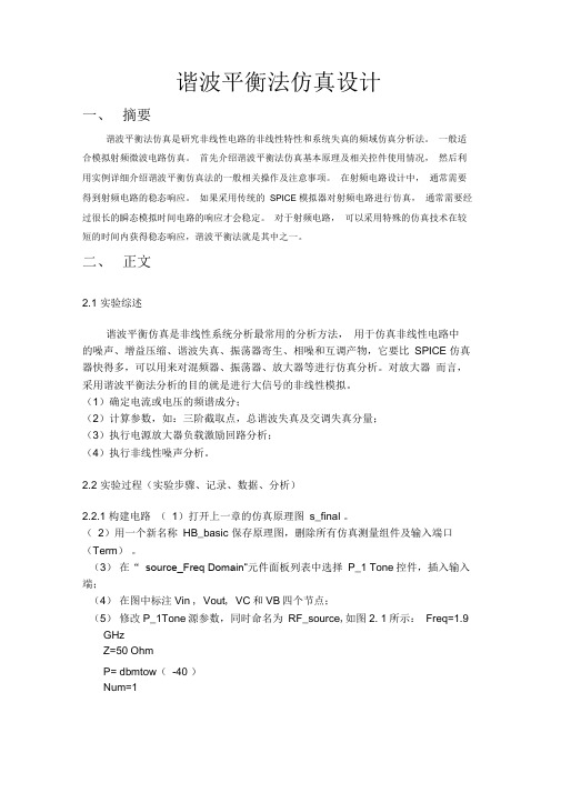
第8章 ADS系统级仿真 193║图8.12 添加20dB时的Plot Trace & Attributes窗口图8.13 放大器增益为10dB和20dB时的S21曲线8.1.3 原理图谐波平衡仿真在对原理图进行谐波平衡仿真之前,需要对原理图进行修改。
下面将修改原理图,并对修改后的原理图进行谐波平衡仿真。
1.修改原理图(1)另存原理图在原理图RF_system1上,选择菜单【File】→【Save Design As】,弹出【Save Design As】对话框,在【Save Design As】对话框中,输入文件名RF_system2,然后单击“保存”,将原理图另存为RF_system2。
(2)删除元器件在原理图RF_system2上修改原理图,修改时首先删除一些元器件,删除的元器件如下。
终端负载Term1。
V_1Tone单频电压源、50Ω电阻。
S参数仿真控制器。
(3)设置单频功率源在原理图中选择频域源【Sources-Freq Domain】元器件面板,在电路的输入端插入单频功率源P_1Tone,对单频功率源P_1Tone设置如下。
P =polar(dbmtow(−40),0),表示单频功率源输出信号的功率为−40dBm。
Freq =1.9GHz,表示单频功率源的频率为1.9GHz。
(4)设置另一个单频功率源在原理图中选择频域源【Sources-Freq Domain】元器件面板,在电路的本振端插入单频功率源P_1Tone,对单频功率源P_1Tone设置如下。
P =polar(dbmtow(0),0),表示单频功率源输出信号的功率为0dBm。
Freq =1.8GHz,表示单频功率源的频率为1.8GHz。
(5)插入节点在原理图的输出端,插入节点V out。
应用ADS 设计混频器1. 概述图1为一微带平衡混频器,其功率混合电路采用3dB 分支线定向耦合器,在各端口匹配的条件下,1、2为隔离臂,1到3、4端口以及从2到3、4端口都是功率平分而相位差90°。
图1设射频信号和本振分别从隔离臂1、2端口加入时,初相位都是0°,考虑到传输相同的路径不影响相对相位关系。
通过定向耦合器,加到D1,D2上的信号和本振电压分别为: D1上电压 )2cos(1πω-=t V v s s s 1-1)cos(1πω-=t V v L L L 1-2D2上电压)cos(2t V v s s s ω= 1-3)2cos(2πω+=t V v L L L 1-4可见,信号和本振都分别以2π相位差分配到两只二极管上,故这类混频器称为2π型平衡混频器。
由一般混频电流的计算公式,并考虑到射频电压和本振电压的相位差,可以得到D1中混频电流为:∑∑∞-∞=∞-+-=m n L s m n t jn t jm I t i ,,1)]()2(exp[)(πωπω同样,D2式中的混频器的电流为:∑∑∞-∞=∞++=m n L s m n t jn t jm I t i ,,2)]2()(exp[)(πωω当1,1±=±=n m 时,利用1,11,1-++-=I I 的关系,可以求出中频电流为:]2)cos[(41,1πωω+-=+-t I i L s IF主要的技术指标有:1、噪音系数和等效相位噪音(单边带噪音系数、双边带噪音系数);2、变频增益,中频输出和射频输入的比较;3、动态范围,这是指混频器正常工作时的微波输入功率范围;4、双频三阶交调与线性度;5、工作频率;6、隔离度;7、本振功率与工作点。
设计目标:射频:3.6 GHz ,本振:3.8 GHz ,噪音:<15。
2.具体设计过程2.1创建一个新项目◇ 启动ADS◇ 选择Main windows◇ 菜单-File -New Project ,然后按照提示选择项目保存的路径和输入文件名 ◇ 点击“ok ”这样就创建了一个新项目。
实验一、ADS仿真基础内容一、电路仿真基础实验目的:1、熟悉ADS的基础界面;2、掌握ADS文件的基本操作;3、依照示例完成简单电路的设计仿真练习及调试;实验任务1、建立一个新的项目和原理图设计2、设置并执行S参数模拟3、显示模拟数据和储存4、在模拟过程中调整电路参数5、使用例子文件和节点名称6、执行一个谐波平衡模拟7、在数据显示区写一个等式实验步骤1.运行ADS在开始菜单中选择“Advanced Design System 2006A → Advanced Design System”(见图一)。
图一、开始菜单中ADS 2006A的选项用鼠标点击后出现初始化界面。
随后,很快出现ADS主菜单。
图三、ADS主菜单如果,你是第一次打开ADS,在打开主菜单之前还会出现下面的对话框。
询问使用者希望做什么。
图四、询问询问使用者希望做什么的对话框其中有创建新项目(Create a new project);打开一个已经存在的项目(Open a existing project);打开最近创建的项目(Open a recently used project)和打开例子项目(Open an example project)四个选项。
你可以根据需要打开始当的选项。
同样,在主菜单中也有相同功能的选项。
如果,你在下次打开主菜单之前不出现该对话框,你可以在“Don’t display this dialog box again”选项前面的方框内打勾。
2.建立新项目a.在主窗口,通过点击下拉菜单“File→New Project…”创建新项目。
图五、创建新项目对话框其中,项目的名称的安装目录为ADS项目缺省目录对应的文件夹。
(一般安装时缺省目录是C:\user\default,你可以修改,但是注意不能用中文名称或放到中文名称的目录中,因为那样在模拟时会引起错误)。
在项目名称栏输入项目名称“lab1”。
对话框下面的项目技术文件主要用于设定单位。
《通信电子电路—ADS仿真》实验报告专业:班级:姓名:学号:教师:时间:实验项目实验一电路模拟基础 (02)实验二直流仿真和建立电路模型 (11)实验三交流(AC)仿真 (19)实验四 S参数仿真与优化 (26)实验五电路包络仿真 (36)Agilent公司推出的ADS软件以其强大的功能成为现今国内各大学和研究所使用最多的软件之一。
ADS电子设计自动化(EDA软件全称为Advanced Design System)是美国安捷伦(Agilent)公司所生产拥有的电子设计自动化软件;ADS功能十分强大,包含时域电路仿真(SPICE-like Simulation)、频域电路仿真(Harmonic Balance Linear Analysis)、三位电磁仿真(EM Simulation)、通信系统仿真(Communication System Simulation)和数字信号处理仿真软件(DSP);支持射频和系统设计工程师开发所有类型的RF设计,从简单到复杂,从离散的射频/微波模块到用于通信和航天/国防的集成MMIC,是当今国内各大学和研究所使用最多的微波/射频电路和通信系统仿真软件。
在本次实验中采用的软件版本为ADS2006。
实验一电路模拟基础一、概述本实验包括用户基础界面,ADS文件的创建过程包括建立原理图、仿真控件、仿真、和数据显示等部分的内容。
该实验还包括调谐与谐波平衡法仿真的一个简单例子。
二、任务1.建立一个新的项目和原理图设计2.设置并执行S参数模拟3.显示模拟数据和储存4.在模拟过程中调整电路参数5.使用例子文件和节点名称6.执行一个谐波平衡模拟7.在数据显示区写一个等式三、低通滤波器设计1.运行ADS2.建立新项目3.检查你的新项目内的文件4.建立一个低通滤波器设计5.设置S参数模拟6.开始模拟并显示数据7.储存数据窗口8.调整滤波器电路四、由行为模型构成的RF接收系统设计1.建立一个新的系统项目和原理图使用上一章学到的方法,建立一个新的项目取名rf_sys。
Harmonic Balance Simulation on ADSGeneral Description of Harmonic Balance in Agilent ADS 1Harmonic balance is a frequency-domain analysis technique for simulating nonlinear circuits and systems. It is well-suited for simulating analog RF and microwave circuits, since these are most naturally handled in the frequency domain. Circuits that are best analyzed using HB under large signal conditions are:power amplifiersfrequency multipliersmixersoscillatorsmodulatorsHarmonic Balance Simulation calculates the magnitude and phase of voltages or currents in a potentially nonlinear circuit. Use this technique to:Compute quantities such as P1dB, third-order intercept (TOI) points, total harmonic distortion (THD), and intermodulation distortion components Perform power amplifier load-pull contour analysesPerform nonlinear noise analysisSimulate oscillator harmonics, phase noise, and amplitude limitsIn contrast, S-parameter or AC simulation modes do not provide any information on nonlinearities of circuits. Transient analysis, in the case where there are harmonics and or closely-spaced frequencies, is very time and memory consuming since the minimum time step must be compatible with the highest frequency present while the simulation must be run for long enough to observe one full period of the lowest frequency present. Harmonic balance simulation makes possible the simulation of circuits with multiple input frequencies. This includes intermodulation frequencies, harmonics, and frequency conversion between harmonics. Not only can the circuit itself produce harmonics, but each signal source (stimulus) can also produce harmonics or small-signal sidebands. The stimulus can consist of up to twelve nonharmonically related sources. The total number of frequencies in the system is limited only by such practical considerations as memory, swap space, and simulation speed.The Simulation Process 1 (FYI – skip to next section if you want to get started now)The harmonic balance method is iterative. It is based on the assumption that for a given sinusoidal excitation there exists a steady-state solution that can be approximated to satisfactory accuracy by means of a finite Fourier series. Consequently, the circuit node 1 From Agilent ADS Circuit Simulation Manual, Chap. 7, Harmonic Balance.voltages take on a set of amplitudes and phases for all frequency components. The currents flowing from nodes into linear elements, including all distributed elements, are calculated by means of a straightforward frequency-domain linear analysis. Currents from nodes into nonlinear elements are calculated in the time-domain. Generalized Fourier analysis is used to transform from the time-domain to the frequency-domain.A frequency-domain representation of all currents flowing away from all nodes is available. According to Kirchoff's Current Law (KCL), these currents should sum to zero at all nodes. The probability of obtaining this result on the first iteration is extremely small.Therefore, an error function is formulated by calculating the sum of currents at all nodes. This error function is a measure of the amount by which KCL is violated and is used to adjust the voltage amplitudes and phases. If the method converges (that is, if the error function is driven to a given small value), then the resulting voltage amplitudes and phases approximate the steady-state solution.•Designers are usually most interested in a system's steady-state behavior. Many high-frequency circuits contain long time constants that require conventionaltransient methods to integrate over many periods of the lowest-frequency sinusoid to reach steady state. Harmonic balance, on the other hand, captures the steady-state spectral response directly.•The applied voltage sources are typically multitone sinusoids that may have very narrowly or very widely spaced frequencies. It is not uncommon for the highestfrequency present in the response to be many orders of magnitude greater than the lowest frequency. Transient analysis would require an integration over anenormous number of periods of the highest-frequency sinusoid. The time involved in carrying out the integration is prohibitive in many practical cases.•At high frequencies, many linear models are best represented in the frequency domain. Simulating such elements in the time domain by means of convolutioncan results in problems related to accuracy, causality, or stability.Harmonic Balance SetupThe HB method depends on calculating currents and voltages at many harmonically related frequencies for each fundamental signal under consideration. Since we are interested in the steady state solution of a nonlinear problem, we must allow the HB simulator to use enough harmonics so that a Fourier series constructed from these harmonic amplitudes and phases can reproduce a reasonable replica of the time domain solution.Figure 1 illustrates a very basic HB simulation setup. The Harmonic Balance controller specifies several key simulation parameters. In the example below, one fundamental frequency, Freq[1]=450 MHz, is specified as an input. The index [1] shows that only one fundamental frequency is being considered. Order[1] specifies the number of harmonic frequencies to be calculated (15) for the first (and only) frequency in this case. One of the most common errors in HB simulation setup is to use too low of an order. You candetermine what order is optimum if you first simulate your circuit with a small order then increase the order in steps of 1 or 2 harmonics. When the solution stops changing within a significant bound, you have reached the optimum order. Using too high of an order is wasteful of memory, file size and simulation time, so it is not efficient to just clobber the problem with a very high order. Some user discretion is advised.Figure 1. Example of the HB controller used for a very simple single tone (frequency) simulation. In addition, power PIN is being swept from -10 to 6 dBm.ADS does not automatically pass parameters from the schematic to the display panel. Calculated node voltages are automatically transferred, but the input parameters used for independent voltage, current or power sources are not (unless they are being swept by a sweep controller setting. Then they become a parameter that is automatically passed to the display.). To transfer parameters from schematic to display, open the controller symbol, select output tab, and then add the variables to the list as seen below:The fundamental frequency of the input source must be the same as specified on the controller. The Sources-Freq Domain palette includes many sources suitable for use with HB. The single tone source P_1Tone is illustrated below. This source provides a single frequency sinusoid at a specified available power. Here we see that the internal source resistance (50 ohms) is included. The available source power is provided as PIN (indBm, which will be converted to Watts by the dbmtow function) and degrees of phase.must be specified.You could also have selected a voltage source, V_1Tone, or for multiple frequency simulations, there are V_nTone and P_nTone sources. These are often used for intermodulation distortion simulations. Voltage or current sources require an external source resistance or impedance whereas the power sources include an internal source resistance or impedance, Z.Nodes must be labeled in the harmonic balance simulation in order to transfer their voltages to the display. If currents are to be used in calculations as well, a current probe must be inserted from the Probe Components menu. An example of a PA output network is shown in the next figure. Nodes Vce and Vload are labeled using the Insert pulldown menu: Insert > Wire/Pin Label. This opens a text box where you can enter the node name you want. I_ce and I_load were measured with the current probes as shown.Figure 3. PA output circuit showing node voltage and current labels and probes. Displaying resultsThe output voltages and currents calculated by the HB analysis will contain many frequency components. You can display all of them in a spectral display by just plotting the voltage or current on an X-Y plot. Markers can be used to read out the spectral line amplitudes or powers.Figure 4. Spectrum in dBm is plotted for Vload. You can see the 15 harmonics.Often you will want to plot power in dBm. If your load impedance is real, you can use the dbm function in an equation. If the load has a complex impedance, then use the definition for sinusoidal power.30)))._(*(*5.0log(*10_+=i load I conj Vload real P dBm outThis will give you the power in dBm in all cases. This is the preferred method. Note that calculated quantities much below – 100 dBm are probably not very reliable due to the limited precision of the device modelsTo perform calculations of power and efficiency, you will want to be able to selectspecific frequency components. The harmonic index (harmindex) can be used to do this. If you plot your output variable in a table format, you will see a list of frequencies.Figure 5. Table showing the value of Pout and Pout_dBm at several harmonicfrequencies. The frequencies are printed in order and can be designated by an index, ranging from 0 for DC to Order – 1 for the highest harmonic frequency.The first frequency in the table is DC and has index 0. Fundamental is index 1. So, to select the voltage at the fundamental frequency, for example, you could write Vload[1] or to select power, Pout[1] or Pout_dBm[1] in this example. The second harmonic would bePout[2]. Of course, we do not need to draw a table to use the index. For example, the DC component of the power supply voltage can be extracted by using the 0 index: VCC[0]. Then, if the supply voltage and current were measured and passed to the output display, you could calculate DC input power byTo display the results of equations such as this, you use the table or rectangular plot features in the display panel. The data set must be changed to Equations as shown in order to find the result of the calculations.Figure 6. To plot the results of an equation in the data display, select Equations in the data setIf you want to see the time domain version of a voltage or current, the display can perform the inverse Fourier transform while plotting. Select the Time domain signal option.Figure 7. When plotting HB data, you must convert it to a scalar quantity (dB, dBm, or magnitude). Notice that a time domain conversion can also be performed by an FFT if requested.Figure 8. Example of a time domain plot from a HB simulation.Once the simulation has been run, the data is available on the display panel. You can use equations to calculate power, gain, and power added efficiency. Note the use of theindices once again.Parameter SweepsIt is possible to sweep any of the independent parameters in the HB simulation. To set upthe sweep, double click on the Harmonic Balance Controller.Figure 9. Selecting the Sweep tab allows you to sweep one independent variable.Click on the Sweep tab. Choose the parameter to be swept, the sweep type (Linear, Log), and the Start, Stop, and Step variables (or number of points instead of step-size). In this example, we are sweeping the input power to the amplifier to determine the gain compression behavior. The more sweep points chosen, the longer the simulation time and the greater the data file size.2Figure 10. A double axis plot of Pout vs Pin and PAE vs. Pin for a power amplifier.2 If two variables are to be swept, a ParamSweep controller icon from the HB menu must be added to the schematic.Figure 11. Amplifier gain vs. Pin.From this plot, we can see that the P1dB compression input power is about 4 dBm.Multiple frequency simulationsMultiple frequencies or “tones” (mainly two-tone) are widely used for evaluation of intermodulation distortion in amplifiers or mixers. In fig. 12, you can see that now two frequencies have been selected, Freq[1] and Freq[2]. Each frequency must also declarean order (number of harmonic frequencies to be considered).Figure 12. HB controller example for a two-tone PA simulation.Intermodulation distortion occurs when more than one input frequency is present in the circuit under evaluation. Therefore, additional frequencies need to be specified when setting up for this type of simulation. Two-tone simulations are generally performed with two closely spaced input frequencies. In this example, the two inputs are at 449.8 and 450.2 MHz. The frequency spacing must be small enough that the two tones are well within the signal bandwidth of the circuit under test.Maximum order corresponds to the highest order mixing product (n + m) to be considered (n*freq[1] ± m*freq[2]). There will be a frequency component in the output file corresponding to all possible combinations of n and m up to the MaxOrder limit. The simulation will run faster with lower MaxOrder and fewer harmonics of the sources, but may be less accurate. Often accurate IMD simulations will require a large maximum order. In this case, a larger number of spectral products will be summed to estimate the time domain waveform and therefore provide greater accuracy. This will increase the size of the data file and time required for the simulation. Increase the orders and MaxOrder in increments of 2 and watch for changes in the IMD output power. When no further significant change is observed, then the order is large enough. If large asymmetry is noted in the intermodulation components, higher orders are indicated..Sometimes, increasing the oversampling ratio for the FFT calculation (use the Param menu of the HB controller panel) can reduce errors. This oversampling controls the number of time points taken when converting back from time to frequency domain in the harmonic balance simulation algorithm. A larger number of time samples increases the accuracy of the tranform calculation but increases memory requirements and simulation time. Both order and oversampling should be increased until you are convinced that further increases are not worthwhile.For multiple frequency simulations, the simulation time will be reduced substantially by using the Krylov option which can be selected on the Display tab of the HB controller. The two tone source frequencies are provided with a P_nTone generator from the Sources – Freq Domain menu. The two frequencies are sometimes specified in a Var block. The same approach is used to specify frequencies in the HB controller so that the effect caused by changes in deltaF could be evaluated by changing only one variable. The available power, PIN, is specified in dBm for each source frequency.Figure 13. Two-tone source example.Displaying Results of Multitone SimulationsYou can view the result around the fundamental frequencies by disabling the autoscale function in the plot and specifying your own narrow range. The display below shows intermodulation products up to the 7th order (MaxOrder specified on the HB controller).Fig. 14.We would like to study the output voltage at the fundamental frequencies and the third-order IMD product frequencies. This can be selected from the many frequencies in the output data set by using the mix function. The desired frequencies could be selected by: (RFfreq + deltaF) V fund1 = mix(Vload,{1,0}).(RFfreq - deltaF) V fund2 = mix(Vload,{0,1})(2*(RFfreq +deltaF)-RFfreq - deltaF) V IM1 = mix(Vload,{2,-1})(2*(RFfreq - deltaF)-RFfreq + deltaF) V IM2 = mix(Vload,{-1,2})The respective indices used with the mix function to select this frequency are shown to the right. The indices in the curly brackets are ordered according to the HB fundamental analysis frequencies.Mixer SimulationsIn the case of a mixer simulation, at least 2 frequencies are always needed: LO and RF. Figure 16 shows an example of the setup used for a two-tone simulation of a mixer. The format is similar to that described above for power amplifier two tone simulations except now 3 frequencies are required. The frequency with the highest power level (in thisexample, the LO) is always the first frequency to be designated in the harmonic balance controller. Other inputs follow sequencing from highest to lowest power.Figure 16. HB controller example for a mixer simulation.The harmonic order should be higher for high amplitude signals. For the example above, the LO order is highest because it is intended to switch the mixer. The RF orders can be smaller since they are rarely of high amplitude compared with the LO.In the case of a mixer simulation, we would like to study the output voltage at the IF frequency. This must be selected from many frequencies in the output data set. A particular frequency is selected by using the mix function. In this example, the desired IF frequencies could be:LOfreq – (RFfreq + Fspacing/2) V IF = mix(Vout,{1,-1,0}).LOfreq – (RFfreq - Fspacing/2) V IF = mix(Vout,{1,0,-1})LOfreq + (RFfreq + Fspacing/2) V IF = mix(Vout,{1,1,0})LOfreq + (RFfreq - Fspacing/2) V IF = mix(Vout,{1,0,1})and the respective indices used with the mix function to select this frequency are shown to the right. The indices in the curly brackets are ordered according to the HB fundamental analysis frequencies. Thus, {1,-1,0} selects 1*LOfreq – 1*RFfreq[1]+0*RFfreq[2].DesignGuidesThere are so many types of simulations that could be performed on a mixer that it is not reasonable to try to describe them all in this tutorial. Instead, you can use the Mixer DesignGuide, a set of schematic and display templates that can be pulled into your project file. Go to the DesignGuides pulldown menu and select Mixer DesignGuide. Choose a representative sample mixer schematic to modify if you want to create your own mixer circuit. Determine whether your mixer is single ended or differential. The differential circuit templates include baluns; single-ended do not. Choose from a large set of simulation types, some with parameter sweeps, some without.Refer to the Mixer Design Guide tutorial for more information.Convergence WoesAny user of the harmonic balance simulator will eventually encounter convergence problems. Unfortunately, when this happens, no useful information is provided by the simulator. Problems with convergence generally arise when the circuit under simulation is or becomes highly nonlinear. In the case of mixers, there are inherent nonlinearities that are required for the mixing process, but these are usually not so bad unless you are seriously overdriving one of the inputs. If the simulation fails, check the biasing of the transistors. HB doesn’t do well with BJTs driven into their saturation region. If that is not the problem, then try decreasing either LO power or the RF power sweep range. You may be driving the mixer well beyond saturation when using default power levels in mixer DG templates. As a last resort, you can try using the Direct solver rather than Krylov, but this will increase simulation time by a large factor.。