Matlab第十章作业

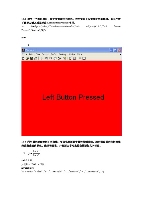
10-2建立一个图形窗口，使之背景颜色为红色，并在窗口上保留原有的菜单项，而且在按下鼠标左键之后显示出Left Button Pressed 字样。

>> hf=figure('color','r','windowbuttondownfcn','axis off;text(0.1,0.5,''Left Button Pressed'',''fontsize'',30)')hf =110-3利用图形对象绘制下列曲线，要求先利用缺省属性绘制曲线，然后通过图形句柄操作来改变曲线的颜色、线型和线宽，并利用文字对象给曲线添加文字标注。

（1）4211x x y ++= x=0:0.1:10;y=((1+x.^2)/(1+x.^4));hf=plot(x,y);>> set(hf,'color','r','linestyle',':','marker','*','linewidth',1);（4）⎪⎩⎪⎨⎧==325ty t x >> t=0:2:100;>> x=t.*t;>> y=5*t.^3;>> hf=plot(x,y);>>set(hf,'color','b','linestyle',':','marker','p','linewidth',0.3);10-4利用图形对象绘制下列三维图形，要求与上题相同。

（1）⎪⎩⎪⎨⎧===t z t y t x sin cos>> t=0:0.1:2*pi;>> x=cos(t);>> y=sin(t);>> z=t;>> hf=plot3(x,y,z);z（4）3y>> x=0:1:50;>> y=0:1:50;>> z=y.^3;>> hf=plot3(x,y,z);。

MATLAB作业⼀、必答题：1. MATLAB系统由那些部分组成？答：MATLAB系统主要由开发环境、MATLAB语⾔、MATLAB数学函数库、图形功能和应⽤程序接⼝五个部分组成。

2. 如何启动M⽂件编辑/调试器？答：在操作界⾯上选择“建⽴新⽂件”或“打开⽂件”操作时，M⽂件编辑/调试器将被启动。

在命令窗⼝中键⼊“edit”命令也可以启动M⽂件编辑/调试器。

3. 存储在⼯作空间中的数组能编辑吗？如何操作？答：存储在⼯作空间的数组可以通过数组编辑器进⾏编辑：在⼯作空间浏览器中双击要编辑的数组名打开数组编辑器，再选中要修改的数据单元，输⼊修改内容即可。

4. 在MATLAB中有⼏种获得帮助的途径？答：在MATLAB中有多种获得帮助的途径：（1）帮助浏览器：选择view菜单中的Help菜单项或选择Help菜单中的MATLAB Help菜单项可以打开帮助浏览器；（2）help命令：在命令窗⼝键⼊“help” 命令可以列出帮助主题，键⼊“help 函数名”可以得到指定函数的在线帮助信息；（3）lookfor命令：在命令窗⼝键⼊“lookfor 关键词”可以搜索出⼀系列与给定关键词相关的命令和函数（4）模糊查询：输⼊命令的前⼏个字母，然后按Tab键，就可以列出所有以这⼏个字母开始的命令和函数。

5. 有⼏种建⽴矩阵的⽅法？各有什么优点？答：（1）以直接列出元素的形式输⼊；（2）通过语句和函数产⽣；（3）.在m⽂件中创建矩阵；（4）从外部的数据⽂件中装⼊。

6. 命令⽂件与函数⽂件的主要区别是什么？答：命令⽂件: M⽂件中最简单的⼀种，不需输出输⼊参数，⽤M ⽂件可以控制⼯作空间的所有数据。

运⾏过程中产⽣的变量都是全局变量。

运⾏⼀个命令⽂件等价于从命令窗⼝中顺序运⾏⽂件⾥的命令，程序不需要预先定义，只要依次将命令编辑在命令⽂件中即可。

函数⽂件：如果M⽂件的第⼀个可执⾏⾏以function开始，便是函数⽂件，每⼀个函数⽂件定义⼀个函数。

第十章Matlab软件简介1984年，MathWorks公司把内核采用C语言编写的Matlab正式推向市场，Matlab的名称由Matrix(矩阵)和Laboratory(实验室)两词的前三个字母组合而成。

Matlab集数值分析、矩阵运算、符号运算及图形处理等强大功能于一体，且包含一系列规模庞大、覆盖不同领域的工具箱(Toolbox)，再加上它简单易学、实用方便，从问世之初，就深受广大科技工作者的欢迎，现已成为许多学科领域中计算机辅助设计与分析、算法研究和应用开发的基本工具和首选平台。

在发达国家的理工科院校，Matlab已经成为一门必修课程，国内的许多高校也陆续开设有关Matlab的课程。

我们在这里简单介绍一下Matlab的一些基本功能，为学生深入学习Matlab奠定基础，并最终希望学生能从繁重的编程劳动中脱离出来，把主要精力放在建立数学模型的环节上。

§10.1 基本操作Matlab软件安装好之后，双击系统桌面的Matlab图标，或在开始菜单的程序选项中选择Matlab快捷方式，即开始启动Matlab。

初次启动Matlab后，将进入Matlab默认设置的桌面平台。

桌面平台包括主窗口、命令窗口、历史窗口、当前目录窗口和工作间管理窗口等窗口，我们这里主要介绍命令窗口和主窗口的一些较为简单的功能。

工作空间窗口命令窗口历史窗口Matlab命令窗口如上图所示，其中“>>”为运算提示符，表示Matlab正处在准备状态，等待操作者在此提示符右侧输入运算命令。

例如我们想计算[(1+2)X3—4)]÷2^3]，只需在提示符“>>”后输入“((1+2)* 3-4)／2^3”，然后按Enter键(为书写方便，本章中的所有命令语句均用提示符“>>”开头，之后的按Enter键的动作用“↙”来表示)，命令窗口马上就会出现算式的结果0．625 0(如图10—2)，并出现新的提示符等待新的运算命令的输入。

中南大学matlab课后习题（10）Unit 1实验内容1.答：用help命令可以查询到自己的工作目录。

输入help命令：help <函数名>2.答：MATLAB的主要优点：通过例1-1至例1-4的验证，MATLAB的优点是MATLAB以矩阵作为数据操作的基本单位，使得矩阵运算变得非常简捷，方便，高效。

还提供了丰富的数值计算函数。

MATLAB绘图十分方便，只需输入绘图命令，MATLAB便可自动绘出图形。

3.答：INV(X) is the inverse of the square matrix X。

A warning message is printed if X is badly scaled or nearly singular. PLOT(X,Y) plots vector Y versus vector X. If X or Y is a matrix, then the vector is plotted versus the rows or columns of the matrix, whichever line up. If X is a scalar and Y is a vector, length(Y) disconnected points are plotted. PLOT(Y) plots the columns of Y versus their index. If Y is complex, PLOT(Y) is equivalent to PLOT(real(Y),imag(Y)).In all other uses of PLOT, the imaginary part is ignored. For vectors, MAX(X) is the largest element in X. For matrices,MAX(X) is a row vector containing the maximum element from each column. For N-D arrays, MAX(X) operates along the first non-singleton dimension. [Y,I] = MAX(X) returns the indices of the maximum values in vector I. If the values along the first non-singleton dimension contain more than one maximal element, the index of the first one is returned. ROUND(X) rounds the elements of X to the nearest integers. MAX(X,Y) returns an array the same size as X and Y with the largest elements taken from X or Y. Either one can be a scalar。

西南科技大学本科生课程备课教案计算机技术在安全工程中的应用——Matlab入门及应用授课教师：徐中慧班级：专业：安全技术及工程第十章 MATLAB自定义函数课型：新授课教具：多媒体教学设备，matlab教学软件一、目标与要求✧通过解说与实例练习，掌握matlab创建函数M文件的方法✧掌握matlab中全局变量与局部变量的定义与用法✧通过解说与实例练习，掌握在matlab主函数M文件中创建子函数✧在实例练习过程中，回顾利用伪码编写简单程序的方法✧掌握通过创建matlab函数M文件解决生活中的计算问题二、教学重点与难点本堂课教学的重点在于引导学生掌握matlab中函数M文件的创建及应用。

本堂课的难点在于理解matlab中函数M文件主函数与子函数的区别及调用，局部变量与全局变量的定义与应用范围的区别。

三、教学方法本课程主要通过讲授法、演示法、练习法等相结合的方法来引导学生掌控本堂课的学习内容。

1)通过讲授法向学生讲述创建matlab函数M文件的基本方法、全局变量与局部变量的定义及用法等。

2)通过运用多媒体设备现场演示matlab创建函数M文件的应用实例。

3)在掌握创建matlab函数M文件基本方法的基础上，采用练习法引导学生创建函数M文件解决实际问题。

四、教学内容课后习题五（1）拉力测试装置在测试过程中，被测样本受均匀外力的作用产生形变。

下图中显示的是一组拉力测试数据。

根据以下公式计算应力与形变：00l l F A l σε-=和＝ 其中，σ是产生的应力，单位为lbf/in 2(psi);F 为施加的外力，单位为lbf;A 为样本的截面积，单位为in 2；ε为产生的形变，单位为in/in ；l 为样本的长度；0l 为样本的原始长度。

（a ）测试样本是直径为0.505in 的金属杆，根据直径可以计算出金属杆的截面积，进一步利用所提供的数据计算金属杆的应力和形变。

（b ）以形变为x 轴，应力为y 轴，作x-y 线图。

MATLAB 作业MATLAB Excise For Chapter2M2.2、1、程序：function d=M2_2(N)n=-N:N;x1=sin(0.8*pi*n+0.8*pi);x2=5*cos(1.5*pi*n+0.75*pi)+4*cos(0.6*pi*n)-sin(0.5*pi*n);subplot(2,1,1)stem(n,x1,'filled');grid onxlabel('TIME index :n');ylabel('2.30(b)');subplot(2,1,2)stem(n,x2,'filled');grid onxlabel('TIME index :n');ylabel('2.30(e)');2、调用并运行：M2_2（10）M2.3、1、程序：function s=M2_3(A,omega,fai,N)n=0:N;x=A*sin(omega*n+fai);stem(n,x,'fill');grid onaxis([0,N,-2,2]);xlabel('Time index n');ylabel('Amplitude');2、调用并运行(a)、M2_3(1.5,0,pi/2,40)、M2_3(1.5,0.1*pi,pi/2,40)、M2_3(1.5,0.2*pi,pi/2,40)、M2_3(1.5,0.8*pi,pi/2,40)、M2_3(1.5,0.9*pi,pi/2,40)、M2_3(1.5,pi,pi/2,40)、M2_3(1.5,1.1*pi,pi/2,40)、M2_3(1.5,1.2*pi,pi/2,40)(b)、（1）omega=0.6*pi周期T=10；理论上：T=10 （2）omega=0.28*pi周期T=50；；理论上：T=50；（3）omega=0.45*pi周期T=40；理论上：T=40；（4）omega=0.55*pi周期T=40；理论上：T=40；（4）omega=0.65*pi周期T=40；理论上：T=40；M2.9、MATLAB Excise For Chapter3M3.3、调用程序program 3-1运行M3_3Number of frequency points = [1000]Numerator coefficients = 0.2418*[1 0.139 -0.3519 0.139 1] Denominator coefficients = [1 0.2386 0.8258 0.1393 0.4153]The plot of the program are shown in below：运行M3_3Number of frequency points = [1000]Numerator coefficients = 0.1397*[1 -0.0911 0.0911 -1] Denominator coefficients = [1 1.1454 0.7275 0.1205]The plot of the program are shown in below：M3.7、h=input('Type in the target sequence= ');%输入要计算群延时的序列N=input('Type in the group delay frequency point=');%输入要计算的群延时点n=0:(length(h)-1);H=fft(h,N);K=fft(n.*h,N);tao=real(K./H)运行M3-7M3_7Type in the target sequence= [1 1 2 0 0 6 3]Type in the group delay frequency point=8tao =4.0769 7.7221 4.6923 4.0556 9.0000 4.05564.6923 7.7221MATLAB Excise For Chapter5 M5.11、程序function d=M5_1(N)k1=-N:N;x1=ones(1,2*N+1);omega=0:pi/500:2*pi;X1=freqz(x1,1,omega);X1dft=fft(x1);n1=0:1:2*N;figure(1),plot(omega/pi,abs(X1),2*n1/(2*N+1),abs(X1dft),'ro') xlabel('\omega/\pi'),ylabel('Amplitude');k2=0:N;x2=ones(1,N+1);X2=freqz(x2,1,omega);X2dft=fft(x2);n2=0:1:N;figure(2),plot(omega/pi,abs(X2),2*n2/(N+1),abs(X2dft),'ro') xlabel('\omega/\pi'),ylabel('Amplitude');k3=k1;x3=1-(abs(k3)/N);X3=freqz(x3,1,omega);X3dft=fft(x3);n3=n1;figure(3),plot(omega/pi,abs(X3),2*n3/(2*N+1),abs(X3dft),'ro') xlabel('\omega/\pi'),ylabel('Amplitude');x4=N+1-abs(k3);X4=freqz(x4,1,omega);X4dft=fft(x4);figure(4),plot(omega/pi,abs(X4),2*n3/(2*N+1),abs(X4dft),'ro') xlabel('\omega/\pi'),ylabel('Amplitude');x5=cos(pi*k3/(2*N));X5=freqz(x5,1,omega);X5dft=fft(x5);figure(5),plot(omega/pi,abs(X5),2*n3/(2*N+1),abs(X5dft),'ro') xlabel('\omega/\pi'),ylabel('Amplitude');实现了problem3.19中5个序列的求DTFT和DFT2、调用程序运行结果M5_1（8）The red circles denote the DFT samples.当N=8时序列y1的DTFT和DFT采样当N=8时序列y2的DTFT和DFT采样当N=8时序列y3的DTFT和DFT采样当N=8时序列y4的DTFT和DFT采样当N=8时序列y5的DTFT和DFT采样M5.21、程序x=input('the sequence one to convolution;');y=input('the sequence two to convolution;');X=fft(x);Y=fft(y);S=X.*Y;s=ifft(S)2、调用程序M5_2the sequence one to convolution;[5,-2,2,0,4,3]the sequence two to convolution;[3,1,-2,2,4,4]s =10.0000 9.0000 16.0000 44.0000 36.0000 29.0000 M5_2M5_2the sequence one to convolution;[2-j,-1-j*3,4-j*3,1+j*2,3+j*2] the sequence two to convolution;[-3,2+j*4,-1+j*4,4+j*2,-3+j]s =11.0000 +25.0000i -9.0000 +48.0000i 3.0000 +17.0000i 29.0000 + 0.0000i -10.0000 +12.0000iProgram for （c）N=4;n=0:1:N;x=cos(pi*n/2);y=3.^n;X=fft(x);Y=fft(y);S=X.*Y;s=ifft(S)s =-23.0000 -69.0000 35.0000 105.0000 73.0000M5.81、程序X=[11 8-j*2 1-j*12 6+j*3 -3+j*2 2+j 15];k=8:12;XR(k)=conj(X(mod(-k+2,12)));XC=[X XR(k)];x=ifft(XC);n=0:1:11;x1=exp(i*2*pi*n/3);y=x1.*x;output=[x(1) x(7) sum(x) sum(y)];disp(output)disp(sum(x.*x))2、调用程序M5_84.5000 -0.8333 11.0000 -3.0000 - 2.0000i 74.8333MATLAB Excise For Chapter6M6.1(a)、The output of program6_1 by input the coefficient of problem （a）Numerator factors1.00000000000000 -2.10000000000000 5.000000000000001.00000000000000 -0.40000000000000 0.90000000000000Denominator factors1.000000000000002.00000000000000 4.999999999999991.00000000000000 -0.20000000000000 0.40000000000001Gain constant0.50000000000000Then ，The pole-zero plot of is given below:There are 3 ROCs associated with :R1,|z|<;R2,<|z|<; R3,|z|>The inverse –transform corresponding to the ROC is a left-sided sequence, the inverse–transform corresponding to the ROC is a two-sided sequence, and the inverse –transform corresponding to the ROC is a right-sided sequence.(b)、The output of program6_1 by input the coefficient of problem （b）Numerator factors1.00000000000000 1.20000000000000 3.999999999999991.00000000000000 -0.50000000000000 0.90000000000001Denominator factors1.000000000000002.10000000000000 4.000000000000011.00000000000000 0.60000000000003 01.00000000000000 0.39999999999997 0Gain constant1Then ，The pole-zero plot of is given below:There are 4 ROCs associated with :R1,|z|<R2,<|z|<; R3,<|z|<; R4,|z|>The inverse –transform corresponding to the ROC is a left-sided sequence, the inverse–transform corresponding to the ROC is a two-sided sequence, and the inverse –transform corresponding to the ROC is a right-sided sequence.M6.3The output of programme6_4 by type in：（a）M6_3Type in the residues = [-0.8,-7/6]Type in the poles = [-0.2,-1/6]Type in the constants = 3The output is as following：Numerator polynomial coefficients1.0333 0.7333 0.1000Denominator polynomial coefficients1.0000 0.3667 0.0333Hence（b）Rewrite X2（z）asM6_3Type in the residues = [3,-0.7+j*0.6454972243679,-0.7-j*0.6454972243679] Type in the poles = [-0.4,j*0.774596669,-j*0.774596669]Type in the constants = -2.5The output is as following：Numerator polynomial coefficients-0.9000 -2.5600 -0.1000 -0.6000Denominator polynomial coefficients1.0000 0.4000 0.6000 0.2400Hence，（c）M6_3Type in the residues = [5,1.5,-0.25]Type in the poles = [-0.64,-0.5,-0.5]Type in the constants = 0The output is as following：Numerator polynomial coefficients6.2500 6.5500 1.7300 0Denominator polynomial coefficients1.0000 1.6400 0.8900 0.1600Hence，（d）Rewrite X4（z）asM6_3Type in the residues = [-0.75,-0.375+j*0.2905,-0.375-j*0.2905] Type in the poles = [0.5,-j*0.4303,j*0.4303]Type in the constants = -5The output is as following：Numerator polynomial coefficients-4.5000 -6.8750 -3.6375 -0.8438Denominator polynomial coefficients1.0000 1.5000 0.7875 0.1688MATLAB Excise For Chapter7M7.31、程序k = input('Number of frequency points = ');num = input('Numerator coefficients = ');den = input('Denominator coefficients = ');w = 0:pi/(k-1):pi;h = freqz(num, den, w);plot (w,20*log10(abs(h)));gridxlabel('Normalized frequency'); ylabel('Gain, dB');2、调用M7_3运行结果如下M7_3Number of frequency points = 1000Numerator coefficients = [0,1,-2,1]Denominator coefficients = [1,-1.28,0.61+0.4*0.88,-(0.4*0.61)]From the gain response of the transfer function we can get that when the frequency become high and stable then we can conclude that this has a high pass responseM7.51、程序k = input('Number of frequency points = ');num = input('Numerator coefficients = ');den = input('Denominator coefficients = ');w = 0:pi/(k-1):pi;h = freqz(num, den, w);figure(1),plot(w/pi,abs(h));grid ontitle('Magnitude Spectrum')xlabel('\omega/\pi'); ylabel('Magnitude')figure(2),plot(w/pi,angle(h));grid ontitle('Phase Spectrum')xlabel('\omega/\pi'); ylabel('Phase, radians')2、调用M7_5运行结果如下M7_5Number of frequency points = 1000Numerator coefficients = 0.2031*[1,-(1+0.2743),1+0.2743,-1]Denominator coefficients =[1,0.487+0.1532,0.8351+0.83+0.1532*0.487+0.84,0.1532*0.84+0.487*0.8352,0.84*0.8351]Fro m the magnitude response plot given above it can be seen that represents a highpass filter. The difference equation representation of is given byy[n]+0.7074y[n-1]+0.7976y[n-2]+0.2004y[n-3]=0.2031x[n]-0.2588x[n-1]+0.2588x[n-2]-0.2031x[n-3]MATLAB Excise For Chapter9M9.21、程序Fp = input('Passband edge frequency in Hz = ');Fs = input('Stopband edge frequency in Hz = ');FT = input('Sampling frequency in Hz = ');Rp = input('Passband ripple in dB = ');Rs = input('Stopband minimum attenuation in dB = ');Wp = 2*Fp/FTWs = 2*Fs/FT[N, Wn] = buttord(Wp, Ws, Rp, Rs)[b, a] = butter(N, Wn);disp('Numerator polynomial');disp(b)disp('Denominator polynomial');disp(a)[h, w] = freqz(b, a, 512);figure（1），plot(w/pi, 20*log10(abs(h))); grid axis([0 1 -60 5]);xlabel('\omega/\pi'); ylabel('Magnitude, dB'); figure（2），plot(w/pi, unwrap(angle(h))); grid axis([0 1 -8 1]);xlabel('\omega/\pi'); ylabel('Phase, radians');2、调用M9_2运行结果如下M9_2Passband edge frequency in Hz = 10000Stopband edge frequency in Hz = 30000Sampling frequency in Hz = 100000Passband ripple in dB = 0.4Stopband minimum attenuation in dB = 50Wp =0.2000Ws =0.6000N =5Wn =0.2613Numerator polynomial0.0039 0.0197 0.0394 0.0394 0.0197 0.0039Denominator polynomial1.0000 -2.3611 2.6131 -1.5486 0.4864-0.0636M9.111、（a）TF=9kHZ，1pF=1.2kHZ，2pF=2.2kHZ，1sF=650HZ，2sF=3kHZ pα=0.8dB，sα=31dBThenTpp FF112πω==0.8378，Tpp FF222πω==1.536，Tss FF112πω==0.4538，Tss FF222πω==2.094According to bilinear transformation method ：)2tan(11ppω=ΩΛ=0.445，)2tan(22ppω=ΩΛ=0.996，)2tan(11ssω=ΩΛ=0.231，)2tan(22s s ω=ΩΛ=1.731. ωB =2p ΛΩ—1p ΛΩ=0.521，s Ω=3.13程序[N, Wn] = cheb1ord(1, 3.13, 0.8, 31, 's');[B, A] = cheby1(N, 0.8, Wn, 's');[BT, AT] = lp2bp(B, A, sqrt(0.43), 0.521);[num, den] = bilinear(BT, AT, 0.5);[h, omega] = freqz(num, den, 256);plot(omega/pi, 20*log10(abs(h)));grid;xlabel('\omega/\pi'); ylabel('Gain,in dB');title('Chebyshev I Bandpass Filter');axis([0 1 -60 5]);2、调用M9_11运行结果如下MATLAB Excise For Chapter10M10.11、程序M1= input('M1= ');M2= input('M2= ');n1=-M1:0.5:M1;n2=-M2:0.5:M2;num1=-0.4*sinc(0.4*n1);num2=-0.4*sinc(0.4*n2);num1(M1+1)=0.6;num2(M2+1)=0.6;w1= 0:pi/(4*M1):pi;w2= 0:pi/(4*M2):pi;h1= freqz(num1, 1, w1);h2= freqz(num2, 1, w2);plot(w1/pi,abs(h1),w2/pi,abs(h2));grid ontitle('Magnitude Spectrum')xlabel('\omega/\pi'); ylabel('Magnitude')2、调用程序运行结果M10.51、程序N = 36;fc = 0.2*pi;M = N/2;n = -M:1:M;t = fc*n;lp = fc*sinc(t);b = 2*[lp(1:M) (lp(M+1) - 0.5) lp((M+2):N+1)]; bw = b.*hamming(N+1)';[h2, w] = freqz(bw, 1, 512);plot(w/pi, abs(h2));axis([0 1 0 1.2]);xlabel('\omega/\pi');ylabel('Magnitude');title(['\omega_c = ', num2str(fc), ', N = ', num2str(N)]);grid on 2、运行结果M10.81、程序wp = 4*(2*pi)/18;ws = 6*(2*pi)/18;wc = (wp + ws)/2;dw = ws - wp;% HammingM = ceil(3.32*pi/dw);N = 2*M+1;n = -M:M;num = (6/18)*sinc(6*n/18);wh = hamming(N)';b = num.*wh;figure(1);k=0:2*M;stem(k,b);title('Impulse Response Coefficients');xlabel('Time index n'); ylabel('Amplitude');figure(2);[h, w] = freqz(b,1,512);plot(w/pi, 20*log10(abs(h))); grid;xlabel('\omega/\pi'); ylabel('Gain, in dB');title('Lowpass filter designed using Hamming window');axis([0 1 -80 10]);% HannM = ceil(3.11*pi/dw);N = 2*M+1;n = -M:M;num = (6/18)*sinc(6*n/18);wh = hann(N)';b = num.*wh;figure(3);k=0:2*M;stem(k,b);title('Impulse Response Coefficients');xlabel('Time index n'); ylabel('Amplitude');figure(4);[h, w] = freqz(b,1,512);plot(w/pi, 20*log10(abs(h)));grid;xlabel('\omega/\pi');ylabel('Gain, in dB');title('Lowpass filter designed using Hann window'); axis([0 1 -80 10]);% BlackmanM = ceil(5.56*pi/dw);N = 2*M+1;n = -M:M;num = (6/18)*sinc(6*n/18);wh = blackman(N)';b = num.*wh;figure(5);k=0:2*M;stem(k,b);title('Impulse Response Coefficients');xlabel('Time index n'); ylabel('Amplitude');figure(6);[h, w] = freqz(b,1,512);plot(w/pi, 20*log10(abs(h)));grid;xlabel('\omega/\pi');ylabel('Gain, in dB');title('Lowpass filter designed using Blackman window'); axis([0 1 -80 10]);2、运行结果M10.91、程序beta = 3.631;N = 44;n = -N/2:N/2;num = (6/18)*sinc(6*n/18);wh = kaiser(N+1,beta)';b = num.*wh;figure(1);stem(b);title('Impulse Response Coefficients');xlabel('Time index n');ylabel('Amplitude')figure(2);[h, w] = freqz(b,1,512);plot(w/pi, 20*log10(abs(h)));grid;xlabel('\omega/\pi');ylabel('Gain, in dB');title('Lowpass filter designed using Kaiser window'); axis([0 1 -80 10]);2、运行结果。

matlab教材习题答案Matlab是一种广泛应用于科学与工程领域的计算机编程语言和环境。

它具备强大的数值计算和数据可视化功能，被广泛用于数据分析、信号处理、图像处理、机器学习等领域。

对于初学者而言，掌握Matlab的基本语法和常用函数是非常重要的，而教材习题则是帮助学生巩固所学知识的重要资源。

本文将为大家提供一些Matlab教材习题的参考答案，以帮助读者更好地学习和应用Matlab。

1. 基本语法练习题1.1 计算并输出1到10的平方for i = 1:10fprintf('%d的平方是：%d\n', i, i^2);end1.2 计算并输出1到10的阶乘for i = 1:10fact = 1;for j = 1:ifact = fact * j;endfprintf('%d的阶乘是：%d\n', i, fact);end2. 数值计算练习题2.1 求解一元二次方程的根a = 1;b = -3;c = 2;delta = b^2 - 4*a*c;x1 = (-b + sqrt(delta))/(2*a);x2 = (-b - sqrt(delta))/(2*a);fprintf('一元二次方程的根为：%f, %f\n', x1, x2);2.2 求解线性方程组的解A = [1 2; 3 4];B = [5; 6];X = inv(A) * B;fprintf('线性方程组的解为：%f, %f\n', X(1), X(2));3. 数据处理练习题3.1 统计一个数组中的最大值、最小值和平均值data = [1, 2, 3, 4, 5];max_value = max(data);min_value = min(data);average_value = mean(data);fprintf('最大值：%f\n最小值：%f\n平均值：%f\n', max_value, min_value, average_value);3.2 对一个矩阵进行排序matrix = [4 2 3; 1 5 6; 9 8 7];sorted_matrix = sort(matrix);fprintf('排序后的矩阵为：\n');disp(sorted_matrix);4. 图像处理练习题4.1 读取并显示一张图片image = imread('image.jpg');imshow(image);4.2 对一张图片进行灰度化处理gray_image = rgb2gray(image);imshow(gray_image);5. 信号处理练习题5.1 生成并绘制正弦信号t = 0:0.01:2*pi;x = sin(t);plot(t, x);5.2 对一段音频信号进行傅里叶变换[y, fs] = audioread('audio.wav');Y = fft(y);plot(abs(Y));通过以上几个例子，我们可以看到Matlab的强大功能和灵活性。