Chapter_15 The Demand for Money多恩布什宏观经济学(教学课件)PPT
- 格式:ppt
- 大小:1.21 MB
- 文档页数:19
宏观经济学课件O.BlanchardMacro-economics6thchapter15Macroeconomics, 6e (Blanchard/Johnson)Chapter 15: Financial Markets and Expectations15.1 Multiple Choice Questions1) The length of time over which a bond promises to make payments to the holder is called which of the following?A) the term structure of interest ratesB) the face valueC) the yield to maturityD) the holding periodE) none of the aboveAnswer: EDiff: 12) A "junk bond" is a bond with aA) low yield to maturity.B) value of zero.C) low face value, but high coupon rate.D) high default risk.E) very low maturity.Answer: DDiff: 13) A bond has a face value of $10,000, a price of $12,000, and coupon payments of $2000 for two years. The coupon rate of this bond isA) 10%.B) 16.7%.C) 20%.D) 30%.E) none of the aboveAnswer: CDiff: 14) A discount bond is a bondA) with no coupon payments.B) where the price of the bond is greater than its face value.C) where the interest rate is zero.D) where the face value is zero.E) that never matures.Answer: ADiff: 15) For this question, assume that one-year and two-year bonds have the same risk; therefore, you can ignore risk here. Assuming that there is arbitrage between one-year bonds and two-year bonds, we know that the expected rate of return on two-year bondsA) will equal the expected rate of return from holding a one-year bond for one year.B) will equal the expected rate of return from holding a one-year bond for two years.C) will be larger than the expected rate of return from holding a one-year bond for one year.D) will be smaller than the expected rate of return from holding a one-year bond for one year.E) will be exactly half the rate of return on one-year bonds.Answer: ADiff: 26) A bond has a face value of $1,000, a price of $1,200, and coupon payments of $100 for two years. The "current yield" of this bond isA) 8.33%.B) 10%.C) 12%.D) 83%.E) none of the aboveAnswer: ADiff: 27) An upward-sloping yield curve suggests that financial market participants expect short-term interest rates willA) rise in the future.B) fall in the future.C) be unstable in the future.D) not change in the future.E) be equal to zero in the future.Answer: ADiff: 28) Suppose financial market participants expect short-term rates in the future to be less than current short-term interest rates. Given this information, we would expectA) an upward sloping yield curve.B) a downward sloping yield curve.C) an upward shifting yield curve.D) a downward shifting yield curve.E) a horizontal yield curve.Answer: BDiff: 29) Assume that the current one-year rate is 5% and the two-year rate is 7%. Given this information, the one-year rate expected one year from now isA) 5%.B) 6%C) 7%D) 9%E) 12%Answer: DDiff: 210) Suppose the current one-year interest rate is 4%, and financial markets expect the one-year interest rate next year to be 8%. Given this information, the yield to maturity on a two-year bond will be approximatelyA) 4%.B) 6%.C) 8%.D) 12%.E) none of the aboveAnswer: BDiff: 211) Suppose the current one-year interest rate is 4%. Also assume that financial markets expect the one-year interest rate next year to be 5%, and expect the one-year rate to be 6% the year after that. Given this information, the yield to maturity on a three-year bond will be approximatelyA) 4%.B) 5%.C) 6%.D) 15%.Answer: BDiff: 212) Which of the following bonds (of equal maturity) would have the largest risk premium?A) U.S. government bondsB) German government bondsC) the bonds of a financially stable corporation, like IBMD) Bondsbrated Aaa by Moody'sE) junk bondsAnswer: EDiff: 113) Suppose there is a decrease in the short-term interest rate. Give this reduction in the current short-term interest rate, which of the following will most likely occur?A) the long-term interest rate will increase.B) the long-term interest rate will remain the same.C) the long-term interest rate will decrease by more than the short-term rate.D) the long-term interest rate will decrease by the same amount as the short-term rate.E) the long-term interest rate will decrease, but by less than the short-term rate.Answer: EDiff: 214) Which of the following statements about indexed bonds is correct?A) they were relatively recently introduced in the United States.B) they exist in England.C) they have a nominal interest rate that rises when the inflation rate rises.D) all of the aboveE) none of the aboveAnswer: D15) Which of the following best explains why the long-term interest rate will generally change by less than 1% when the short-term interest rate changes by 1%?A) the mathematical calculations are more difficult for analysts in the case of long-term bonds.B) long-term rates are always lower than short-term rates, so there is less room for them to change.C) financial market participants will not expect this increase in the short-term interest rate to persist fully in the future.D) financial markets are often affected by bubbles and fads.E) none of the aboveAnswer: CDiff: 216) Equity finance is represented by which of the following?A) when a firm borrows money from banksB) when a firm sells bondsC) when a firm sells shares of stockD) when a firm draws down retained earningsE) when a firm sells off part of its capital stockAnswer: CDiff: 117) Among the following, which is the broadest measure of stock prices in the United States?A) Dow Jones IndexB) FT indexC) Nikkei IndexD) Term Structure IndexE) Standard and Poor's 500 Composite IndexAnswer: E18) The fundamental value of a share of stock is equal to which of the following?A) the sum of expected dividendsB) the present value of expected dividendsC) the sum of coupon paymentsD) the present value of coupon paymentsE) the present value of the expected yieldAnswer: BDiff: 119) A share of stock will pay a dividend of $25 in one year, and will be sold for an expected price of $500 at that time. If the current one-year interest rate is 5%, the current price of the stock will be approximately equal toA) $100.B) $475.C) $500.D) $525.E) none of the aboveAnswer: CDiff: 220) For this question, assume that there is perfect arbitrage in the stock market. Given this assumption, economists believe thatA) movements in stock prices can be easily predicted.B) movements in stock prices are largely unpredictable.C) most stocks will diverge from their fundamental value.D) stocks will generally earn a lower rate of return than bonds.E) the rate of return on stocks will be equal to the rate of return on bonds.Diff: 221) Suppose the central bank implements a monetary contraction that is fully expected by financial market participants. Given this information, we would expectA) stock prices to rise.B) stock prices to fall.C) stock prices to remain unchanged.D) an ambiguous effect on stock prices.E) stock prices to fall and the interest rate to rise.Answer: CDiff: 222) Suppose the central bank implements a monetary expansion that is NOT fully anticipated by financial markets. Given this information, we would expectA) stock prices to rise.B) stock prices to fall.C) stock prices to remain unchanged.D) an ambiguous effect on stock prices.E) none of the aboveAnswer: ADiff: 223) Suppose policy makers implement a fiscal expansion that is NOT fully anticipated by financial market participants. We know that this willA) always cause stock prices to fall.B) always cause stock prices to rise.C) tend to cause stock prices to rise if the LM curve is very flat.D) tend to cause stock prices to rise if the LM curve is vertical.Diff: 224) Suppose policy makers implement an unexpected fiscal expansion. Further assume that monetary policy is expected to keep interest rates constant in response to this unexpected fiscal expansion. Given this information, we would expect thatA) stock prices will rise.B) stock prices will remain constant.C) this policy will have an ambiguous effect on stock prices.D) the effect on stock prices will depend on the slope of the IS curve.Answer: ADiff: 225) Which of the following represents a stock's fundamental value?A) the price the stock would sell at in the midst of a rational bubbleB) the price the stock would sell at if the interest rate were zeroC) the present value of its expected future dividend paymentsD) the simple sum of its future dividend paymentsE) none of the aboveAnswer: CDiff: 126) Which of the following represents the ratio of coupon payments to the face value of a bond?A) the interest rateB) the discount rateC) the coupon rateD) the risk premiumE) the current yieldAnswer: CDiff: 127) Suppose a bond promises to make a single payment at maturity. These types of bond are calledA) junk bonds.B) indexed bonds.C) corporate bonds.D) discount bonds.E) constant maturity bonds.Answer: DDiff: 128) Which of the following does NOT represent a form of debt finance?A) bondsB) loansC) stockD) all of the aboveAnswer: CDiff: 129) Which of the following represents a form of equity finance?A) stockB) loansC) bondsD) all of the aboveE) none of the aboveAnswer: ADiff: 130) Which of the following variables would NOT influence the ex-dividend price of a share of stock at time t?A) i1e t+1B) i1tC) $D e t+1D) none of the aboveAnswer: DDiff: 131) An expected reduction in the money supply will tend to causeA) an increase in stock prices.B) a reduction in stock prices.C) no change in stock prices.D) an ambiguous effect on stock prices.Answer: CDiff: 232) An expected increase in the money supply will tend to causeA) an increase in stock prices.B) a reduction in stock prices.C) no change in stock prices.D) an ambiguous effect on stock prices.Answer: CDiff: 233) An expected tax cut will tend to causeA) an increase in stock prices.B) a reduction in stock prices.C) no change in stock prices.D) an ambiguous effect on stock prices.Answer: CDiff: 234) An expected tax increase will tend to causeA) an increase in stock prices.B) a reduction in stock prices.C) no change in stock prices.D) an ambiguous effect on stock prices.Answer: CDiff: 235) An unexpected reduction in the money supply will tend to causeA) an increase in stock prices.B) a reduction in stock prices.C) no change in stock prices.D) an ambiguous effect on stock prices.Answer: BDiff: 236) An unexpected increase in the money supply will tend to causeA) an increase in stock prices.B) a reduction in stock prices.C) no change in stock prices.D) an ambiguous effect on stock prices.Answer: ADiff: 237) Suppose households unexpectedly increase consumption. Which of the following will occur as a result of this unexpected increase in consumption?A) an increase in stock pricesB) a reduction in stock pricesC) no change in stock pricesD) an ambiguous effect on stock pricesAnswer: DDiff: 238) Suppose households unexpectedly decrease consumption. Which of the following will occur as a result of this unexpected reduction in consumption?A) an increase in stock pricesB) a reduction in stock pricesC) no change in stock pricesD) an ambiguous effect on stock pricesAnswer: DDiff: 239) Suppose there are two types of bonds (one-year bonds and two-year bonds) and that the yield curve is initially upward sloping in period t. Note: For this question assume that: (1) expected inflation is zero; and (2) the relevant interest rate on the vertical axis of the IS-LM model is the one-year interest rate. Based on our understanding of the IS-LM model, of the yield curve and of financial markets, we know with certainty that an announcement in period t of a partially unexpected future increase in taxes (to be implemented in period t+1) will have which of the following effects?A) stock prices will increase in period tB) stock prices will fall in period tC) the yield curve will become steeper in period tD) none of the aboveAnswer: DDiff: 240) Assume that the one-year interest rate is on the vertical axis of the IS-LM model and that the yield curve is initially upwardsloping. Suppose that financial market participants expect that the central bank will pursue a monetary contraction in the future. Given this information, we would expect which of the following to occur?A) the yield curve will become steeperB) the yield curve will become flatterC) the yield curve will become horizontalD) the yield curve will become downward slopingAnswer: ADiff: 241) Suppose that financial market participants expect that the central bank will pursue a monetary expansion in the future. Also assume that the yield curve is initially upward sloping. Given this information, we would expect which of the following to occur?A) the yield curve will become steeperB) i2t will increaseC) i2t will decreaseD) the yield curve will become downward slopingAnswer: CDiff: 242) Suppose that financial market participants now expect a future tax increase in one year. Also assume that the yield curve is initially upward sloping. Given this information, we would expect which of the following to occur?A) the yield curve will become steeperB) i2t will increaseC) i2t will decreaseD) the yield curve will become downward slopingAnswer: CDiff: 243) Suppose that financial market participants now expect a future tax cut and that the yield curve is initially upward sloping. Given this information, we would expect which of the following to occur?A) the yield curve will become steeperB) the yield curve will become flatterC) the yield curve will become horizontalD) the yield curve will become downward slopingAnswer: ADiff: 244) For this question, assume that the Fed is expected to respond to any event by keeping the interest rate constant (i.e., equal to its initial level). An unexpected tax increase will causeA) stock prices to fall.B) stock prices to rise.C) no change in stock prices.D) an ambiguous effect on stock prices.Answer: ADiff: 245) For this question, assume that the Fed is expected to respond to any event by keeping the interest rate constant (i.e., equal to its initial level). An unexpected tax cut will causeA) stock prices to fall.B) stock prices to rise.C) no change in stock prices.D) an ambiguous effect on stock prices.Answer: BDiff: 246) Suppose the yield curve is initially horizontal. Suppose the current one-year interest rate increases by 4% while theexpected future one-year interest rate does not change. Which of the following will tend to occur?A) i2t will increase by 4%B) i2t will increase by 2%C) i2t will increase by less than 2%D) i2t will decrease by 2%Answer: BDiff: 247) For this question, assume that the Fed is expected to respond to any event by keeping output constant (i.e., equal to its initial level). An unexpected increase in taxes will causeA) stock prices to fall.B) stock prices to rise.C) no change in stock prices.D) an ambiguous effect on stock prices.Answer: BDiff: 248) For this question, assume that the Fed is expected to respond to any event by keeping output constant (i.e., equal to its initial level). An unexpected increase in government spending will causeA) stock prices to fall.B) stock prices to rise.C) no change in stock prices.D) an ambiguous effect on stock prices.Answer: ADiff: 249) As the LM curve becomes steeper, an unexpected increase in consumer confidenceA) will cause a relatively large increase in output andrelatively large increase in the interest rate.B) will cause a relatively small increase in output and relatively small increase in the interest rate.C) is more likely to cause stock prices to rise.D) is more likely to cause stock prices to fall.Answer: DDiff: 250) As the LM curve becomes steeper, an unexpected decrease in consumer confidenceA) will cause a relatively large increase in output and relatively large increase in the interest rate.B) will cause a relatively small increase in output and relatively small increase in the interest rate.C) is more likely to cause stock prices to rise.D) is more likely to cause stock prices to fall.Answer: CDiff: 251) A bond has a face value of $10,000, a price of $12,000, and coupon payments of $2000 for two years. The current yield of this bond isA) 10%.B) 16.7%.C) 20%.D) 30%.E) none of the aboveAnswer: BDiff: 152) Assume that the current one-year rate is 3% and the two-year rate is 5%. Given this information, the one-year rate expected one year from now isA) 5%.B) 6%.C) 7%.D) 9%.E) 12%.Answer: CDiff: 253) Suppose the current one-year interest rate is 3%, and financial markets expect the one-year interest rate next year to be 5%. Given this information, the yield to maturity on a two-year bond will be approximatelyA) 4%.B) 6%.C) 8%.D) 12%.E) none of the aboveAnswer: ADiff: 254) Which of the following bonds (of equal maturity) would have the lowest risk premium?A) U.S. government bondsB) German government bondsC) the bonds of a financially stable corporation, like IBMD) Bonds rated Aaa by Moody'sE) junk bondsAnswer: ADiff: 155) A share of stock will pay a dividend of $20 in one year, and will be sold for an expected price of $500 at that time. If the current one-year interest rate is 5%, the current price of the stockwill be approximately equal toA) $100.B) $495.C) $500.D) $525.E) none of the aboveAnswer: BDiff: 256) Which of the following represents the ratio of coupon payments to the price of a bond?A) the interest rateB) the discount rateC) the coupon rateD) the risk premiumE) the current yieldAnswer: EDiff: 157) The yield curve isA) the term structure of interest rates.B) the relation between maturity and yield of a bond.C) maturity.D) both A and BE) all of the aboveAnswer: DDiff: 115.2 Essay Questions1) Explain what the term structure of interest rates represents.Answer: The term structure of interest rates illustrates the relationship between the yield to maturity on bonds (with the same risk characteristics) and maturity.2) When interpreting bond prices as present values, discuss what factors determine the price of a two-year discount bond. Include in your answer an explanation of how changes in each of these factors affects the price of a two-year discount bond.Answer: The price of the two-year bond will be a function of the face value, the currentone-year rate and the future expected one-year rate. An increase in either of the one-year rates will reduce the present value of the bond and, therefore, reduce its price. An increase in the face value (constant) would increase the price.3) The yield curve indicates that the two-year interest rate will be a function of what variables? Include in your answer an explanation of how changes in these variables will affect the two-year interest rate.Answer: The two-year rate will be a function of the current one-year rate and the future expected one-year rate. In fact, it will be approximately equal to the average of these two rates. So, an increase in either rate will cause the two-year rate to rise.4) Suppose the yield curve is downward sloping. How should one interpret this particular yield curve?Answer: Downward sloping yield curve implies that the future expected one-year rate is lower than the current one-year rate.5) Suppose the central bank implements a monetary expansion in the current period and is not expected to continue this policy in the future. Explain what effect this policy will have on the shape of the yield curve and on stock prices.Answer: The current one-year rate will fall with no change in the expected future rate. Thetwo-year rate, given that it is an average of the two one-yearrates, will fall. The change in the two-year rate will approximately equal half the change in the one-year rate. The yield curve will shift down and get steeper. What happens to stock prices depends on whether this was fully or partially expected? If fully anticipated, stock prices do not change. If at least partially unexpected, stock prices will rise because of the interest rate effect and the higher output (changes in which were unexpected).6) Suppose individuals expect an increase in future taxes. Explain what effect this expected increase in future taxes will have on the yield curve and on stock prices in the current period. Answer: The increase in future taxes will cause the future one-year rate to fall. This reduction in the expected one-year rate will cause the two-year rate to fall by approximately half the change in the future expected rate. The current one-year rate does not change. So, the yield curve pivots; it gets flatter (as the long-term rate falls). The effects on stock prices again depend on whether it is anticipated or not. If anticipated, stock prices do not change. If partially unexpected, the effect on stock prices is ambiguous: the drop in future i will increase stock prices while the drop in future Y will depress stock prices.。


多恩布什宏观经济学课件一、引言多恩布什宏观经济学是由美国经济学家鲁迪格·多恩布什提出的宏观经济学理论体系。
该理论以市场供需为基础,强调政府干预对经济波动的影响,并提出了“多恩布什曲线”来描述政府支出与税收政策对经济波动的影响。
本课件将简要介绍多恩布什宏观经济学的基本原理和核心观点,以帮助读者更好地理解和应用该理论。
二、多恩布什宏观经济学的基本原理1.市场供需与价格机制多恩布什宏观经济学认为,市场供需关系是决定价格和资源配置的关键因素。
当市场上的需求增加时,价格会上升,从而刺激生产者增加供给,以满足市场需求。
相反,当市场上的需求减少时,价格会下降,导致生产者减少供给。
通过价格机制的自我调节,市场能够实现资源的有效配置。
2.政府干预与经济波动多恩布什宏观经济学强调政府干预对经济波动的影响。
政府通过调整支出和税收政策,可以影响经济的总需求和总供给。
例如,政府增加支出可以刺激总需求,促进经济增长;而政府减少支出或增加税收则会抑制总需求,导致经济放缓。
政府干预的目的在于通过调整总需求和总供给,实现经济的稳定和可持续发展。
三、多恩布什曲线多恩布什曲线是多恩布什宏观经济学中的重要概念,用于描述政府支出与税收政策对经济波动的影响。
多恩布什曲线是一条向下倾斜的曲线,表示政府支出与税收政策对总需求的影响程度。
1.政府支出增加当政府增加支出时,总需求会增加,导致多恩布什曲线向右移动。
这种政策可以刺激经济增长,提高就业水平,但也可能导致通货膨胀和财政赤字的增加。
2.税收减少当政府减少税收时,个人和企业的可支配收入增加,总需求也会增加,导致多恩布什曲线向右移动。
这种政策可以刺激消费和投资,促进经济增长,但也可能导致财政赤字的增加。
四、多恩布什宏观经济学在实践中的应用多恩布什宏观经济学在实践中有着广泛的应用。
政府可以通过调整支出和税收政策,来应对经济波动和实现经济目标。
1.经济增长与就业政府可以通过增加支出来刺激总需求,促进经济增长和就业。


第15章投资支出一、名词解释1.存货投资[中央财经大学2005研复试]答:存货投资指产量超过实际销售量时发生的存货积累,以及为保持生产连续性而准备的各种原材料等。
存货投资分为合意的存货投资和非合意的存货投资。
为确保生产顺利进行所持有的最低限度的原材料,为保证产品供应的连续性而持有的合适的产品,都属于合意的存货投资的范畴。
合意的存货水平可以用存货-销售比率来衡量,与产品生产速度、定货到来的快慢成正比,与利率水平成反比,与销售水平和社会需求的不确定性成正比。
如果实际存货超过了合意存货,超过的部分便被称为非合意存货。
存货投资往往无法预料,它在产量和不确定的销售量之间起缓冲的作用。
存货投资水平的变动与经济周期有关,二战以来的历次经济衰退被认为是公司存货普遍减少的结果。
2.资本存量调整的可变加速模型[中山大学2007研]答:资本存量调整的可变加速模型是投资理论中的一种,其基本观点是现有资本存量与合意资本存量之间的差距越大,企业投资速度就越快。
根据可变加速模型,企业在每一时期都打算填补合意资本存量与实际资本存量之间λ部分的差距,以便使当前时期结束时的实际资本存量K成为K0=K-1+λ(K*-K-1),其中上期结束时的资本存量表示为K-1,合意资本存量与实际资本存量之间的差距为(K*-K-1),资本存量调整速度为λ。
根据上述方程,净投资逐渐调整的表达式为:I=K0-K-1=λ(K*-K-1)。
上述净投资公式表明,当前投资支出取决于合意资本存量K*与上期实际资本存量K-1两者之差,二者之间的差额越大,企业投资速度越快。
3.投资的托宾q值[中央财经大学2016研;对外经济贸易大学2018研]答:投资的托宾q值是股票市场对企业资产相对于生产这些资产的成本进行的价值估算,q的最简单形式是企业的市场价值与资本重置成本之比。
当q>1时,即企业资产的市场价值大于企业资产的重置成本时,企业就有扩张的愿望,企业就应该增加实物资本。


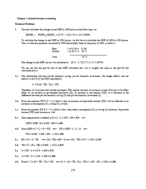
Chapter 2 national income accountingTechnical Problems1.The text calculates the change in real GDP in 1996 prices in the following way:[RGDP04 - RGDP96]/RGDP96 = [3.50 - 1.50]/1.50 = 1.33 = 133%.To calculate the change in real GDP in 2004 prices, we first have to calculate the GDP of 1996 in 2004 prices.Thus we take the quantities consumed in 1996 and multiply them by the prices of 2004, as follows:B eer 1 at $2.00 = $2.00Skittles 1 at $0.75 = $0.75_______________________________Total $2.75The change in real GDP can now be calculated as [6.25 - 2.75]/2.75 = 1.27 = 127%.We can see that the growth rate of real GDP calculated this way is roughly the same as the growth rate calculated above.2.a. The relationship between private domestic saving, private domestic investment, the budget deficit, and netexports is shown by the following identity:S - I ≡ (G + TR - TA) + NX.Therefore, if we assume that transfer payments (TR) remain constant, an increase in taxes (TA) has to be offset either by an increase in government purchases (G), an increase in net exports (NX), or a decrease in the difference between private domestic saving (S) and private domestic investment (I).2.b.From the equation YD ≡ C + S it follows that an increase in disposable income (YD) will be reflected in anincrease in consumption (C), saving (S), or both.2.c.From the equation YD ≡ C + S it follows that when either consumption (C) or saving (S) increases, disposableincome (YD) must increase as well.3.a. Since depreciation is defined as D = I g - I n = 800 - 200 = 600 ==>NDP = GDP - D = 6,000 - 600 = 5,400.3.b.From GDP = C + I g + G + NX ==> NX = GDP - C – I g - G ==>NX = 6,000 - 4,000 - 800 - 1,100 = 100.3.c.BS = TA - G - TR ==> (TA - TR) = BS + G ==> (TA - TR) = 30 + 1,100 = 1,1303.d.YD = Y - (TA - TR) = 6,000 - 1,130 = 4,8703.e. S = YD - C = 4,870 - 4,000 = 8704.a. S = YD - C = 5,100 - 3,800 = 1,3004.b.From S - I = (G + TR - TA) + NX ==> I = S - (G + TR - TA) - NX = 1,300 - 200 - (-100) = 1,200.2704.c.From Y = C + I + G + NX ==> G = Y - C - I - NX ==>G = 6,000 - 3,800 - 1,200 - (-100) = 1,100.Also: YD = Y - TA + TR ==> TA - TR = Y - YD = 6,000 - 5,100 ==> TA - TR = 900From BS = TA - TR - G ==> G = (TA - TR) - BS = 900 - (-200) ==> G = 1,100.5.According to Equation (2) in the text, the value of total output (in billions of dollars) can be calculated as: Y =labor payments + capital payments + profits = $6 + $2 + $0 = $8.6.a.Since nominal GDP is defined as the market value of all final goods and services currently produced in thiscountry, we can only measure the value of the final product (bread), and therefore we get $2 million (since 1 million loaves are sold at $2 each).6.b.An alternative way of measuring GDP is to calculate all the value added at each step of production. The totalvalue of the ingredients used by the bakeries can be calculated as:1,200,000 pounds of flour ($1 per pound) = 1,200,000100,000 pounds of yeast ($1 per pound) = 100,000100,000 pounds of sugar ($1 per pound) = 100,000100,000 pounds of salt ($1 per pound) = 100,000__________________________________________________________= 1,500,000Since $2,000,000 worth of bread is sold, the total value added at the bakeries is $500,000.7.If the CPI increases from 2.1 to 2.3, the rate of inflation can be calculated in the following way:rate of inflation = (2.3 - 2.1)/2.1 = 0.095 = 9.5%.The CPI often overstates inflation, since it is calculated by using a fixed market basket of goods and services.But the fixed weights in the CPI's market basket cannot capture the tendency of consumers to substitute away from goods whose relative prices have increased. Quality improvements in goods also often are not adequately taken into account. Therefore, the CPI will overstate the increase in consumers' expenditures.8.The real interest rate (r) is defined as the nominal interest rate (i) minus the rate of inflation (π). Therefore thenominal interest rate is the real interest rate plus the rate of inflation, ori = r + π = 3% + 4% = 7%.Chapter 3Growth theory, exogenous.1.a.According to Equation (2), the growth of output is equal to the growth in lab or times labor’s share ofincome plus the growth of capital times capital’s share of income plus the rate of technical progress, that is,∆Y/Y = (1 - θ)(∆N/N) + θ(∆K/K) + ∆A/A, where2711 - θ is the share of labor (N) and θ is the share of capital (K). Therefore, if we assume that therate of technological progress is zero (∆A/A = 0), output grows at an annual rate of 3.6 percent, since ∆Y/Y = (0.6)(2%) + (0.4)(6%) + 0% = 1.2% + 2.4% = + 3.6%,1.b.The so-called "Rule of 70" suggests that the length of time it takes for output to double can becalculated by dividing 70 by the growth rate of output. Since 70/3.6 = 19.44, it will take just under 20 years for output to double at an annual growth rate of 3.6%,1.c.Now that ∆A/A = 2%, we can calculate economic growth as∆Y/Y = (0.6)(2%) + (0.4)(6%) + 2% = 1.2% + 2.4% + 2% = + 5.6%.Thus it will take 70/5.6 = 12.5 years for output to double at this new growth rate of 5.6%.2.a.According to Equation (2), the growth of output is equal to the growth in labor times the labor shareplus the growth of capital times the capital share plus the growth rate of total factor productivity, that is,∆Y/Y = (1 - θ)(∆N/N) + θ(∆K/K) + ∆A/A, where1 - θ is the share of labor (N) and θ is the share of capital (K). In this example θ = 0.3; therefore,if output grows at 3% and labor and capital grow at 1% each, we can calculate the change in total factor productivity in the following way3% = (0.7)(1%) + (0.3)(1%) + ∆A/A ==> ∆A/A = 3% - 1% = 2%,that is, the growth rate of total factor productivity is 2%.2.b.If both labor and the capital stock are fixed, that is, ∆N/N = ∆K/K = 0, and output grows at 3%, thenall the growth has to be contributed to the growth in total factor productivity, that is, ∆A/A = 3%.3.a.If the capital stock grows by ∆K/K = 10%, the effect on output will be an additional growth rate of∆Y/Y = (0.3)(10%) = 3%.3.b.If labor grows by ∆N/N = 10%, the effect on output will be an additional growth rate of∆Y/Y = (0.7)(10%) = 7%.3.c.If output grows at ∆Y/Y = 7% due to an increase in labor by ∆N/N = 10% and this increase in labor isentirely due to population growth, then per-capita income will decrease and people’s welfare will decrease, since∆y/y = ∆Y/Y - ∆N/N = 7% - 10% = - 3%.2723.d.If the increase in labor is due to an influx of women into the labor force, the overall population doesnot increase, and income per capita will increase by y/y = 7%. Therefore people's welfare (or at least their living standard) will increase.4.Figure 3-4 shows output per head as a function of the capital-labor ratio, that is, y = f(k). Thesavings function is sy = sf(k) and it intersects the (n + d)k-line, representing the investment requirement. At this intersection, the economy is in a steady-state equilibrium. Now let us assume that the economy is in a steady-state equilibrium before the earthquake hits, that is, the capital-labor ratio is currently k*. Assume further, for simplicity, that the earthquake does not affect pe oples’ savings behavior.If the earthquake destroys one quarter of the capital stock but less than one quarter of the labor force, then the capital-labor ratio will fall from k* to k1 and per-capita output will fall from y* to y1.Now saving is greater than the investment requirement, that is, sy1 > (d + n)k1, and the capital stock and the level of output per capita will grow until the steady state at k* is reached again.However, if the earthquake destroys one quarter of the capital stock but more than one quarter of the labor force, then the capital-labor ratio will increase from k* to k2. Saving (and gross investment) now will be less than the investment requirement and thus the capital-labor ratio and the level of output per capita will fall until the steady state at k* is reached again.If exactly one quarter of both the capital stock and the labor stock are destroyed, then the steady state will be maintained, that is, the capital-labor ratio and the output per capita will not change.If the severity o f the earthquake has an effect on peoples’ savings behavior, the savings function sy = sf(k) will move either up or down, depending on whether the savings rate (s) increases (if people save more, so more can be invested in an effort to rebuild) or decreases (if people save less, since they decide that life is too short not to live it up). But in either case, a new steady-state equilibrium will be reached.k1k k2 k5.a.An increase in the population growth rate (n) affects the investment requirement. As n gets larger, the(n + d)k-line gets steeper. As the population grows, increases in saving and investment will be required to equip new workers with the same amount of capital that existing workers already have.273Since the population will now be growing faster than output, income per capita (y) will decrease anda new optimal capital-labor ratio will be determined by the intersection of the sy-curve and the new(n1 + d)k-line. Since per-capita output will fall, we will have a negative growth rate in the short run.However, the steady-state growth rate of output will increase in the long run, since it will be determined by the new and higher rate of population growth.y oy1k1k o k5.b.Starting from an initial steady-state equilibrium at a level of per-capita output y*, the increase in thepopulation growth rate (n) will cause the capital-labor ratio to decline from k* to k1. Output per capita will also decline, a process that will continue at a diminishing rate until a new steady-state level is reached at y1. The growth rate of output will gradually adjust to the new and higher level n1.yy*y1t o t1tkk*k1t o t1t6.a.Assume the production function is of the formY = F(K, N, Z) = AK a N b Z c==>274∆Y/Y = ∆A/A + a(∆K/K) + b(∆N/N) + c(∆Z/Z), with a + b + c = 1.Now assume that there is no technological progress, that is, ∆A/A = 0, and that capital and labor grow at the same rate, that is, ∆K/K = ∆N/N = n. If we also assume that all available natural resources are fixed, such that ∆Z/Z = 0, then the rate of output growth will be∆Y/Y = an + bn = (a + b)n.In other words, output will grow at a rate less than n since a + b < 1, and output per worker will fall.6.b.If there is technological progress, that is, ∆A/A > 0, then output will grow faster than before, namely∆Y/Y = ∆A/A + (a + b)n.If ∆A/A < cn, output will grow at a lower rate than n, in which case output per worker will still decrease.If ∆A/A = cn, output will grow at the same rate as n, in which case output per worker will remain the same.But if ∆A/A > cn, output will grow at a rate higher than n, in which case output per worker will increase.6.c.If the supply of natural resources is fixed, then output can only grow at a rate that is smaller than therate of population growth and we should expect limits to growth as we run out of natural resources.However, if the rate of technological progress is sufficiently large, then output can grow at a rate faster than population, even if we have a fixed supply of natural resources.7.a.If the production function is of the formY = K1/2(AN)1/2,and A is normalized to 1, we haveY = K1/2N1/2 .In this case, capital's and labor's shares of income are both 50%.7.b.This is a Cobb-Douglas production function.7.c. A steady-state equilibrium is reached when sy = (n + d)k.From Y = K1/2N1/2 ==> Y/N = K1/2N-1/2==> y = k1/2 ==> sk1/2 = (n + d)k==> k-1/2 = (n + d)/s = (0.07 + 0.03)/(.2) = 1/2 ==> k1/2 = 2 = y ==> k = 4 .7.d.At the steady-state equilibrium, output per capita remains constant, since total output grows at thesame rate as the population (7%), as long as there is no technological progress, that is, ∆A/A = 0. But275if total factor productivity grows at ∆A/A = 2%, then total output will grow faster than population, that is, at 7% + 2% = 9%, so output per capita will grow at 2%.8.a.If technological progress occurs, then the level of output per capita for any given capital-labor ratioincreases. The function y = f(k) increases to y = g(k), and thus the savings function increases from sf(k) to sg(k).8.b.Since g(k) > f(k), it follows that sg(k) > sf(k) for each level of k. Therefore, the intersection of thesg(k)-curve with the (n + d)k-line is at a higher level of k. The new steady-state equilibrium will now be at a higher level of saving and output per capita, and at a higher capital-labor ratio.8.c.After the technological progress occurs, the level of saving and investment will increase until a newand higher optimal capital-labor ratio is reached. The investment ratio will increase in the transition period, since more investment will be required to reach the higher optimal capital-labor ratio.9.The Cobb-Douglas production function is defined asY = F(N, K) = AN1-θKθ.The marginal product of labor can then be derived asMP N = (∆Y)/(∆N) = (1 - θ)AN-θKθ = (1 - θ)AN1-θKθ/N = = (1 - θ)(Y/N)== > labor's share of income = [MP N*N]/Y = [(1 - θ)(Y/N)](N/Y) = (1 - θ).Chapter 4Growth theory, endogenous1.a. A production function that displays both a diminishing and a constant marginal product of capital canbe displayed by drawing a curved line (as in an exogenous growth model), followed by an upward-sloping line (as in an endogenous growth model). Such a graph is depicted below.1.b.The first equilibrium (Point A in the graph below) is a stable low-income steady-state equilibrium.Any deviation from that point will cause the economy to eventually adjust again at the same steady-state income level (and capital-output ratio). The second equilibrium (Point B) is an unstable high-income steady-state equilibrium. Any deviation from that point will lead to either a lower income steady-state equilibrium back at Point A (if the capital-labor ratio declines) or ongoing growth (if the capital-labor ratio increases). In the latter case, not only total output but also output per capita continues to grow.1.c. A model like the one in this question can be used to explain how some countries find themselves insituations with no growth and low income while others have ongoing growth and a high level of income. In the first case, a country may have invested mostly in physical capital, leading to some short-term growth at the expense of long-term growth. In the second case, a country may have invested not only in physical capital but also in human capital (education, skills, and training), reaping significant social returns.2762.a.If population growth is endogenous, that is, if a country can influence the rate of population growththrough government policies, then the investment requirement is no longer a straight line. Instead it is curved as depicted below.2.b.The first equilibrium (Point A) is a stable steady-state equilibrium. This is a situation of low incomeand high population growth, indicating that the country is in a poverty trap. The second equilibrium (Point B) is an unstable steady-state equilibrium. This is a situation of medium income and low population growth. The third equilibrium (Point C) is a stable steady-state equilibrium. This is a situation of high income and low population growth. In none of these three cases do we have ongoing growth. For any capital stock k < k B, the economy will adjust to k A, but for any capital stock k > k b (even for k > k c), the economy will adjust to k B. During the adjustment process to any of these two steady-state equilibria, the change in output per capita only will be transitory.2.c.To escape the poverty trap (Point A), a country has several possibilities: First, it can somehow find themeans to increase the capital-labor ratio above a level consistent with Point B (perhaps by borrowing funds or seeking direct foreign investment). Second, it can increase the savings rate such that the savings function no longer intersects the investment requirement curve at either Point A or Point B.Third, it can decrease the rate of population growth through specifically designed policies, such that the investment requirement shifts down and no longer intersects with the savings function at Points A or B.3.a.If we incorporate endogenous population growth into a two-sector model in Problem 2, we get acurved investment requirement line and a production function with first a diminishing and then a constant marginal product of capital as depicted below. (Note that the savings function has the same shape as the production function.)3.b. Here we should have four intersections of the savings function sf(k) and the investment requirement[n(y)+d]k. The first equilibrium (at Point A) is a stable low-income steady-state equilibrium. Any deviation from that point will cause the economy to eventually adjust again at the same steady-state income level (and capital-output ratio). The second equilibrium (at Point B) is an unstable low-income equilibrium. Any deviation from that point will lead to either a lower income steady-state equilibrium at Point A (if the capital-labor ratio declines) or a higher income steady-state equilibrium at Point C (if the capital-labor ratio increases). Since Point C is a stable equilibrium, the economy will settle back at that point again whether the capital stock increases or declines. Point D is again an unstable equilibrium but at a high level of income. Any deviation from that point will lead to either a lower income steady-state equilibrium at Point C (if the capital-labor ratio declines) or ongoing growth (if the capital-labor ratio increases).3.c.This model is more inclusive than either of the two models discussed previously and therefore hasgreater explanatory power. While the graphical analysis is far more complicated, we can now see more clearly that a poor country cannot escape the poverty trap at Point A unless it somehow succeeds in increasing the capital-labor ratio (and thus per-capita income) beyond the level at Point B.4.a.The production function is of the formY = K1/2(AN)1/2 = K1/2(4[K/N]N)1/2= K1/2(4K)1/2 = 2K.From this we can see that a = 2 since277Y = Y/N = 2(K/N) == > y = 2k.4.b.Since a = y/k = 2, it follows that the growth rate of output and capital is∆y/y = ∆k/k = g = sa - (n + d) = (0.1)2 - (0.02 + 0.03) = 0.15 = 15%.4.c.The term "a" in the equation above stands for the marginal product of capital. By assuming that thelevel of labor-augmenting technology (A) is proportional to the capital-labor ratio (k), it is implied that the level of technology depends on the amount of capital per worker that we have, which may not be realistic.4.d.In this model, we have a constant marginal product of capital and therefore we have an endogenousgrowth model.5.a.The production function is of the formY = K1/2N1/2==> Y/N = (K/N)1/2 ==> y = k1/2.From k = sy/(n + d) = sk1/2/(n +d) ==> k1/2 = s/(n + d)==> y* = s/(n + d) = (0.1)/(0.02 + 0.03) = 2==> k* = sy*/(n + d) = (0.1)(2)/(0.02 + 0.03) = 4.5.b.Steady-state consumption equals steady-state income minus steady-state saving (or investment), thatis,c* = y – sy = f(k*) - (n + d)k* .The golden-rule capital stock corresponds to the highest permanently sustainable level of consumption. Steady-state consumption is maximized when the marginal increase in capital produces just enough extra output to cover the increased investment requirement.From c = k1/2 - (n + d)k ==> (∆c/∆k) = (1/2)k-1/2 - (n + d) = 0==> k-1/2 = 2(n + d) = 2(.02 + .03) = .1==> k1/2 = 10 ==> k = 100.Since k* = 4 < 100, we have less capital at the steady state than the golden rule suggests.5.c.From k = sy/(n + d) = sk1/2/(n + d) ==> s = k1/2(n + d) = 10(0.05) = 0.5.5.d.If we have more capital than the golden rule suggests, we are saving too much and do not have theoptimal amount of consumption.Chapter 9Income and spending2781.a. AD = C + I = 100 + (0.8)Y + 50 = 150 + (0.8)YThe equilibrium condition is Y = AD ==>Y = 150 + (0.8)Y ==> (0.2)Y = 150 ==> Y = 5*150 = 750.1.b.Since TA = TR = 0, it follows that S = YD - C = Y - C. ThereforeS = Y - [100 + (0.8)Y] = - 100 + (0.2)Y ==> S = - 100 + (0.2)750 = - 100 + 150 = 50.As we can see S = I, which means that the equilibrium condition is fulfilled.1.c.If the level of output is Y = 800, then AD = 150 + (0.8)800 = 150 + 640 = 790.Therefore the amount of involuntary inventory accumulation is UI = Y - AD = 800 - 790 =10.1.d. AD' = C + I' = 100 + (0.8)Y + 100 = 200 + (0.8)YFrom Y = AD' ==> Y = 200 + (0.8)Y ==> (0.2)Y = 200 ==> Y = 5*200 = 1,000Note: This result can also be achieved by using the multiplier formula:∆Y = (multiplier)(∆Sp) = (multiplier)(∆I) ==> ∆Y = 5*50 = 250,that is, output increases from Y o = 750 to Y1 = 1,000.1.e.From 1.a. and 1.d. we can see that the multiplier is α = 5.2.a.Since the mpc has increased from 0.8 to 0.9, the size of the multiplier is now larger. Therefore weshould expect a higher equilibrium income level than in 1.a.AD = C + I = 100 + (0.9)Y + 50 = 150 + (0.9)Y ==>Y = AD ==> Y = 150 + (0.9)Y ==> (0.1)Y = 150 ==> Y = 10*150 = 1,500.2.b.From ∆Y = (multiplier)(∆I) = 10*50 = 500 ==> Y1 = Y o + ∆Y = 1,500 + 500 = 2,000.2.c.Since the size of the multiplier has doubled from α = 5 to α1 = 10, the change in output (Y) that resultsfrom a change in investment (I) now has also doubled from 250 to 500.3.a. AD = C + I + G + NX = 50 + (0.8)YD + 70 + 200 + 0 =320 + (0.8)[Y - TA + TR]= 320 + (0.8)[Y - (0.2)Y + 100] = 400 + (0.8)(0.8)Y = 400 + (0.64)YFrom Y = AD ==> Y = 400 + (0.64)Y ==> (0.36)Y = 400279==> Y = (1/0.36)400 = (2.78)400 = 1,111.11The size of the multiplier is α = 1/0.36) = 2.78.3.b.BS = tY - TR - G = (0.2)(1,111.11) - 100 - 200 = 222.22 - 300 = - 77.783.c.AD' = 320 + (0.8)[Y - (0.25)Y + 100] = 400 + (0.8)(0.75)Y = 400 + (0.6)YFrom Y = AD' ==> Y = 400 + (0.6)Y ==> (0.4)Y = 400 ==> Y = (2.5)400 = 1,000The size of the multiplier is now reduced to α1 = (1/0.4) = 2.5.3.d.The size of the multiplier and equilibrium output will both increase with an increase in the marginalpropensity to consume. Therefore income tax revenue will also go up and the budget surplus should increase. This can be seen as follows:BS' = (0.25)(1,000) - 100 - 200 = - 50 ==> BS' - BS = - 50 - (-77.78) = + 27.783.e.If the income tax rate is t = 1, then all income is taxed. There is no induced spending and equilibriumincome always increases by exactly the change in autonomous spending. In other words, the size of the expenditure multiplier is 1.From Y = C + I + G ==> Y = C o + c(Y - TA + TR) + I o + G o = C o + c(Y - 1Y + TR o) + I o + G o ==> Y = C o + cTR o + I o + G o = A o==> ∆Y = ∆A o4.On first sight, one may want to conclude that this is an application of the balanced budget theorem,since, as long as Y = 1,000, a change in the tax rate by 5% will cause total tax revenues to change by ∆TA = 50, which is the same as the change in government purchases, that is, ∆G = 50. As long as income (Y) stays the same, the budget surplus will not be affected. However, this combined fiscal policy change will have an effect on national income and, since national income goes up, so does the government’s tax revenue, due to the fact that we have income taxation. Therefore we should expect an increase in the budget surplus. This can easily be shown with a numerical example.For example, in Problem 3.d. we had a situation where the following was given:Y o = 1,000, t o = 0.25, G o = 200 and BS o = - 50.Assume now that t1 = 0.3 and G1 = 250 ==>AD' = 50 + (0.8)[Y - (0.3)Y + 100] + 70 + 250 = 370 + (0.8)(0.7)Y + 80 = 450 + (0.56)Y.From Y = AD' ==> Y = 450 + (0.56)Y ==> (0.44)Y = 450==> Y = (1/0.44)450 = 1,022.73280BS1 = (0.3)(1,022.73) - 100 - 250 = 306.82 - 350 = - 43.18 == > BS1– BS o = -43.18 - (-50) = + 6.82Therefore we see that the budget surplus has increased, since the increase in income tax revenue is larger than the increase in government purchases.5.a.While an increase in government purchases by ∆G = 10 will change intended spending by ∆Sp = 10,a decrease in government transfers by ∆TR = -10 will change intended spending by a smaller amount,that is, by only ∆Sp = c(∆TR) = c(-10). The change in intended spending equals ∆Sp = (1 - c)(10) and equilibrium income should therefore increase by∆Y = (multiplier)(1 - c)10.5.b.If c = 0.8 and t = 0.25, then the size of the multiplier isα = 1/[1 - c(1 - t)] = 1/[1 - (0.8)(1 - 0.25)] = 1/[1 - (0.6)] = 1/(0.4) = 2.5.The change in equilibrium income is∆Y = α(∆A o) = α[∆G + c(∆TR)] = (2.5)[10 + (0.8)(-10)] = (2.5)2 = 55.c.The budget surplus should increase, since the level of equilibrium income has increased and thereforethe level of tax revenues has increased, while the changes in government purchases and transfer payments cancel each other out. Numerically, this can be shown as follows:∆BS = t(∆Y) - ∆TR - ∆G = (0.25)(5) - (-10) - 10 = 1.25Chapter 10Money, interest, fiscal policy1.a. Each point on the IS-curve represents an equilibrium in the expenditure sector. (Note that this is aclosed economy, that is, NX = 0).The IS-curve can be derived by setting actual income equal to intended spending, orY = C + I + G = (0.8)[1 - (0.25)]Y + 900 - 50i + 800 = 1,700 + (0.6)Y - 50i ==>(0.4)Y = 1,700 - 50i ==> Y = (2.5)(1,700 - 50i) ==> Y = 4,250 - 125i.1.b.The IS-curve shows all combinations of the interest rate and output level such that the expendituresector (the goods market) is in equilibrium, that is, actual output equals intended spending. A decrease in the interest rate stimulates investment spending, making intended spending greater than actual output. The resulting unintended inventory decrease leads firms to increase their production until actual output is again equal to intended spending. This means that the IS-curve is downward sloping.1.c.Each point on the LM-curve represents an equilibrium in the money sector. Therefore the LM-curvecan be derived by setting real money supply equal to real money demand, that is,281M/P = L ==> 500 = (0.25)Y - 62.5i ==> Y = 4(500 + 62.5i) ==> Y = 2,000 + 250i.1.d.The LM-curve shows all combinations of the interest rate and level of output such that the moneysector is in equilibrium, that is, the demand for real money balances is equal to the supply of real money balances. An increase in income will increase the demand for real money balances. Given a fixed real money supply, this will lead to an increase in interest rates, which will then reduce the quantity of real money balances demanded until the money market clears again. In other words, the LM-curve is upward sloping.1.e.The level of income (Y) and the interest rate (i) at the equilibrium are determined by the intersectionof the IS-curve with the LM-curve. At this point, the expenditure sector and the money sector are both in equilibrium simultaneously.From IS = LM ==> 4,250 - 125i = 2,000 + 250i ==> 2,250 = 375i ==> i = 6==> Y = 4,250 - 125*6 = 4,250 - 750 ==> Y = 3,500Check: Y = 2,000 + 250*6 = 2,000 + 1,500 = 3,500i125 ISLM62,000 3,500 4,250 Y2.a.As we have seen in 1.a., the value of the expenditure multiplier is α = 2.5. This multiplier is derivedin the same way as in Chapter 9. But now intended spending also depends on the interest rate, so we no longer have Y = αA o, but ratherY = α(A o - bi) = (1/[1 - c + ct])(A o - bi) ==> Y = (2.5)(1,700 - 50i) = 4,250 - 125i.2.b.In the IS-LM model, an increase in government purchases (G) will have a smaller effect on outputthan in the model of the expenditure sector used in Chapter 9, in which interest rates are assumed to be fixed. This can be answered most easily with a numerical example. Assume that government purchases increase by ∆G = 300. The IS-curve shifts parallel to the right by==> ∆IS = (2.5)(300) = 750.Therefore, the equation of the new IS-curve is: Y = 5,000 - 125i.282。
多恩布什宏观经济学课后答案【篇一:宏观经济学课后习题答案】> 1、我们将本章阐述的收入决定模型叫做凯恩斯模型。
什么原因使得凯恩斯模型成为古典模型的对立面呢?在凯恩斯模型中价格水平是假定不变的,也就是说总供给曲线是水平的,产出由总需求唯一的决定。
而另一方面,在古典模型中,价格完全取决于充分就业下的产出水平,也就是说总供给曲线是竖直的。
而由于本章中的收入决定模型所做的假设是价格水平是固定的,与凯恩斯模型的假设相同,所以我们使用凯恩斯模型,凯恩斯模型也因此成为古典模型的对立面。
2、什么是自主性变量?在本章中,我们规定总需求中那些组成部分是自主性的?自主性变量是外生变量,由模型以外的东西决定。
本章中我们假设:总需求的自主性开支(autonomous spending—c*)、自主性投资(autonomous investment—i0)、政府购买(government purchases—g0)、税收(taxes—ta)、转移支付(transfer payments—tr)、净出口(net export—nx)是自主性的。
3、根据你对于联邦政府许多部门同意并实施政策变动所需时间的了解,你能想到有关财政政策稳定经济的任何问题么?对于经济学家和政客们来说,在某一经济问题上达成共识很困难,因此一项政策的决定常常需要很长时间。
在这段时间里,经济很可能发生巨大的变动。
如果在经济衰退过后已经出现快速增长趋势的时候才决定好通过减税改善前一段时间的经济状况,那么,毫无疑问,这一过时的政策会导致通货膨胀,起到完全相反的作用。
4、为什么将比例税所得与福利制度等机制成为自动稳定器?选择其中一个稳定器,详细解释它如何并且为什么会影响产出波动。
自动稳定器是经济中的一种机制,它会自动减少为适应自主性需求变动所需要的产出变动量而不需要政府一步步具体地加以干预。
当自动稳定器处于适当状态时,投资需求的变动对产出的影响会变小。
这意味着自动稳定器的存在使我们期望产出波动可以比没有这些自动稳定器时的幅度减小。
多恩布什宏观经济学第⼗⼆版课后答案完整版多恩布什《宏观经济学》(第12版)笔记和课后习题详解内容简介知择学习⽹的多恩布什《宏观经济学》(第12版)笔记和课后习题详解严格按照教材内容进⾏编写,遵循教材第12版的章⽬编排,共分24章,每章由两部分组成:第⼀部分为复习笔记,总结本章的重难点内容;第⼆部分是课(章)后习题详解,对第12版的所有习题都进⾏了详细的分析和解答。
⽬录第1章导论1.1 复习笔记1.2 课后习题详解第2章国民收⼊核算2.1 复习笔记2.2 课后习题详解第3章增长与积累3.1 复习笔记3.2 课后习题详解第4章增长与政策4.1 复习笔记4.2 课后习题详解第5章总供给与总需求5.1 复习笔记5.2 课后习题详解第6章总供给和菲利普斯曲线6.1 复习笔记6.2 课后习题详解第7章失业7.1 复习笔记7.2 课后习题详解第8章通货膨胀8.1 复习笔记8.2 课后习题详解第9章政策预览9.1 复习笔记9.2 课后习题详解第10章收⼊与⽀出10.1 复习笔记10.2 课后习题详解第11章货币、利息与收⼊11.1 复习笔记11.2 课后习题详解第12章货币政策与财政政策12.1 复习笔记12.2 课后习题详解第13章国际联系13.1 复习笔记13.2 课后习题详解第14章消费与储蓄14.1 复习笔记14.2 课后习题详解第15章投资⽀出15.1 复习笔记15.2 课后习题详解第16章货币需求16.1 复习笔记16.2 课后习题详解第17章联邦储备、货币与信⽤17.1 复习笔记17.2 课后习题详解第18章政策18.1 复习笔记18.2 课后习题详解第19章⾦融市场与资产价格19.1 复习笔记19.2 课后习题详解第20章国家债务20.1 复习笔记20.2 课后习题详解第21章衰退与萧条21.1 复习笔记21.2 课后习题详解第22章通货膨胀与恶性通货膨胀22.1 复习笔记22.2 课后习题详解第23章国际调整与相互依存23.1 复习笔记23.2 课后习题详解第24章前沿课题24.1 复习笔记24.2 课后习题详解内容第2章国民收⼊核算2.2 课后习题详解⼀、概念题1.经过调整的GNP( ( adjusted GNP)答:经过调整的GNP指以具有不变购买⼒的货币单衡量的国民⽣产总值。