泰勒公式外文翻译

泰勒定理和泰勒公式
泰勒定理（Taylor's theorem）是一个数学定理，描述了一个实数或复数函数在某个点附近的函数值与它在该点处的函数值及各阶导数之间的关系。

泰勒公式（Taylor series）是泰勒定理的一个特例，表达了一个实数或复数函数在某个点附近的函数值为无限次可导函数在该点处的函数值及各阶导数的线性组合。

泰勒公式的一般形式如下：
f(x) = f(a) + f'(a)(x-a) + f''(a)(x-a)^2/2! + f'''(a)(x-a)^3/3! + ...
其中，f(x)表示要近似的函数，f(a)表示函数在某个点a处的函数值，f'(a)、f''(a)、f'''(a)等表示函数在点a处的一阶、二阶、三阶导数，(x-a)表示自变量和点a之间的差值，n!表示n的阶乘。

公式右侧的无穷级数表示了函数在点a处的各阶导数对函数值的贡献。

泰勒公式在数学和工程中广泛应用，能够以多项式逼近复杂函数，帮助简化计算和分析。

简介在数学上, 一个定义在开区间(a-r, a+r)上的无穷可微的实变函数或复变函数f的泰勒级数是如下的幂级数这里，n!表示n的阶乘而f?(n)(a) 表示函数f在点a处的n阶导数。

如果泰勒级数对于区间(a-r, a+r)中的所有x都收敛并且级数的和等于f(x)，那么我们就称函数f(x)为解析的。

当且仅当一个函数可以表示成为幂级数的形式时，它才是解析的。

为了检查级数是否收敛于f(x)，我们通常采用泰勒定理估计级数的余项。

上面给出的幂级数展开式中的系数正好是泰勒级数中的系数。

如果a = 0, 那么这个级数也可以被称为麦克劳伦级数。

泰勒级数的重要性体现在以下三个方面：首先，幂级数的求导和积分可以逐项进行，因此求和函数相对比较容易。

第二，一个解析函数可被延伸为一个定义在复平面上的一个开片上的解析函数，并使得复分析这种手法可行。

第三，泰勒级数可以用来近似计算函数的值。

对于一些无穷可微函数f(x) 虽然它们的展开式收敛，但是并不等于f(x)。

例如，分段函数f(x) = exp(?1/x2) 当x≠ 0 且f(0) = 0 ，则当x = 0所有的导数都为零，所以这个f(x)的泰勒级数为零，且其收敛半径为无穷大，虽然这个函数f仅在x = 0 处为零。

而这个问题在复变函数内并不成立，因为当z沿虚轴趋于零时 exp(? 1/z2) 并不趋于零。

一些函数无法被展开为泰勒级数因为那里存在一些奇点。

但是如果变量x是负指数幂的话，我们仍然可以将其展开为一个级数。

例如，f(x) = exp(?1/x2) 就可以被展开为一个洛朗级数。

Parker-Sockacki theorem是最近发现的一种用泰勒级数来求解微分方程的定理。

这个定理是对Picard iteration一个推广。

[编辑]泰勒级数列表下面我们给出了几个重要的泰勒级数。

它们对于复参数x依然成立。

指数函数和自然对数:几何级数:二项式定理:三角函数:双曲函数:Lambert's W function:tan(x) 和 tanh(x) 展开式中的B k是Bernoulli numbers。

数学专业外文翻译---幂级数的展开及其应用In the us n。

we XXX its convergence n。

a power series always converges to a n。

We can use simple power series。

as well as XXX quadrature methods。

to find this n。

However。

this n will address another issue: can an arbitrary n f(x) be expanded into a power series?XXX n will address this XXX power series can be seen as an n of reality。

so we can start to solve the problem of expanding a n f(x) into a power series by considering f(x) and polynomials。

To do this。

we will introduce the following formula without proof:Taylor'XXX that if a n f(x) has derivatives of order n+1 in a neighborhood of x=x0.then we can use the following XXX:f(x)=f(x0)+f'(x0)(x-x0)+f''(x0)(x-x0)^2+。

+f^(n)(x0)(x-x0)^n+r_n(x)Here。

r_n(x) represents the remainder term.XXX (x) is given by (x-x)n+1.This formula is of the (9-5-1) type for the Taylor series。

泰勒公式外文翻译Taylor's Formula and the Study of Extrema1. Taylor's Formula for MappingsTheorem 1. If a mapping Y U f →: from a neighborhood ()x U U = of a point x in a normed space X into a normed space Y has derivatives up to order n -1 inclusive in U and has an n-th order derivative ()()x f n at the point x, then()()()()()⎪⎭⎫ ⎝⎛++++=+n n n h o h x f n h x f x f h x f !1,Λ (1) as 0→h .Equality (1) is one of the varieties of Taylor's formula, written here for rather generalclasses of mappings.Proof. We prove Taylor's formula by induction.For 1=n it is true by definition of ()x f ,.Assume formula (1) is true for some N n ∈-1.Then by the mean-value theorem, formula (12) of Sect. 10.5, and the induction hypothesis, we obtain.()()()()()()()()()()()()()⎪⎭⎫ ⎝⎛=⎪⎭⎫ ⎝⎛=⎪⎪⎭⎫ ⎝⎛-+++-+≤⎪⎭⎫ ⎝⎛+++-+--<<n n n n n n h o h h o h h x f n h x f x f h x f h x f n h f x f h x f 11,,,,10!11sup !1x θθθθθΛΛ，as 0→h .We shall not take the time here to discuss other versions of Taylor's formula, which are sometimes quite useful. They were discussed earlier in detail for numerical functions. At this point we leave it to the reader to derive them (see, for example, Problem 1 below).2. Methods of Studying Interior ExtremaUsing Taylor's formula, we shall exhibit necessary conditions and also sufficient conditions for an interior local extremum of real-valued functions defined on an open subset of a normed space. As we shall see, these conditions are analogous to the differential conditions already known to us for an extremum of a real-valued function of a real variable.Theorem 2. Let R U f →: be a real-valued function defined on an open set U in a normed space X and having continuous derivatives up to order 11≥-k inclusive in a neighborhood of a point U x ∈ and a derivative ()()x f k of order k at the point x itself.If ()()()0,,01,==-x f x f k Λ and ()()0≠x f k , then for x to be an extremum of the function f it is: necessary that k be even and that the form()()k k h x f be semidefinite,andsufficient that the values of the form ()()k k h x f on the unit sphere 1=h be bounded away from zero; moreover, x is a local minimum if the inequalities()()0>≥δk k h x f ,hold on that sphere, and a local maximum if()()0<≤δk k h x f ,Proof. For the proof we consider the Taylor expansion (1) of f in a neighborhood of x. The assumptions enable us to write()()()()()k k k h h h x f k x f h x f α+=-+!1where ()h α is a real-valued function, and ()0→h α as 0→h .We first prove the necessary conditions.Since ()()0≠x f k , there exists a vector 00≠h on which()()00≠k k h x f . Then for values of the real parameter t sufficiently close to zero,()()()()()()k k k th th th x f k x f th x f 0000!1α+=-+()()()kk k k t h th h x f k ⎪⎭⎫ ⎝⎛+=000!1αand the expression in the outer parentheses has the same sign as()()k k h x f 0. For x to be an extremum it is necessary for the left-hand side (and hence also the right-hand side) of this last equality to be of constant sign when t changes sign. But this is possible only if k is even.This reasoning shows that if x is an extremum, then the sign of the difference ()()x f th x f -+0 is the same as that of ()()k k h x f 0 for sufficiently small t; hence in that case there cannot be two vectors 0h , 1h at which the form ()()x f k assumes values with opposite signs.We now turn to the proof of the sufficiency conditions. For definiteness we consider the case when ()()0>≥δk k h x f for 1=h . Then()()()()()k k k h h h x f k x f h x f α+=-+!1()()()k k k h h h h x f k ⎪⎪⎪⎭⎫ ⎝⎛+⎪⎪⎭⎫ ⎝⎛=α!1 ()k h h k ⎪⎭⎫ ⎝⎛+≥αδ!1and, since ()0→h α as 0→h , the last term in this inequality is positive for all vectors0≠h sufficiently close to zero. Thus, for all such vectors h,()()0>-+x f h x f ,that is, x is a strict local minimum.The sufficient condition for a strict local maximum is verified similiarly.Remark 1. If the space X is finite-dimensional, the unit sphere ()1;x S with center at X x ∈, being a closed bounded subset of X, is compact. Then the continuous function()()()()k k i i i i k k h h x f h x f ⋅⋅∂=ΛΛ11 (a k-form) has both a maximal and a minimal value on ()1;x S . Ifthese values are of opposite sign, then f does not have an extremum at x. If they are both of the same sign, then, as was shown in Theorem 2, there is an extremum. In the latter case, a sufficient condition for an extremum can obviously be stated as the equivalent requirement that the form ()()k k h x f be either positive- or negative-definite.It was this form of the condition that we encountered in studying realvalued functions on n R . Remark 2. As we have seen in the example of functions R R fn →:, the semi-definiteness of the form ()()k k h x f exhibited in the necessary conditions for an extremum is not a sufficient criterion for an extremum.Remark 3. In practice, when studying extrema of differentiable functions one normally uses only the first or second differentials. If the uniqueness and type of extremum are obvious from the meaning of the problem being studied, one can restrict attention to the firstdifferential when seeking an extremum, simply finding the point x where ()0,=x f3. Some ExamplesExample 1. Let ()()R R C L ;31∈ and ()[]()R b a C f ;,1∈. In other words, ()()321321,,,,u u u L u u u α is a continuously differentiable real-valued function defined in 3R and ()x f x α a smooth real-valued function defined on the closed interval []R b a ⊂,.Consider the function()[]()R R b a C F →;,:1 (2)defined by the relation()[]()()f F R b a C f α;,1∈()()()R dx x f x f x L ba ∈=⎰,,, (3) Thus, (2) is a real-valued functional defined on the set of functions ()[]()Rb a C ;,1.The basic variational principles connected with motion are known in physics andmechanics. According to these principles, the actual motions are distinguished among all the conceivable motions in that they proceed along trajectories along which certain functionals have an extremum. Questions connected with the extrema of functionals are central in optimal control theory. Thus, finding and studying the extrema of functionals is a problemof intrinsic importance, and the theory associated with it is the subject of a large area ofanalysis - the calculus of variations. We have already done a few things to make the transition from the analysis of the extrema of numerical functions to the problem of finding andstudying extrema of functionals seem natural to the reader. However, we shall not go deeply into the special problems of variational calculus, but rather use the example of the functional(3) to illustrate only the general ideas of differentiation and study of local extrema considered above.We shall show that the functional (3) is a differentiate mapping and find its differential. We remark that the function (3) can be regarded as the composition of the mappings()()()()()x f x f x L x f F ,1,,= (4)defined by the formula()[]()[]()R b a C R b a C F ;,;,:11→ (5)followed by the mapping[]()()()R dx x g g F R b a C g ba ∈=∈⎰2;,α (6) By properties of the integral, the mapping 2F is obviously linear and continuous, so that its differentiability is clear.We shall show that the mapping 1F is also differentiable, and that()()()()()()()()()()x h x f x f x L x h x f x f x L x h f F ,,3,2,1.,,,∂+∂= (7) for ()[]()R b a C h ;,1∈.Indeed, by the corollary to the mean-value theorem, we can write in the present case()()()i i i u u u L u u u L u u u L ∆∂--∆+∆+∆+∑=32131321332211,,,,,,()()()()()()∆⋅∂-∆+∂∂-∆+∂∂-∆+∂≤<<u L u L u L u L u L u L 3312211110sup θθθθ ()()ii i i u L u u L i ∆⋅∂-+∂≤=≤≤=3,2,110max max 33,2,1θθ (8)where ()321,,u u u u = and ()321,,∆∆∆=∆. If we now recall that the norm()1c f of the function f in ()[]()R b a C ;,1 is ⎭⎬⎫⎩⎨⎧c c f f ,,max (where c f is the maximum absolute value of the function on the closed interval []b a ,), then,setting x u =1, ()x f u =2, ()x f u ,3=, 01=∆, ()x h =∆2, and ()x h ,3=∆, we obtain from inequality (8),taking account of the uniform continuity of the functions ()3,2,1,,,321=∂i u u u L i , on bounded subsets of 3R , that()()()()()()()()()()()()()()()()x h x f x f x L x h x f x f x L x f x f x L x h x f x h x f x L b x ,,3,2,,,0,,,,,,,,max ∂-∂--++≤≤ ()()1c h o = as ()01→c h But this means that Eq. (7) holds.By the chain rule for differentiating a composite function, we now conclude that thefunctional (3) is indeed differentiable, and()()()()()()()()()()⎰∂+∂=badx x h x f x f x L x h x f x f x L h f F ,,3,2,,,,, (9) We often consider the restriction of the functional (3) to the affine space consisting of the functions ()[]()R b a C f ;,1∈ that assume fixed values ()A a f =, ()B b f = at the endpoints of the closed interval []b a ,. In this case, the functions h in the tangent space ()1f TC , must have the value zero at the endpoints of the closed interval []b a ,. Taking this fact into account, we mayintegrate by parts in (9) and bring it into the form()()()()()()()()⎰⎪⎭⎫ ⎝⎛∂-∂=b a dx x h x f x f x L dx d x f x f x L h f F ,3,2,,,,, (10) of course under the assumption that L and f belong to the corresponding class ()2C .In particular, if f is an extremum (extremal) of such a functional, then by Theorem 2 we have ()0,=h f F for every function ()[]()R b a C h ;,1∈ such that ()()0==b h a h . From this and relation (10) one can easily conclude (see Problem 3 below) that the function f must satisfy the equation()()()()()()0,,,,,3,2=∂-∂x f x f x L dx d x f x f x L (11)This is a frequently-encountered form of the equation known in the calculus of variations as the Euler-Lagrange equation.Let us now consider some specific examples.Example 2. The shortest-path problemAmong all the curves in a plane joining two fixed points, find the curve that has minimal length.The answer in this case is obvious, and it rather serves as a check on the formalcomputations we will be doing later.We shall assume that a fixed Cartesian coordinate system has been chosen in the plane, in which the two points are, for example, ()0,0 and ()0,1 . We confine ourselves to just the curves that are the graphs of functions ()[]()R C f ;1,01∈ assuming the value zero at both ends of the closed interval []1,0 . The length of such a curve()()()⎰+=102,1dx x f f F (12)depends on the function f and is a functional of the type considered in Example 1. In this case the function L has the form()()233211,,u u u u L +=and therefore the necessary condition (11) for an extremal here reduces to the equation ()()()012,,=⎪⎪⎪⎭⎫ ⎝⎛+x f x f dx d from which it follows that ()()()常数≡+x f x f 2,,1 (13)on the closed interval []1,0Since the function 21u u+ is not constant on any interval, Eq. (13) is possible only if()≡x f ,const on []b a ,. Thus a smooth extremal of this problem must be a linear function whose graph passes through the points ()0,0 and ()0,1. It follows that ()0≡x f , and we arrive at the closed interval of the line joining the two given points.Example 3. The brachistochrone problemThe classical brachistochrone problem, posed by Johann Bernoulli I in 1696, was to find the shape of a track along which a point mass would pass from a prescribed point 0P to another fixed point 1P at a lower level under the action of gravity in the shortest time.We neglect friction, of course. In addition, we shall assume that the trivial case in which both points lie on the same vertical line is excluded.In the vertical plane passing through the points 0P and 1P we introduce a rectangularcoordinate system such that 0P is at the origin, the x-axis is directed vertically downward, and the point 1P has positive coordinates ()11,y x .We shall find the shape of the track among the graphs of smooth functions defined on the closed interval []1,0x and satisfying the condition ()00=f ,()11y x f =. At the moment we shall not take time to discuss this by no meansuncontroversial assumption (see Problem 4 below).If the particle began its descent from the point 0P with zero velocity, the law of variation of its velocity in these coordinates can be written asgx v 2= (14)Recalling that the differential of the arc length is computed by the formula()()()()dx x f dy dx ds 2,221+=+= (15) we find the time of descent()()()⎰+=102,121x dx x x f g f F (16) along the trajectory defined by the graph of the function ()x f y = on the closed interval []1,0x . For the functional (16) ()()1233211,,u u u u u L +=,and therefore the condition (11) for an extremum reduces in this case to the equation ()()()012,,=⎪⎪⎪⎪⎪⎭⎫⎝⎛⎪⎭⎫ ⎝⎛+x f x x f dx d ,from which it follows that ()()()x c x f x f =+2,,1 (17)where c is a nonzero constant, since the points are not both on the same vertical line. Taking account of (15), we can rewrite (17) in the formx c ds dy = (18)However, from the geometric point of viewϕcos =ds dx,ϕsin =ds dy(19)where ϕ is the angle between the tangent to the trajectory and the positive x-axis.By comparing Eq. (18) with the second equation in (19), we find ϕ22sin 1c x = (20) But it follows from (19) and (20) that dx dy d dy =ϕ,2222sin 2sin c c d d tg d dx tg d dx ϕϕϕϕϕϕϕ=⎪⎪⎭⎫⎝⎛==,from which we find()b c y +-=ϕϕ2sin 2212 (21)Setting a c =221and t =ϕ2, we write relations (20) and (21) as()()b t t a y t a x +-=-=sin cos 1 (22)Since 0≠a , it follows that 0=x only for πk t 2=,Z k ∈. It follows from the form of the function(22) that we may assume without loss of generality that the parameter value 0=t corresponds to the point ()0,00=P . In this case Eq. (21) implies 0=b , and we arrive at the simpler form()()t t a y t a x sin cos 1-=-= (23)for the parametric definition of this curve.Thus the brachistochrone is a cycloid having a cusp at the initial point 0P where the tangent is vertical. The constant a, which is a scaling coefficient, must be chosen so that the curve (23) also passes through the point 1P . Such a choice, as one can see by sketching the curve (23), is by no means always unique, and this shows that the necessary condition (11) for an extremum is in general not sufficient. However, from physical considerations it is clear which of thepossible values of the parameter a should be preferred (and this, of course, can be confirmed by direct computation).泰勒公式和极值的研究1.映射的泰勒公式定理1 如果从赋范空间X 的点x 的邻域()x U U =到赋范空间Y 的映射Y U f →:在U 中有直到n-1阶(包括n-1在内)的导数，而在点x 处有n 阶导数。

重庆理工大学文献翻译二级学院数学与统计学院班级 111010101 学生姓名学号 11101010110复杂矩阵用泰勒公式的解决方法一个复杂的R×R矩阵A中的解决方法Rλ（A）是与A的频谱ΣA空交集的任何域名的解析函数。

在任何给定的λ0∉ΣA的附近著名的泰勒展开Rλ（A）的修改考虑到Rλ0只有第一大国（A）是线性无关。

在这个框架的主要工具给出了多变量多项式查看MATHML源取决于不变V1，V2，...，VRRλ（A）的（m为最小多项式的程度）。

这些功能被用于以代表的Rλ0（A）的随后的权力的系数作为它们的第一米的线性组合。

一简介如在[1]中，预解Rλ（A）的≔（λI-A）一种非奇异正方形矩阵A（Ⅰ表示单位矩阵）-1所示的希尔伯特同一性的后果是参数λ的一个解析函数在与A的频谱ΣA因此，空交集的任何域D使用泰勒展开任何固定λ0∈D的附近，我们可以在[1]Rλ（A）的表示公式发现使用Rλ0的一切权力（A）。

在这篇文章中，通过使用一些前面的结果回忆说，例如，在[2]中，我们写下使用Rλ0（A）的权力，只有有限数量的表示公式。

这似乎是因为Rλ0的（A）是线性无关的只有第一个权力是自然的。

在此框架的主要工具是由多变量多项式给出查看MATHML来源（参见[2]，[3]，[4]，[5]和[6]），根据不同的不变量V1，V2，...，vr中的Rλ（A）;这里m表示极小多项式的程度。

二权力矩阵和F k,n功能我们还记得在本节一定的成效上表示公式矩阵的权力（见[2][3][4][5][6]和其参考文献）。

为简单起见，我们指的是情况下，当基质是非贬损使得M = R。

命题2.1。

设A是一个矩阵，由U1表示，U2，...，UR A的不变量，并通过∑=--=-=rj jr j j U A I p 0)1()det()(λλλ其特征多项式（按照惯例u0≔1）;那么对于A 的非负整数指数的权力下表示公式也是如此：Iu u F A u u F A u u F r n r r r n r r n n )...,(...)...,()...,(A 11,211,2111,1-----+++=功能Fk,n(u1...ur)该显示为系数（2.1）由递推关系定义)....,()1(...)....,()....,()....,(1,112,211,11,r r n k r r r n k r n k r n k u u F u u u F u u u F u u u F -----++-=)1;......1(-≥=n rk 和初始条件：)....1,(,).....(,12,1r h k u u F h k r h k r ==-+-δ此外，如果A 是非奇异（ur ≠0），则式（2.1）仍然保持对于n 的负值，只要我们定义FK ，n 功能对于n 的负值如下：)1,......,()...(113,11,rr r r r n k r r n k u u u u u F u u F --+-+-=)1;...1(-<=n r k三 泰勒展开式的解决对策我们认为解决方法矩阵R λ（A ）定义如下：.)(:)(1--=≡A I A R R λλλ注意，有时有标志的公式的变化。

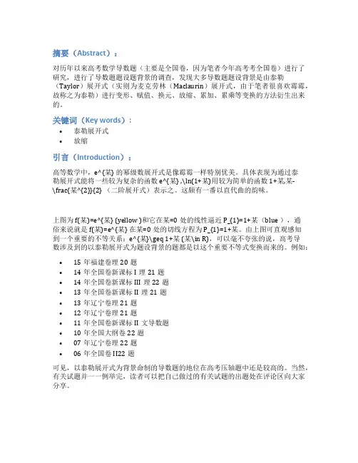
摘要（Abstract）：对历年以来高考数学导数题（主要是全国卷，因为笔者今年高考考全国卷）进行了研究，进行了导数题题设题背景的调查，发现大多导数题题设背景是由泰勒（Taylor）展开式（实则为麦克劳林（Maclaurin）展开式，由于笔者很喜欢霉霉，故称之为泰勒）进行变形、赋值、换元、放缩、累加、累乘等变换的方法衍生出来的。

关键词（Key words）:•泰勒展开式•放缩引言（Introduction）：高等数学中，e^{某} 的幂级数展开式是像霉霉一样特别优美。

具体表现为通过泰勒展开式能将一些较为复杂的函数e^{某} ,\ln(1+某)用较为简单的函数1+某,某-\frac{某^{2}}{2} （二阶展开式）表示之。

这颇有一番以直代曲的韵味。

上图为f(某)=e^{某} (yellow )和它在某=0处的线性逼近P_{1}=1+某（blue ），通俗来说就是f(某)=e^{某} 在某=0处的切线方程为P_{1}=1+某。

由上图可直观感知到一个重要的不等关系：e^{某}\geq 1+某 (某\in R)，可以毫不夸张的说，高考导数涉及到的以泰勒展开式为题设背景的题都是以这个重要不等式变换而来的。

例如：•15年福建卷理20题•14年全国卷新课标I理21题•14年全国卷新课标III理22题•13年全国卷新课标II理21题•13年辽宁卷理21题•12年辽宁卷理21题•11年全国卷新课标II文导数题•10年全国大纲卷22题•07年辽宁卷理22题•06年全国卷II22题可见，以泰勒展开式为背景命制的导数题的地位在高考压轴题中还是较高的。

当然，有关试题并一一例举完，读者可以把自己做过的有关试题的出题处在评论区向大家分享。

在未了解泰勒展开式之前，解决相关导数题时往往采用不等式和导数为工具，进行逻辑推理来解决问题。

正所谓：“会当凌绝顶，一览众山小”，如果没有站在相应高等数学知识的高度，那么很难轻松地看透问题的本质。

摘要泰勒公式是数学分析中的重要组成部分，是一种非常重要的数学工具. 本文通过对泰勒公式的证明方法进行介绍，归纳整理其在求极限与导数、判定级数与广义积分的敛散性、不等式的证明、定积分的证明等方面的应用，从而进一步加深对泰勒公式的认识.关键词：泰勒公式；极限；敛散性；不等式AbstractThe Taylor formula is an important component in mathematical analysis, is also a useful mathematical tool. The paper introduce the proof methods of the Taylor formula, summarize the applications which solve the limit and derivative, judge convergence and divergence of series and generalized integral, the proof of inequality and integral by Taylor formula, thus deeply understand of Taylor formula.Key words: Taylor formula; limit; the property of convergence and divergence; inequality目录摘要 (I)Abstract (II)第1章泰勒公式的概念及其相关理论 (1)第1节泰勒公式的概念及相关理论的证明 (1)第2节常见的初等函数的麦克劳林公式及其推导过程 (5)第2章泰勒公式的应用 (7)第1节利用泰勒公式求极限 (7)第2节利用泰勒公式进行近似计算 (8)第3节利用泰勒公式证明不等式问题 (9)第4节利用泰勒公式判断级数的敛散性 (11)第5节利用泰勒公式证明根的唯一存在性 (12)第6节利用泰勒公式求函数的极值 (13)第7节利用泰勒公式求高阶导数在某些点的数值 (13)第8节利用泰勒公式求初等函数的幂级数展开式 (15)结论 (17)参考文献 (18)致谢 (19)第1章 泰勒公式的概念及其相关理论第1节 泰勒公式的概念及相关理论的证明定义1 若任意的一个函数)(x f （不一定是多项式函数），只要函数)(x f 在a 存在n 阶导数，总能形式的写出相应的n 次多项式n n n a x n a f a x a f a x a f a f x )(!)()(!2)()(!1)()()()(2-++-''+-'+=T （1）则称（1）为函数)(x f 在a 的n 阶泰勒多项式．定义2 若将函数)(x f 与它的n 次泰勒多项式)(x n T 的差表示为)()()(x x f x R n n T -=或)()()(x x R x f n n T +=.)(x R n 为函数)(x f 在a 的n 次泰勒余项，简称泰勒余项．定理1（泰勒定理） 若函数)(x f 在a 存在n 阶导数，则)(a U x ∈∀都有])[()()(n n a x o x x f -+T =,（2） 其中n n n a x n a f a x a f a x a f a f x )(!)()(!2)()(!1)()()()(2-++-''+-'+=T ；)]()[()(a x a x o x R n n →-=，即)(x R n 是比n a x )(-的高阶无穷小.其中)]()[()(a x a x o x R n n →-=称为佩亚诺余项，（2）式成为函数)(x f 在a （展开）的泰勒公式．证法 由高阶无穷小的定义，只需证明0)()()(lim )()(lim=--=-→→nn a x n n a x a x x T x f a x x R ,这是0的待定型，应用1-n 次洛必达法则.证明 )()()(x x f x R n n T -=])(!)()(!2)()(!1)()([)()(2n n a x n a f a x a f a x a f a f x f -++-''+-'+-= . ])()!1()()(!1)()([)()(1)(---++-''+'-'='n n n a x n a f a x a f a f x f x R .])()!2()()(!1)()([)()(2)(---++-''+''-''=''n n n a x n a f a x a f a f x f x R .……)](!1)()([)()()1()1()1(a x a f a fx fx R n n n n n-+-=---.（对它不能再求导数了）当a x →时，显然，)(x R n ，)(x R n '，)(x R n ''，…，)()1(x R n n-，以及)()(+∈-N k a x k 都是无穷小．于是，由洛必达法则有nn a x a x x R )()(lim-→1)()(lim -→-'=n n a x a x n x R 2))(1()(lim-→--''=n na x a x n n x R = )(!)(lim )1(a x n x R n n a x -=-→⎥⎦⎤⎢⎣⎡---=--→)()()(lim !1)()1()1(a f a x a f x f n n n n a x )]()([lim !1)()(a fa f n n n ax -=→0=．定义3 当0=a 时，函数)(x f 在0处存在n 阶导数，（2）式即是)(!)0(!2)0(!1)0()0()()(n nn n x o x n f x f x f f x +++''+'+=T ，称之为麦克劳林公式．定理2（泰勒中值定理） 若函数)(x f 在)(a U 存在1+n 阶导数，)(a U x ∈∀，函数)(t G 在以a 和x 为端点的闭区间I 连续，在其开区间可导，且0)(≠'t G ，则在a 和x 之间至少存在一点c ，使得+-''+-'+=2)(!2)()(!1)()()(a x a f a x a f a f x f )]()([)()(!)()(!)()1()(a G x G c x c G n c f a x n a f n n nn --'+-++（3） 其中)]()([)()(!)()()1(a G x G c x c G n c f x R n n n --'=+.证法 应用柯西中值定理.证明 I t ∈∀，设（将n 次泰勒多项式)(x T n 中的a 换为t ）n n t x n t f t x t f t x t f t f t F )(!)()(!2)()(!1)()()()(2-++-''+-'+= .而 +-''+-''--''+'-'='2)(!2)()(!1)()(!1)()()()(t x t f t x t f t x t f t f t f t Fn n n n t x n t f t x n t f )(!)()(!)()1(1)(-+-++-,即得n n t x n t f t F )(!)()()1(-='+.不难看到，函数)(t F 和)(t G 在闭区间I 连续，在其开区间可导，且0)(≠'t G ，满足柯西中值定理的条件，则在a 和x 之间至少存在一点c ，使得n n c x c G n c f c G c F a G x G a F x F )()(!)()()()()()()()1(-'=''=--+或)]()([)()(!)()()()1(a G x G c x c G n c f a F x F n n -⋅-'=-+.（4） 已知)()(x f x F =，n n a x n a f a x a f a x a f a f a F )(!)()(!2)()(!1)()()()(2-++-''+-'+= ，将它们带入（4）中，移项，有+-''+-'+=2)(!2)()(!1)()()(a x a f a x a f a f x f)]()([)()(!)()(!)()()(a G x G c x c G n c f a x n a f n n nn --'+-+，其中)]()([)()(!)()()1(a G x G c x c G n c f x R n n n -⋅-'=+.泰勒公式中的余项)(x R n 是极为一般的，并且)(t G 是任意的，今后主要应用)(t G 的两种特殊情况．1．带有拉格朗日（Lagrange ）余项的泰勒公式如果取1)()(+-=n t x t G ，它满足定理2的条件，则有0))(1()(≠-+-='n t x n t G ，0)(=x G ，1)()(+-=n a x a G ，c 在a 与x 之间，则带有拉格朗日（Lagrange ）余项的泰勒公式为)1()1()(2)()!1()(!)()(!2)())(()()(++-++++-''+-'+=n n n a x n c f n a f a x a f a x a f a f x f ．特别的，当0=a 时，1)1()(2)!1()(!)0(!2)0()0()0()0(++++++''+'+=n n n x n c f n f x f x f f f .此时上式称之为带有拉格朗日余项麦克劳林（Maclaurin ）公式.2．带有柯西余项的泰勒公式若t x t G -=)(，它也满足定理2的条件，有01)(≠-='t G ，0)(=x G ，a x a G -=)(. 将它们带入)(x R n 之中，有)()(!)()()1(a x c x n c f x R n n n --=+，c 在a 与x 之间，称为柯西余项.特别的，当00=x 时，1)1()(2)1(!)(!)0(!2)0()0()0()0(++-+++''+'+=n n n n x n x f n f x f x f f f θθ ，)10(<<θ此时上式称之为带有柯西余项的麦克劳林（Maclaurin ）公式.第2节 常见的初等函数的麦克劳林公式及其推导过程常见的五种初等函数的麦克劳林公式，在应用时较广泛，因此需简单介绍： 1．x e x f =)(.已知x n e x f =)()(，1)0()(=n f ，取拉格朗日余项，有xn n xe n x n x x x e θ)!1(!!2!1112++++++=+ ，)10(<<θ2．x x f sin )(=.已知)2sin()()(π⋅+=n x x f n ,==2sin)0()(πn f n ⎩⎨⎧+=-=.12)1(.20k n n k n n k 是奇数，，是偶数，， 0)0(=f ，1)0(='f ，0)0(=''f ，1)0(-='''f ，……，以后依次“0，1，0，1-”循环，设k n 2=，有)()!12()1(!3sin 21213n k k x o k x x x x +--++-=-- ．3．x x f cos )(=.已知)2cos()()(π⋅+=n x x f n ，==2cos)0()(πn f n ⎩⎨⎧-=-=.12)1(.20k n n k n n k 是偶数，，是奇数，， 有)()!2()1(!4!21cos 12242++-+-+-=n k k x o k x x x x ． 4．)1ln()(x x f +=. 已知nn n x n x f )1()!1()1()(1)(+--=-，)!1()1()0(1)(--=-n f n n ，有 )(!)1(!3!2)1ln(132n nn x o n x x x x x +-+-+-=+- ．5．α)1()(x x f +=，其中R ∈α.已知n n x n x f -++--=αααα)1)(1()1()()( ，1)1()1)(()1()(--++--=n n x n x f αααα , )1()1()0()(+--=n f n ααα ，则有+-++=+2!2)1(!11)1(x x x αααα)(!)1()1(n n x o x n n +---+ααα .第2章 泰勒公式的应用第1节 利用泰勒公式求极限为了简化极限计算，有时可用某项的泰勒展开式来代替该项，使得原来函数的极限转化为类似多项式的有理式的极限，就能简洁的求出．例1 求极限xxx x 40sin cos )cos(sin lim-→． 分析 本题可以用无穷小量代换将x 4sin 换为4x ，再应用洛必达法则进行求解，但过程比较复杂，对于分母需要求多次导数才可得出计算结果．此时我们考虑用泰勒公式将分子在0=x 点处展开到x 的四次幂约去分母进行计算．解 由等价无穷小可知道，分母为4x ，只要把x cos 和)cos(sin x 展开到4x 即可，)(2421cos 442x o x x x ++-=，)()]([241)](31[211)()]([241)](61[211)(sin 24)(sin 2)(sin 1)cos(sin 44444244233442x o x o x x o x x x o x o x x o x x x o x x x ++++--=++++--=++-=)(245211442x o x x ++-=， 于是xxx x 40sin cos )cos(sin lim-→ 44424420)]}(241211[)](245211{[lim x x o x x x o x x x ++--++-=→ =4440)(61lim x x o x x +→ =])(61[lim 440xx o x +→ =61．例2 计算极限)22ln 111(lim 320xx x x x -+++→． 解 先作如下的变化)21ln()21ln(2121ln22ln x x x xx x --+=-+=-+. 由拉格朗日的展开公式得，)]()2(31)2(212[)]()2(31)2(212[22ln332332x o xx x x o x x x x x ++++++-=-+ )(12133x o x x ++=，于是xx x x -+-+22ln 11132 33332)()121(111xx o x x x x ++-+=33)(1211xx o +-=即333333232)(1211)()121(11122ln111xx o x x o x x x x x x x x +-=++-+=-+-+ 1211])(1211[lim )22ln 111(lim 330320=+-=-+++→→xx o x x x x x x . 第2节 利用泰勒公式进行近似计算当要求的算式不能得出它的准确数值时，即只能求出它的近似值，这时泰勒公式是解决这种问题的最好办法．例1 估计下列近似公式的值并计算：数e 精确到910-．解 132)!1(!3!21++++++++=n n xx n e n x x x x e θ！ ，)10(<<θ当1=x 时，有)!1(!1!31!2111+++++++=n e n e θ，则有)!1(3)!1()!1!31!2111(+<+=+++++-n n e n e θ ， 欲使910)!1(3-<+n ，则有12≥n ，取12=n ，则有910!133-<，故 718281828.2!121!31!2111≈+++++≈ e ． 例2 估计下列近似公式的值并计算：11lg 准确到510-． 解 已知)1011ln(10ln 11)1011lg(1)110lg(11lg ++=++=+=，由于 11132)1)(1()1()1(32)1ln(++-++-+-+++-=+n n nn x n x n x x x x x θ ，)10(<<θ 取101=x ，则 ])101(1)1()101(31)101(21101[10ln 1)1011ln(10ln 1132n n n ⨯-++⨯+⨯--+- 511110)1(210)101)(1()101(---++<+<++=n n n n n θ， 得n n n -+-=>+4)1(51010)1(2，故取4=n ，故04139.1]4000130012001101[10ln 1111lg ≈++++≈． 第3节 利用泰勒公式证明不等式问题当题目中同时涉及)(x f ，)(x f '以及)(x f ''相关性质或不等式时，除了联系函数的单调性、凹凸性解题外，利用泰勒公式展开式也是一种有效的方法．例1 若)(x f 在]1,0[上是二阶可导的，并且有0)1()0(==f f ，当10≤≤x 时，)(x f 的最小值为1-，则)1,0(∈∃ξ，使得8)(≥''ξf ．证明 设0x 是)(x f 在]1,0[上的最小点，1)(0-=x f ，则在0x 点对)(x f 作泰勒公式展开（一阶），因为0)(0='x f ，则有20020000)(!2)()()(!2)())(()()(x x f x f x x f x x x f x f x f -''+=-''+-'+=ξξ， 将0=x 和1=x 分别带入得201)(2110x f ξ''+-=，)0(01x <<ξ； 202)1)((2110x f -''+-=ξ，)1(20<<ξx ， 即212)(x f =''ξ，202)1(2)(x f -=''ξ，此二者中必有一个是大于等于8的．事实上， 当210≤x 时，8)(1≥''ξf ； 当210>x 时，8)(2≥''ξf ；当R x ∈0时，16)()(21≥''+''ξξf f ．注意 此问题中最值点在内部取得，一定是极值点并且可导，故为稳定点． 例2 设)(x f 在],[b a 上二阶可导，且0)()(='='b f a f ，则),(b a c ∈∃，使得)()()(4)(2a fb f a bc f --≥''.证明 将)(x f 分别在a x =，b x =作泰勒公式展开，利用0)()(='='b f a f ，得21)(2)()()(a x f a f x f -''+=ξ， 22)(2)()()(b x f b f x f -''+=ξ, 令2ba x +=代入上两式并相减得， 0)]()([)2(21)()(212=''-''-+-ξξf f a b b f a f ，即())]()([21)]()([4212ξξf f b f a f a b ''-''=--.只要证明),(b a c ∈∃，使得)()(21)(21ξξf f c f ''-''≥'' 成立即可.令)(max{)(1ξf c f ''=''，})(2ξf ''，即可以得到)(4)()()(2c f a b b f a f ''-≤-.也就是)()()(4)(2a fb f a bc f --≥''． 第4节 利用泰勒公式判断级数的敛散性判断级数敛散性的问题，一个有效工具是带佩亚诺余项的泰勒公式．先将通项na 适当展开，再判断敛散性，对于证明问题，泰勒公式也是经常用的．例1 研究级数∑∞=-+2])1(1ln[n p nn 的收敛性.分析 此级数不是正项级数，且通项趋近于0．解 首先，该级数是一个交错级数，可先考虑何时绝对收敛. 因pn n a 1→，故 当1>p 时，原级数绝对收敛； 当1≤p 时，用泰勒公式展开：)(21)1ln(22x o x x x +-=+，)0(→x )1(21)1(])1(1ln[22p p p p p n no n n n +--=-+，)(∞→n可见，当210≤<p 时，原级数发散；当121≤<p 时，原级数条件收敛． 例2 设函数)(x f 在0=x 处二阶可导，且0)(lim0=→x x f x ，证明级数)1(1n f n n ∑∞=是收敛的．证明 应用泰勒公式，由条件有0)(=x f ，以及0)(lim )0()(lim)0(00==-='→→xx f x f x f f x x ， 于是，有)()0(21)()0(!21)0()0()(2222x o x f x o x f x f f x f +''=+''+'+=，)0(→x 从而得出)0(21])()0(21[lim )(lim 22020f x x o f x x f x x ''=+''=→→， 所以有)0(211)1(lim 23f nnf n n ''=∞→， 由∑∞=1321n n收敛，则)1(1n f n n ∑∞=也是收敛的．第5节 利用泰勒公式证明根的唯一存在性例1 设函数)(x f 在),[+∞a 上是二阶可导，并且有0)(>a f 和0)(<'a f 成立，对),(+∞∈a x ，0)(≤''x f ，证明0)(=x f 在),(+∞a 内存在唯一实根．分析 这里)(x f 是抽象函数，直接讨论0)(=x f 的根有困难，由题设)(x f 在),[+∞a 上二阶可导，并且0)(>a f ，0)(<'a f ，可考虑)(x f 将在a 点展开一阶泰勒公式，然后设法应用介值定理证明．证明 因为0)(≤''x f ，所以)(x f '单调减少，又因为0)(<'a f ，因此a x >时，0)()(<'<'a f x f ，故)(x f 在),(+∞a 上严格单调减少．在a 点展开一阶泰勒公式有2)(!2)())(()()(a x f a x a f a f x f -''+-'+=ξ，)(x a <<ξ由题设0)(<'a f ，0)(≤'ξf ，于是有-∞=∞→)(lim x f x ，从而必存在a b >，使得0)(<b f ，又因为0)(>a f ，在],[b a 上应用连续函数的介值定理，存在),(0b a x ∈，使0)(0=x f ，由)(x f 的严格单调性知0x 唯一，因此方程0)(=x f 在),(+∞a 内存在唯一实根．第6节 利用泰勒公式求函数的极值本节应用函数的泰勒公式，对函数的极值问题的第二充要条件作了进一步讨论. 例1（极值的第二充分条件） 设函数f 在0x 的某邻域),(0δx U 内一阶可导，在=x 0x 处二阶可导，且0)(0='x f ，0)(0≠''x f ，则（i ）若0)(0<''x f ，则f 在0x 取得极大值； （ii ）若0)(0>''x f ，则f 在0x 取得极小值．分析 连续函数及其高阶导数的桥梁是泰勒公式，因此，已知函数)(x f 的高阶导数的性质讨论)(x f 的性质，要应用泰勒公式．证明 由已知，可得f 在0x 处的二阶泰勒公式])[()(!2)()(!1)()()(20200000x x o x x x f x x x f x f x f -+-''+-'+=． 由于0)(0='x f ，因此，)])((2)([)()(2000x x o x f x f x f -+''=-， （1） 又因0)(0≠''x f ，故存在正数δδ≤'.当),(0δ'∈x U x 时，)(210x f ''和])[()(21200x x o x f -+''同号． 所以，当0)(0<''x f 时, （1）式取负值，对任意),(0δ'∈x U x ，有0)()(0<-x f x f ,即f 在0x 取得极大值. 同理可得，当0)(0>''x f ，可得f 在0x 取得极小值．第7节 利用泰勒公式求高阶导数在某些点的数值对于函数)(x f 求一阶导数，较容易得出，而高阶导数则不容易求得，利用泰勒公式展开，可以轻易地求出)(x f n ，常用于处理与高阶导数相关的函数的属性研究．例1 求函数x e x x f 2)(=在1=x 处的高阶导数)1()100(f ． 解 设1+=u x ，则e e u e u u g xf u u ⋅+=+==+2)1(2)1()1()()(，)0()1()()(n n g f =，u e 在0=u 的泰勒公式为)(!100!99!9811001009998u o u u u u e u++++++= ，从而)](!100!99!981)[12()(10010099982u o u u u u u u e u g ++++++++= ，而)(u g 中的泰勒展开式中含100u的项应为100)100(!100)0(u g ，从)(u g 的展开式知100u 的项为100)!1001!992!981(u e ++， 因此)!1001!992!981(!100)0()100(++=e g ， 10101)0()100(⋅=e g ， e g f 10101)0()1()100()100(==．例2 设)1ln()(2x x x f +=，求)0()(n f . )3(>n 解 由)1ln(x +的麦克劳林，)()1(32)1ln(132n nn x o nx x x x x +-+++-=+- ， 可得)]()1(32[)(1322n nn x o nx x x x x x f +-+++-=- )(2)1(2343n nn x o n x x x +--++-=- ，)0(→x 所以2)1(!)0(3)(--=-n n fn n ．第8节 利用泰勒公式求初等函数的幂级数展开式利用某些已知函数的幂级数展开式（特别五个基本初等函数x e ，x sin ，x cos ，)1ln(x +和α)1(x +的幂级数展开式）通过他们的变换，四则运算，符合运算，逐渐求导或者逐渐积分等手段导出所求函数的幂级数展开式，这种间接的方法是最常用的．例1 将下列函数展开为x 的幂级数，并确定敛散性：（1）x x f 3sin )(=； （2）)1ln()(2x x x f ++=.解 （1）利用基本展开式∑∞=++-=012)!12()1(sin n n n n x x ，R x ∈就有x x x 3sin 41sin 43sin 3-=∑∑∞=+∞=++--+-=012012)!12()3()1(41)!12()1(43n n n n n n n x n x 1220)31()!12()1(43+∞=-+-=∑n n n nx n . )(R x ∈（2）()211x x f +='212)1(x +=nnn x n n 21!)!2(!)!12()1(1--+=∑∞=，其中)1,1(-∈x .对于)1,1(-∈∀x ，逐渐积分上式就有dt t f f x f x⎰'=-0)()0()(⎰∑--+=∞=x nnn dt t n n x 021!)!2(!)!12()1(，而0)0(=f ，由此即得12!)!2(!)!12()1()(121+--+=-∞=∑n x n n x x f n n n，其中)1,1(-∈x ， 故有12!)!2(!)!12()1()1ln(1212+--+=+++∞=∑n x n n x x x n nn ，其中)1,1(-∈x ．结论泰勒公式是数学分析中非常重要的内容，本文主要介绍了泰勒公式以及它在求极限、判断函数极值、求高阶导数在某些点的数值、判断广义积分收敛性、近似计算、不等式证明等方面的应用．通过本文的研究使我们对泰勒公式有了更深一层的理解，对于怎样应用泰勒公式解题有了更深一层次的认识．只要在解题训练中注意分析，研究题设条件及其形式特点，并把握处理规则，就能比较好地掌握利用泰勒公式解题的技巧．参考文献[1] 刘玉琏，傅沛仁，数学分析讲义[M]，北京：高等教育出版社，(2003)：230-240[2] 裴礼文，数学分析中的典型问题[M]，北京：高教教育出版社，(1993)：98-104[3] 孙清华，孙昊，数学分析内容、方法与技巧[M]，武汉：华中科技大学出版社，(2003)：165-174[4] 朱永生，刘莉，基于泰勒公式应用的几个问题[J]，长春师范学院学报，2007，8(12)：6-9[5] 华东师范大学数学系，数学分析（第二版）[M]，北京：人民教育出版社，(2001)：134-140[6] 王三宝，泰勒公式的应用举例[J]，高等函授学报，2008，17(9)：15-18[7] 冯平，泰勒公式在求高等数学问题中的应用[J]，新疆职业大学学报，2003，13(5)：8-11[8] 唐清干，泰勒公式在判断级数及积分敛散性中的应用[J]，桂林电子工业大学学报，2002，9(13)：16-19致谢在本文的撰写过程中，孙威老师作为我的指导教师，她治学严谨，学识渊博，视野广阔，为我们营造了一种良好的学术氛围．置身其间，耳濡目染，潜移默化，使我不仅接受了全新的思想观念，树立了明确的学术目标，领会了基本的思考方式，掌握了通用的研究方法，而且还让我明白了许多待人接物与为人处世的道理．孙老师的严以律己、宽以待人的崇高风范，朴实无华、平易近人的人格魅力，与无微不至、感人至深的人文关怀，令人如沐春风，倍感温馨．正是由于孙威老师您在百忙之中多次审阅全文，对细节进行修改，并为本文的撰写提供了许多中肯而且宝贵的意见，本文才得以成型．在此特向孙威老师您致以衷心的谢意！同时向您无可挑剔的敬业精神、严谨认真的治学态度、深厚的专业修养和平易近人的待人方式表示深深的敬意！。