12Linear_Equations
- 格式:pdf
- 大小:1.00 MB
- 文档页数:29
Some Properties of Solutions of Periodic Second OrderLinear Differential Equations1. Introduction and main resultsIn this paper , we shall assume that the reader is familiar with the fundamental results and the stardard notations of the Nevanlinna’s value distribution theory of meromorphic functions [12, 14, 16]。
In addition , we will use the notation )(f σ,)(f μand )(f λto denote respectively the order of growth , the lower order of growth and the exponent of convergence of the zeros of a meromorphic function f ,)(f e σ([see 8]),the e —type order of f(z), is defined to ber f r T f r e ),(log lim)(+∞→=σ Similarly , )(f e λ,the e —type exponent of convergence of the zeros of meromorphic functionf , is defined to be rf r N f r e )/1,(log lim )(++∞→=λ We say that )(z f has regular order of growth if a meromorphic function )(z f satisfiesrf r T f r log ),(log lim )(+∞→=σ We consider the second order linear differential equation0=+''Af fWhere )()(z e B z A α=is a periodic entire function with period απω/2i =。
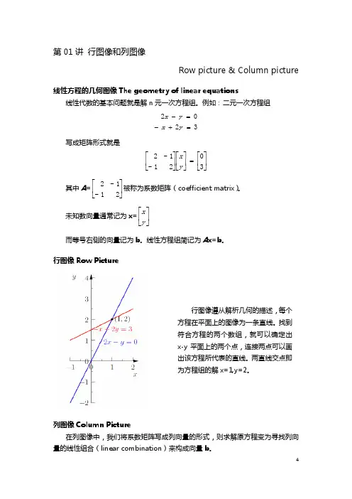
Chapter 1 Matrices and Systems of EquationsLinear systems arise in applications to such areas as engineering, physics, electronics, business, economics, sociology(社会学), ecology (生态学), demography(人口统计学), and genetics(遗传学), etc. §1. Systems of Linear EquationsNew words and phrases in this section:Linear equation 线性方程Linear system,System of linear equations 线性方程组Unknown 未知量Consistent 相容的Consistence 相容性Inconsistent不相容的Inconsistence 不相容性Solution 解Solution set 解集Equivalent 等价的Equivalence 等价性Equivalent system 等价方程组Strict triangular system 严格上三角方程组Strict triangular form 严格上三角形式Back Substitution 回代法Matrix 矩阵Coefficient matrix 系数矩阵Augmented matrix 增广矩阵Pivot element 主元Pivotal row 主行Echelon form 阶梯形1.1 DefinitionsA linear equation (线性方程) in n unknowns(未知量)is1122...n na x a x a x b+++=A linear system of m equations in n unknowns is11112211211222221122...... .........n n n n m m m n n m a x a x a x b a x a x a x b a x a x a x b+++=⎧⎪+++=⎪⎨⎪⎪+++=⎩ This is called a m x n (read as m by n) system.A solution to an m x n system is an ordered n-tuple of numbers (n 元数组)12(,,...,)n x x x that satisfies all the equations.A system is said to be inconsistent (不相容的) if the system has no solutions.A system is said to be consistent (相容的)if the system has at least one solution.The set of all solutions to a linear system is called the solution set(解集)of the linear system.1.2 Geometric Interpretations of 2x2 Systems11112212112222a x a xb a x a x b +=⎧⎨+=⎩ Each equation can be represented graphically as a line in the plane. The ordered pair 12(,)x x will be a solution if and only if it lies on bothlines.In the plane, the possible relative positions are(1) two lines intersect at exactly a point; (The solution set has exactly one element)(2)two lines are parallel; (The solution set is empty)(3)two lines coincide. (The solution set has infinitely manyelements)The situation is the same for mxn systems. An mxn system may not be consistent. If it is consistent, it must either have exactly one solution or infinitely many solutions. These are only possibilities.Of more immediate concerns is the problem of finding all solutions to a given system.1.3 Equivalent systemsTwo systems of equations involving the same variables are said to be equivalent(等价的,同解的)if they have the same solution set.To find the solution set of a system, we usually use operations to reduce the original system to a simpler equivalent system.It is clear that the following three operations do not change the solution set of a system.(1)Interchange the order in which two equations of a system arewritten;(2)Multiply through one equation of a system by a nonzero realnumber;(3)Add a multiple of one equation to another equation. (subtracta multiple of one equation from another one)Remark: The three operations above are very important in dealing with linear systems. They coincide with the three row operations of matrices. Ask a student about the proof.1.4 n x n systemsIf an nxn system has exactly one solution, then operation 1 and 3 can be used to obtain an equivalent “strictly triangular system ”A system is said to be in strict triangular form (严格三角形) if in the k-th equation the coefficients of the first k-1 variables are all zero and the coefficient ofkx is nonzero. (k=1, 2, …,n)An example of a system in strict triangular form:123233331 2 24x x x x x x ++=⎧⎪-=⎨⎪=⎩Any nxn strictly triangular system can be solved by back substitution (回代法).(Note: A phrase: “substitute 3 for x ” == “replace x by 3”)In general, given a system of linear equations in n unknowns, we will use operation I and III to try to obtain an equivalent system that is strictly triangular.We can associate with a linear system an mxn array of numbers whose entries are coefficient of theix ’s. we will refer to this array as thecoefficient matrix (系数矩阵) of the system.111212122212.....................n nm m m n a a a a a a a a a ⎛⎫⎪ ⎪ ⎪ ⎪⎝⎭A matrix (矩阵) is a rectangular array of numbersIf we attach to the coefficient matrix an additional column whose entries are the numbers on the right-hand side of the system, we obtain the new matrix11121121222212n n s m m m na a ab a a a b b a a a ⎛⎫ ⎪ ⎪ ⎪⎝⎭We refer to this new matrix as the augmented matrix (增广矩阵) of a linear system.The system can be solved by performing operations on the augmented matrix. i x ’s are placeholders that can be omitted until the endof computation.Corresponding to the three operations used to obtain equivalent systems, the following row operation may be applied to the augmented matrix.1.5 Elementary row operationsThere are three elementary row operations:(1)Interchange two rows;(2)Multiply a row by a nonzero number;(3)Replace a row by its sum with a multiple of another row.Remark: The importance of these three operations is that they do not change the solution set of a linear system and may reduce a linear system to a simpler form.An example is given here to illustrate how to perform row operations on a matrix.★Example:The procedure for applying the three elementary row operations:Step 1: Choose a pivot element (主元)(nonzero) from among the entries in the first column. The row containing the pivotnumber is called a pivotal row(主行). We interchange therows (if necessary) so that the pivotal row is the new firstrow.Multiples of the pivotal row are then subtracted form each of the remaining n-1 rows so as to obtain 0’s in the firstentries of rows 2 through n.Step2: Choose a pivot element from the nonzero entries in column 2, rows 2 through n of the matrix. The row containing thepivot element is then interchanged with the second row ( ifnecessary) of the matrix and is used as the new pivotal row.Multiples of the pivotal row are then subtracted form eachof the remaining n-2 rows so as to eliminate all entries belowthe pivot element in the second column.Step 3: The same procedure is repeated for columns 3 through n-1.Note that at the second step, row 1 and column 1 remain unchanged, at the third step, the first two rows and first two columns remain unchanged, and so on.At each step, the overall dimensions of the system are effectively reduced by 1. (The number of equations and the number of unknowns all decrease by 1.)If the elimination process can be carried out as described, we will arrive at an equivalent strictly triangular system after n-1 steps.However, the procedure will break down if all possible choices for a pivot element are all zero. When this happens, the alternative is to reduce the system to certain special echelon form(梯形矩阵). AssignmentStudents should be able to do all problems.Hand-in problems are: # 7--#11§2. Row Echelon FormNew words and phrases:Row echelon form 行阶梯形Reduced echelon form 简化阶梯形 Lead variable 首变量 Free variable 自由变量Gaussian elimination 高斯消元Gaussian-Jordan reduction. 高斯-若当消元 Overdetermined system 超定方程组 Underdetermined systemHomogeneous system 齐次方程组 Trivial solution 平凡解2.1 Examples and DefinitionIn this section, we discuss how to use elementary row operations to solve mxn systems.Use an example to illustrate the idea.★ Example : Example 1 on page 13. Consider a system represented by the augmented matrix111111110011220031001131112241⎛⎫ ⎪--- ⎪ ⎪-- ⎪- ⎪ ⎪⎝⎭ 111111001120002253001131001130⎛⎫⎪ ⎪ ⎪ ⎪- ⎪ ⎪⎝⎭………..(The details will given in class)We see that at this stage the reduction to strict triangular form breaks down. Since our goal is to simplify the system as much as possible, we move over to the third column. From the example above, we see that the coefficient matrix that we end up with is not in strict triangular form,it is in staircase or echelon form (梯形矩阵).111111001120000013000004003⎛⎫ ⎪ ⎪ ⎪ ⎪- ⎪ ⎪-⎝⎭The equations represented by the last two rows are:12345345512=0 2=3 0=4 03x x x x x x x x x ++++=⎧⎪++⎪⎪⎨⎪-⎪=-⎪⎩Since there are no 5-tuples that could possibly satisfy these equations, the system is inconsistent.Change the system above to a consistent system.111111110011220031001133112244⎛⎫ ⎪--- ⎪ ⎪-- ⎪ ⎪ ⎪⎝⎭ 111111001120000013000000000⎛⎫⎪ ⎪ ⎪ ⎪ ⎪ ⎪⎝⎭The last two equations of the reduced system will be satisfied for any 5-tuple. Thus the solution set will be the set of all 5-tuples satisfying the first 3 equations.The variables corresponding to the first nonzero element in each row of the augment matrix will be referred to as lead variable .(首变量) The remaining variables corresponding to the columns skipped in the reduction process will be referred to as free variables (自由变量).If we transfer the free variables over to the right-hand side in the above system, then we obtain the system:1352435451 2 3x x x x x x x x x ++=--⎧⎪+=-⎨⎪=⎩which is strictly triangular in the unknown 1x 3x 5x . Thus for each pairof values assigned to 2xand4x , there will be a unique solution.★Definition: A matrix is said to be in row echelon form (i) If the first nonzero entry in each nonzero row is 1.(ii)If row k does not consist entirely of zeros, the number of leading zero entries in row k+1 is greater than the number of leading zero entries in row k.(iii) If there are rows whose entries are all zero, they are below therows having nonzero entries.★Definition : The process of using row operations I, II and III to transform a linear system into one whose augmented matrix is in row echelon form is called Gaussian elimination (高斯消元法).Note that row operation II is necessary in order to scale the rows so that the lead coefficients are all 1.It is clear that if the row echelon form of the augmented matrix contains a row of the form (), the system is inconsistent.000|1Otherwise, the system will be consistent.If the system is consistent and the nonzero rows of the row echelon form of the matrix form a strictly triangular system (the number of nonzero rows<the number of unknowns), the system will have a unique solution. If the number of nonzero rows<the number of unknowns, then the system has infinitely many solutions. (There must be at least one free variable. We can assign the free variables arbitrary values and solve for the lead variables.)2.2 Overdetermined SystemsA linear system is said to be overdetermined if there are more equations than unknowns.2.3 Underdetermined SystemsA system of m linear equations in n unknowns is said to be underdetermined if there are fewer equations than unknowns (m<n). It is impossible for an underdetermined system to have only one solution.In the case where the row echelon form of a consistent system has free variables, it is convenient to continue the elimination process until all the entries above each lead 1 have been eliminated. The resulting reduced matrix is said to be in reduced row echelon form. For instance,111111001120000013000000000⎛⎫ ⎪ ⎪ ⎪ ⎪ ⎪ ⎪⎝⎭ 110004001106000013000000000⎛⎫⎪- ⎪ ⎪ ⎪ ⎪ ⎪⎝⎭Put the free variables on the right-hand side, it follows that12345463x x x x x =-=--=Thus for any real numbersαandβ, the 5-tuple()463ααββ---is a solution.Thus all ordered 5-tuple of the form ()463ααββ--- aresolutions to the system.2.4 Reduced Row Echelon Form★Definition : A matrix is said to be in reduced row echelon form if :(i)the matrix is in row echelon form.(ii) The first nonzero entry in each row is the only nonzero entry in its column.The process of using elementary row operations to transform a matrix into reduced echelon form is called Gaussian-Jordan reduction.The procedure for solving a linear system:(i) Write down the augmented matrix associated to the system; (ii) Perform elementary row operations to reduce the augmented matrix into a row echelon form;(iii) If the system if consistent, reduce the row echelon form into areduced row echelon form. (iv) Write the solution in an n-tuple formRemark: Make sure that the students know the difference between the row echelon form and the reduced echelon form.Example 6 on page 18: Use Gauss-Jordan reduction to solve the system:1234123412343030220x x x x x x x x x x x x -+-+=⎧⎪+--=⎨⎪---=⎩The details of the solution will be given in class.2.5 Homogeneous SystemsA system of linear equations is said to be homogeneous if theconstants on the right-hand side are all zero.Homogeneous systems are always consistent since it has a trivial solution. If a homogeneous system has a unique solution, it must be the trivial solution.In the case that m<n (an underdetermined system), there will always free variables and, consequently, additional nontrivial solution.Theorem 1.2.1 An mxn homogeneous system of linear equations has a nontrivial solution if m<n.Proof A homogeneous system is always consistent. The row echelon form of the augmented matrix can have at most m nonzero rows. Thus there are at most m lead variables. There must be some free variable. The free variables can be assigned arbitrary values. For each assignment of values to the free variables, there is a solution to the system.AssignmentStudents should be able to do all problems except 17, 18, 20.Hand-in problems are 9, 10, 16,Select one problem from 14 and 19.§3. Matrix AlgebraNew words and phrases:Algebra 代数Scalar 数量,标量Scalar multiplication 数乘 Real number 实数 Complex number 复数 V ector 向量Row vector 行向量 Column vector 列向量Euclidean n-space n 维欧氏空间 Linear combination 线性组合 Zero matrix 零矩阵Identity matrix 单位矩阵 Diagonal matrix 对角矩阵 Triangular matrix 三角矩阵Upper triangular matrix 上三角矩阵 Lower triangular matrix 下三角矩阵 Transpose of a matrix 矩阵的转置(Multiplicative ) Inverse of a matrix 矩阵的逆 Singular matrix 奇异矩阵 Singularity 奇异性Nonsingular matrix 非奇异矩阵 Nonsingularity 非奇异性The term scalar (标量,数量) is referred to as a real number (实数) or a complex number (复数). Matrix notationAn mxn matrix, a rectangular array of mn numbers.111212122212.....................n nm m m n a a a a a a a a a ⎛⎫⎪ ⎪ ⎪ ⎪⎝⎭()ij A a =3.1 VectorsMatrices that have only one row or one column are of special interest since they are used to represent solutions to linear systems.We will refer to an ordered n-tuple of real numbers as a vector (向量).If an n-tuple is represented in terms of a 1xn matrix, then we will refer to it as a row vector . Alternatively, if the n-tuple is represented by an nx1 matrix, then we will refer to it as a column vector . In this course, we represent a vector as a column vector.The set of all nx1 matrices of real number is called Euclidean n-space (n 维欧氏空间) and is usually denoted by nR.Given a mxn matrix A, it is often necessary to refer to a particular row or column. The matrix A can be represented in terms of either its column vectors or its row vectors.12(a ,a ,,a )n A = ora (1,:)a(2,:)a(,:)A m ⎛⎫ ⎪⎪= ⎪ ⎪⎝⎭3.2 EqualityFor two matrices to be equal, they must have the same dimensions and their corresponding entries must agree★Definition : Two mxn matrices A and B are said to be equal ifij ij a b =for each ordered pair (i, j)3.3 Scalar MultiplicationIf A is a matrix,αis a scalar, thenαA is the mxn matrix formed by multiplying each of the entries of A byα.★Definition : If A is an mxn matrix, αis a scalar, thenαA is themxn matrix whose (i, j) is ij a αfor each ordered pair (i, j) .3.4 Matrix AdditionTwo matrices with the same dimensions can be added by adding their corresponding entries.★Definition : If A and B are both mxn matrices, then the sum A+B is the mxn matrix whose (i,j) entry isij ija b + for each ordered pair (i, j).An mxn zero matrix (零矩阵) is a matrix whose entries are all zero. It acts as an additive identity on the set of all mxn matrices.A+O=O+A=AThe additive of A is (-1)A since A+(-1)A=O=(-1)A+A.A-B=A+(-1)B-A=(-1)A3.5 Matrix Multiplication and Linear Systems3.5.1 MotivationsRepresent a linear system as a matrix equationWe have yet to defined the most important operation, the multiplications of two matrices. A 1x1 system can be writtena xb =A scalar can be treated as a 1x1 matrix. Our goal is to generalize the equation above so that we can represent an mxn system by a single equation.A X B=Case 1: 1xn systems 1122... n n a x a x a x b +++=If we set()12n A a a a =and12n x x X x ⎛⎫ ⎪⎪= ⎪ ⎪⎝⎭, and define1122...n n AX a x a x a x =+++Then the equation can be written as A X b =。
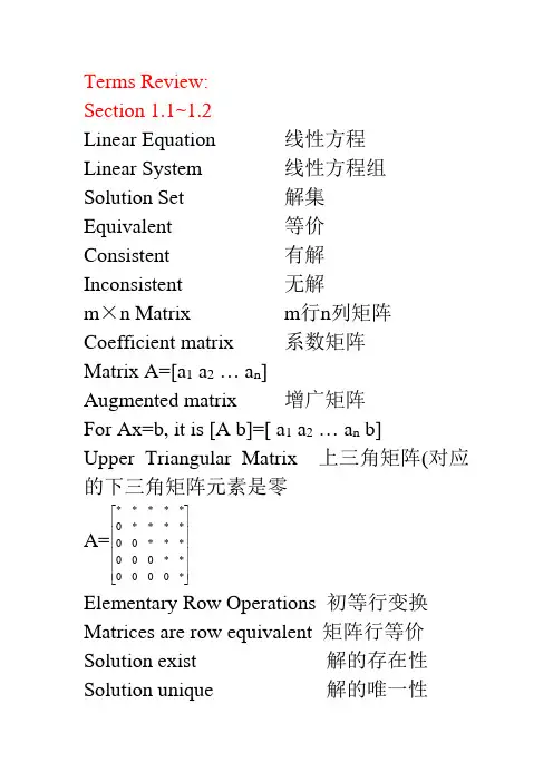
Terms Review: Section 1.1~1.2 Linear Equation 线性方程 Linear System 线性方程组 Solution Set 解集 Equivalent 等价 Consistent 有解 Inconsistent 无解 m ×n Matrix m 行n 列矩阵 Coefficient matrix 系数矩阵 Matrix A=[a 1 a 2 … a n ] Augmented matrix 增广矩阵 For Ax=b, it is [A b]=[ a 1 a 2 … a n b]Upper Triangular Matrix 上三角矩阵(对应的下三角矩阵元素是零 A=⎥⎥⎥⎥⎥⎥⎦⎤⎢⎢⎢⎢⎢⎢⎣⎡*0000**000***00****0*****Elementary Row Operations 初等行变换 Matrices are row equivalent 矩阵行等价 Solution exist 解的存在性 Solution unique 解的唯一性Leading entry 前导项,左端第一个非零项Echelon Matrix 阶梯矩阵Reduced echelon form 简化的阶梯形式Pivot position 主元位置Pivot column 主元列Basic variable 基变量Free variable 自由变量General solution 通解Home Work Due on March 4:Section 1.1Practice Problem 2Exercises16, 18, 23, 24Section 1.2Practice Problem 14, 14, 21, 24Section 1.123.a.True or T. See the remarks following thebox titled “Elementary Row Operations”b.False or F. The size of a matrix is definedjust before the subsection titled “Solving a Linear System.”c.F. The solution set of a linear system is theset of all solutions of the system. See page 3d.T. See the box before Example2.24.a.T. See the grayed statement on page 8.b.F. The definition is given on page 7,or just by definition.c.F. The definition is given on page 4.d.T. The definition is given on page 5.Section 1.3~1.5Column vector 列向量Scalar multiple 标量数乘Linear combination 线性组合Weights 权重Span{v1,…,v p}-subset of R n spanned by v1,…,v p由向量v1,…,v p生成的n维欧氏空间的子集Span = generate 张成,生成The columns of A span R m矩阵A的列向量张成R mHomogeneous 齐次Trivial solution 零解,平凡解Nontrivial trivial solution 非零解,非平凡解Parametric vector equation 带参数的向量方程Home Work Due on March 11:Section 1.36,10, 12, 18,23, 24Section 1.422, 23,24,26, 32Section 1.6~1.7Linear independent 线性无关Linear dependent 线性相关Linear Transformation 线性变换Mapping 映射Domain 域Codomain 上域Image 像Range 值域Matrix Transformation 矩阵变换Shear 剪切Superposition principle 叠加原理Contraction 压缩Dilation 膨胀Section 1.8Identity Matrix In 单位矩阵In=⎥⎥⎥⎦⎤⎢⎢⎢⎣⎡111Standard Matrix for the linear transformationT线性变换T 的标准矩阵 Reflection 反射 Onto Mapping 到上映射 One-to-One Mapping 一一映射Section 1.6Thm8If a set contains more vectors than there are entries in each vector, then the set is linearlydependent. I.e. any set {v 1,v 2,…,v p } in R nis linearly dependent if p>n.Proof:Let A=[v 1,…,v p ], then A is n ×p, and Ax=0 corresponds to a system of n equations in punkowns. If p>n, there are more variables than equations, so there must be a free variable. Hence Ax=0 has a nontrivial solution and the columns of A are linearly dependent.For exampleA= [ a 1 a 2 a 3 a 4 a 5]=⎥⎥⎥⎦⎤⎢⎢⎢⎣⎡***************, {a 1,…,a 5} aredependent. But columns of Matrix with 5×3 areunknown.Thm7 Proof:(1) If some v j in S equals a linear combinationof the other vectors, then v j can be subtracted from both sides of the equation, producing a linear dependence relation with a nonzero weight (-1) on v j . For instance, if v 1=c 2v 2+c 3v 3, then0=(-1)v 1+c 2v 2+c 3v 3+0v 4+…+0v p Thus S in linearly dependent.(2) Conversely, suppose S is linearly dependent,If v 1 is zero, then it is a trivial linear combination of other vectors in S. Otherwise, v 1≠0 and there exist weights c 1,…,c p , not all zero, such that c 1v 1+c 2v 2+…+c p v p =0, let j be the largest subscript for which c j ≠0, If j=1, then c 1v 1=0, which is impossible because v 1≠0, so j>1 andc 1v 1+…+c j v j +0v j+1+…+0v p =0, c j v j =-c 1v 1-…-c j-1v j-1,v j =(-c 1/c j )v 1+…+(-c j-1/c j )v j-1█Section 1.8 Thm10 Proof:The existence of A:Write x=I n x=[e 1 … e n ]x=x 1e 1+…+x n e n , and use the linearity of T to computeT(x)=T(x 1e 1+…+x n e n )= x 1T(e 1)+…+x n T(e n ) =[ T(e 1) …T(e n )]⎥⎥⎥⎦⎤⎢⎢⎢⎣⎡n x x 1=AxThe uniqueness of A:Define T: R n→R m by T(x)=Bx for some m×n matrix B, and let A be the standard matrix for T. By definition, A=[ T(e1) …T(e n)], where e j is the jth column of I n. However, by matrix-vector multiplication, T(e j)=B e j = b j , the jth column of B. So A=[ b1… b n]=B.█Every linear transformation from R n to R m is a matrix transformation and vice versa. (p77) Every matrix transformation is a linear transformation. Examples of linear transformations that are not matrix transformation will be discussed in Chapters 4 and 5. (p70)Refer to p244, Theorem 8Let B={b1,…,b n} be a basis for a vector space V. Then the coordinate mapping x|→[x]B is a one-to-one linear transformation from V onto R n.Example 5+=p(t)=a0+a1t+a2t2+a3t3[x]B =[p]B =(a 0,a 1,a 2,a 3)This example is linear transformation, but not matrix transformation.So answer for Exercise 24(a) is False.Example 3Let T:R 2→R 2be the transformation that rotateseach point in R 2through an angle φ, with counterclockwise rotation for a positive angle. Find the standard matrix A of this transformation. Sol:⎥⎦⎤⎢⎣⎡01 rotates into ⎥⎦⎤⎢⎣⎡ϕϕsin cos ,⎥⎦⎤⎢⎣⎡10 rotates into⎥⎦⎤⎢⎣⎡-ϕϕcos sin .By Thm10⎥⎦⎤⎢⎣⎡-=ϕϕϕϕcos sin sin cos AGeometric Linear Transformation of R2 1. ReflectionsStandard matrix a. in x 1-axis ⎥⎦⎤⎢⎣⎡-1001b. in x 2-axis ⎥⎦⎤⎢⎣⎡-1001 c. in line x 2=-x 1 ⎥⎦⎤⎢⎣⎡--0110 d. in line x 2=x1 ⎥⎦⎤⎢⎣⎡0110 e. in origin⎥⎦⎤⎢⎣⎡--10012. Contractions (k<1) and Expansions (k>1) a. Horizontal ⎥⎦⎤⎢⎣⎡100k b. Vertical ⎥⎦⎤⎢⎣⎡k 0013. Shearsa. Horizontal ⎥⎦⎤⎢⎣⎡101kb. Vertical ⎥⎦⎤⎢⎣⎡101k4. Projection a. Onto x1-axis ⎥⎦⎤⎢⎣⎡0001 b. Onto x2-axis⎥⎦⎤⎢⎣⎡1000Existence and Uniqueness Questions.Def. A mapping T: R n →R m is said to be onto R mif each b in R mis the image of at least one x in R n .Equivalently, T is onto R m if for each b in R mthere exists at least one solution of T(x)=b.“Does T map R n onto R m?” is an existence question. T is not onto when there is some b in R m such that the equation T(x)=b has no solution.Def. A mapping T: R n →R m is said to beone-to-one (or 1:1) if each b in R mis the imageof at most one x in R n.Equivalently, T is 1:1 if for each b in R mthere exists a unique or none solution of T(x)=b. “Is T one-to-one?” is a uniqueness question. T is not1:1 when some b in R mis the image of more than one vector in R n .Example 4 T(x)=Ax=⎥⎥⎥⎦⎤⎢⎢⎢⎣⎡--500031201841x, Does T map R4onto R 3? Is T a 1:1 mapping?Sol:A has a pivot position in each row, by Thm4 in Seciton1.4, for each b in R 3 , Ax=b is consistent.So T map R 4 onto R 3.However, since the equation Ax=b has a free variable, each b is the image of more than one x. So, T is not 1:1.Thm11.Let T: R n→R m be a linear transformation, then T is 1:1 iff T(x)=0 has only the trivial solution. Proof:(1)If T is 1:1, then T(x)=0 has at most onesolution and hence only the trivialsolution.(2)If T(x)=0 has only the trivial solution, it isfalse to say T is not 1:1. Otherwise, thereis a b that is the image of at least twodifferent vectors in R n , say, u and v, u≠v,T(u)=T(v)=b. Since T is linear,T(u-v)=T(u)-T(v)=0, but u-v≠0. HenceT(x)=0 has more than one solution.Contradiction. So T is 1:1.█Thm12Let T: R n→R m be a linear transformation, and letA be the standard matrix for T, then:(a). T maps R n onto R m iff the columns of A span R m .(b). T is 1:1 iff the columns of A are linearly independent.Proof:(a). By thm4 in section1.4, the columns of A span R m iff for each b, Ax=b is consistent, i.e., iff for every b, T(x)=b has at least one solution. This is true iff T maps R n onto R m(b). T(x)=0 and Ax=0 are the same except for notation. So by Thm11, T is 1:1 iff Ax=0 has only the trivial solution. This happens iff the columns of A are linearly independent, as was already noted in the boxed statement (3) in section 1.6.█Example 5Let T(x1,x2)=(3x1+x2, 5x1+7x2, x1+3x2). Does T map R2onto R3? Is T 1:1?Sol:T(x)=Ax=⎥⎦⎤⎢⎣⎡⎥⎥⎥⎦⎤⎢⎢⎢⎣⎡x xx 1371153, since columns of A arelinearly independent, by Thm12(b), T is 1:1.Since A is 3×2, the columns of A span R 3 iff A has 3 pivot position, by Thm4. This is impossible. Since A has only 2 columns. So T is not onto R 3Home Work Due on March 16: Section 1.512, 21, 22, 25,32 Section 1.618,30,32,34,36,39Home Work Due on March 23: Section 1.74,12,23,24,26,34Section 1.86,8,10,23, 24Definitions:1.The definition of Ax in both words and symbols.2.Span { v } , Span { u; v } and geometric interpretation in R2 or R3 .3.Span { v1,…, v p } .4.Linearly independent and linearly dependent.5.Linear transformation.Chapter 1 Theorems:1.Theorem 2 (Existence and Uniqueness Theorem).2.Theorem 3 (Matrix equation, vector equation, system of linear equations).3.Theorem 4 (When do the columns of A span R m ?).4.Theorem 5 (Properties of the Matrix-Vector Product Ax).5.Theorems 6, 7, 8 (Properties of linearly dependent sets).Important Skills1.Determine when a system is consistent. Write the general solution in parametric vector form as a linear combination of vectors using the free variables as parameters.2.Determine values of parameters that make a system consistent, or make the solution unique.3.Describe existence or uniqueness of solutions in terms of pivot positions. Determine when a homogeneous system hasa nontrivial solution.4.Determine when a vector is in a subset spanned by specified vectors. Exhibit a vector as a linear combination of specified vectors.5.Determine whether the columns of an m _ n matrix span R m .e linearity of matrix multiplication to compute A(u + v) or A(cu).7.Determine when a set of vectors is linearlyindependent. Know several methods that can sometimes produce an answer “by inspection” (without much calculation).。
4 LINEAR ALGEBRA 线性代数“Linear algebra” is the study of linear sets of equations and their transformation properties. 线性代数是研究方程的线性几何以及他们的变换性质的Linear algebra allows the analysis of rotations in space, least squares fitting, solution of coupled differential equations, determination of a circle passing through three given points, as well as many other problems in mathematics, physics, and engineering.线性代数也研究空间旋转的分析,最小二乘拟合,耦合微分方程的解,确立通过三个已知点的一个圆以及在数学、物理和机械工程上的其他问题The matrix and determinant are extremely useful tools of linear algebra.矩阵和行列式是线性代数极为有用的工具One central problem of linear algebra is the solution of the matrix equation Ax = b for x. 线性代数的一个中心问题是矩阵方程Ax=b关于x的解While this can, in theory, be solved using a matrix inverse x = A−1b,other techniques such as Gaussian elimination are numerically more robust.理论上,他们可以用矩阵的逆x=A-1b求解,其他的做法例如高斯消去法在数值上更鲁棒。
线性代数英语词汇大集合========================================================================= Aadjont(adjugate) of matrix A A 的伴随矩阵augmented matrix A 的增广矩阵Bblock diagonal matrix 块对角矩阵block matrix 块矩阵basic solution set 基础解系CCauchy-Schwarz inequality 柯西- 许瓦兹不等式characteristic equation 特征方程characteristic polynomial 特征多项式coffcient matrix 系数矩阵cofactor 代数余子式cofactor expansion 代数余子式展开column vector 列向量commuting matrices 交换矩阵consistent linear system 相容线性方程组Cramer's rule 克莱姆法则Cross- product term 交叉项DDeterminant 行列式Diagonal entries 对角元素Diagonal matrix 对角矩阵Dimension of a vector space V 向量空间V 的维数Eechelon matrix 梯形矩阵eigenspace 特征空间eigenvalue 特征值eigenvector 特征向量eigenvector basis 特征向量的基elementary matrix 初等矩阵elementary row operations 行初等变换Ffull rank 满秩fundermental set of solution 基础解系Ggrneral solution 通解Gram-Schmidt process 施密特正交化过程Hhomogeneous linear equations 齐次线性方程组Iidentity matrix 单位矩阵inconsistent linear system 不相容线性方程组indefinite matrix 不定矩阵indefinit quatratic form 不定二次型infinite-dimensional space 无限维空间inner product 内积inverse of matrix A 逆矩阵JKLlinear combination 线性组合linearly dependent 线性相关linearly independent 线性无关linear transformation 线性变换lower triangular matrix 下三角形矩阵Mmain diagonal of matrix A 矩阵的主对角matrix 矩阵Nnegative definite quaratic form 负定二次型negative semidefinite quadratic form 半负定二次型nonhomogeneous equations 非齐次线性方程组nonsigular matrix 非奇异矩阵nontrivial solution 非平凡解norm of vector V 向量V 的范数normalizing vector V 规范化向量Oorthogonal basis 正交基orthogonal complemen t 正交补orthogonal decomposition 正交分解orthogonally diagonalizable matrix 矩阵的正交对角化orthogonal matrix 正交矩阵orthogonal set 正交向量组orthonormal basis 规范正交基orthonomal set 规范正交向量组Ppartitioned matrix 分块矩阵positive definite matrix 正定矩阵positive definite quatratic form 正定二次型positive semidefinite matrix 半正定矩阵positive semidefinite quadratic form 半正定二次型Qquatratic form 二次型Rrank of matrix A 矩阵A 的秩r(A )reduced echelon matrix 最简梯形阵row vector 行向量Sset spanned by { } 由向量{ } 所生成similar matrices 相似矩阵similarity transformation 相似变换singular matrix 奇异矩阵solution set 解集合standard basis 标准基standard matrix 标准矩阵Isubmatrix 子矩阵subspace 子空间symmetric matrix 对称矩阵Ttrace of matrix A 矩阵A 的迹tr ( A )transpose of A 矩阵A 的转秩triangle inequlity 三角不等式trivial solution 平凡解Uunit vector 单位向量upper triangular matrix 上三角形矩阵Vvandermonde matrix 范得蒙矩阵vector 向量vector space 向量空间WZzero subspace 零子空间zero vector 零空间==============================================================================向量:vector 向量的长度(模):零向量: zero vector负向量: 向量的加法:addition 三角形法则:平行四边形法则:多边形法则减法向量的标量乘积:scalar multiplication 向量的线性运算线性组合:linear combination 线性表示,线性相关(linearly dependent),线性无关(linearly independent),原点(origin)位置向量(position vector)线性流形(linear manifold)线性子空间(linear subspace)基(basis)仿射坐标(affine coordinates),仿射标架(affine frame),仿射坐标系(affine coordinate system)坐标轴(coordinate axis)坐标平面卦限(octant)右手系左手系定比分点线性方程组(system of linear equations齐次线性方程组(system of homogeneous linear equations)行列式(determinant)维向量向量的分量(component)向量的相等和向量零向量负向量标量乘积维向量空间(vector space)自然基行向量(row vector)列向量(column vector)单位向量(unit vector)直角坐标系(rectangular coordinate system),直角坐标(rectangular coordinates),射影(projection)向量在某方向上的分量,正交分解,向量的夹角,内积(inner product)标量积(scalar product),数量积,方向的方向角,方向的方向余弦;二重外积外积(exterior product),向量积(cross product),混合积(mixed product,scalar triple product)==================================================================================(映射(mapping)),(象(image)),(一个原象(preimage)),(定义域(domain)),(值域(range)),(变换(transformation)),(单射(injection)),(象集),(满射(surjection)),(一一映射,双射(bijection)),(原象),(映射的复合,映射的乘积),(恒同映射,恒同变换(identity mapping)),(逆映射(inverse mapping));(置换(permutation)),(阶对称群(symmetric group)),(对换(transposition)),(逆序对),(逆序数),(置换的符号(sign)),(偶置换(even permutation)),(奇置换(odd permutation));行列式(determinant),矩阵(matrix),矩阵的元(entry),(方阵(square matrix)),(零矩阵(zero matrix)),(对角元),(上三角形矩阵(upper triangular matrix)),(下三角形矩阵(lower triangular matrix)),(对角矩阵(diagonal matrix)),(单位矩阵(identity matrix)),转置矩阵(transpose matrix),初等行变换(elementary row transformation),初等列变换(elementary column transformation);(反称矩阵(skew-symmetric matrix));子矩阵(submatrix),子式(minor),余子式(cofactor),代数余子式(algebraic cofactor),(范德蒙德行列式(Vandermonde determinant));(未知量),(系数矩阵),(方程的系数(coefficient)),(常数项(constant)),(线性方程组的解(solution)),(增广矩阵(augmented matrix)),(零解);子式的余子式,子式的代数余子式===================================================================================线性方程组与线性子空间(阶梯形方程组),(方程组的初等变换),行阶梯矩阵(row echelon matrix),主元,简化行阶梯矩阵(reduced row echelon matrix),(高斯消元法(Gauss elimination)),(解向量),(同解),(自反性(reflexivity)),(对称性(symmetry)),(传递性(transitivity)),(等价关系(equivalence));(齐次线性方程组的秩(rank));(主变量),(自由位置量),(一般解),向量组线性相关,向量组线性无关,线性组合,线性表示,线性组合的系数,(向量组的延伸组);线性子空间,由向量组张成的线性子空间;基,坐标,(自然基),向量组的秩;(解空间),线性子空间的维数(dimension),齐次线性方程组的基础解系(fundamental system of solutions);(平面束(pencil of planes))(导出组),线性流形,(方向子空间),(线性流形的维数),(方程组的特解);(方程组的零点),(方程组的图象),(平面的一般方程),(平面的三点式方程),(平面的截距式方程),(平面的参数方程),(参数),(方向向量);(直线的方向向量),(直线的参数方程),(直线的标准方程),(直线的方向系数),(直线的两点式方程),(直线的一般方程);=====================================================================================矩阵的秩与矩阵的运算线性表示,线性等价,极大线性无关组;(行空间,列空间),行秩(row rank),列秩(column rank),秩,满秩矩阵,行满秩矩阵,列满秩矩阵;线性映射(linear mapping),线性变换(linear transformation),线性函数(linear function);(零映射),(负映射),(矩阵的和),(负矩阵),(线性映射的标量乘积),(矩阵的标量乘积),(矩阵的乘积),(零因子),(标量矩阵(scalar matrix)),(矩阵的多项式);(退化的(degenerate)方阵),(非退化的(non-degenerate)方阵),(退化的线性变换),(非退化的线性变换),(逆矩阵(inverse matrix)),(可逆的(invertible),(伴随矩阵(adjoint matrix));(分块矩阵(block matrix)),(分块对角矩阵(block diagonal matrix));初等矩阵(elementary matrix),等价(equivalent);(象空间),(核空间(kernel)),(线性映射的秩),(零化度(nullity))==================================================================================== transpose of matrix 倒置矩阵; 转置矩阵【数学词汇】transposed matrix 转置矩阵【机械专业词汇】matrix transpose 矩阵转置【主科技词汇】transposed inverse matrix 转置逆矩阵【数学词汇】transpose of a matrix 矩阵的转置【主科技词汇】permutation matrix 置换矩阵; 排列矩阵【主科技词汇】singular matrix 奇异矩阵; 退化矩阵; 降秩矩阵【主科技词汇】unitary matrix 单式矩阵; 酉矩阵; 幺正矩阵【主科技词汇】Hermitian matrix 厄密矩阵; 埃尔米特矩阵; 艾米矩阵【主科技词汇】inverse matrix 逆矩阵; 反矩阵; 反行列式; 矩阵反演; 矩阵求逆【主科技词汇】matrix notation 矩阵符号; 矩阵符号表示; 矩阵记号; 矩阵运算【主科技词汇】state transition matrix 状态转变矩阵; 状态转移矩阵【航海航天词汇】torque master 转矩传感器; 转矩检测装置【主科技词汇】spin matrix 自旋矩阵; 旋转矩阵【主科技词汇】moment matrix 动差矩阵; 矩量矩阵【航海航天词汇】Jacobian matrix 雅可比矩阵; 导数矩阵【主科技词汇】relay matrix 继电器矩阵; 插接矩阵【主科技词汇】matrix notation 矩阵表示法; 矩阵符号【航海航天词汇】permutation matrix 置换矩阵【航海航天词汇】transition matrix 转移矩阵【数学词汇】transition matrix 转移矩阵【机械专业词汇】transitionmatrix 转移矩阵【航海航天词汇】transition matrix 转移矩阵【计算机网络词汇】transfer matrix 转移矩阵【物理词汇】rotation matrix 旋转矩阵【石油词汇】transition matrix 转换矩阵【主科技词汇】circulant matrix 循环矩阵; 轮换矩阵【主科技词汇】payoff matrix 报偿矩阵; 支付矩阵【主科技词汇】switching matrix 开关矩阵; 切换矩阵【主科技词汇】method of transition matrices 转换矩阵法【航海航天词汇】stalling torque 堵转力矩, 颠覆力矩, 停转转矩, 逆转转矩【航海航天词汇】thin-film switching matrix 薄膜转换矩阵【航海航天词汇】rotated factor matrix 旋转因子矩阵【航海航天词汇】transfer function matrix 转移函数矩阵【航海航天词汇】transition probability matrix 转移概率矩阵【主科技词汇】energy transfer matrix 能量转移矩阵【主科技词汇】fuzzy transition matrix 模糊转移矩阵【主科技词汇】canonical transition matrix 规范转移矩阵【主科技词汇】matrix form 矩阵式; 矩阵组织【主科技词汇】stochastic state transition matrix 随机状态转移矩阵【主科技词汇】fuzzy state transition matrix 模糊状态转移矩阵【主科技词汇】matrix compiler 矩阵编码器; 矩阵编译程序【主科技词汇】test matrix 试验矩阵; 测试矩阵; 检验矩阵【主科技词汇】matrix circuit 矩阵变换电路; 矩阵线路【主科技词汇】reducible matrix 可简化的矩阵; 可约矩阵【主科技词汇】matrix norm 矩阵的模; 矩阵模; 矩阵模量【主科技词汇】rectangular matrix 矩形矩阵; 长方形矩阵【主科技词汇】running torque 额定转速时的转矩; 旋转力矩【航海航天词汇】transposed matrix 转置阵【数学词汇】covariance matrix 协变矩阵; 协方差矩阵【主科技词汇】unreduced matrix 未约矩阵; 不可约矩阵【主科技词汇】receiver matrix 接收机矩阵; 接收矩阵变换电路【主科技词汇】torque 传动转矩; 转矩; 阻力矩【航海航天词汇】pull-in torque 启动转矩; 输入转矩, 同步转矩, 整步转矩【航海航天词汇】parity matrix 奇偶校验矩阵; 一致校验矩阵【主科技词汇】bus admittance matrix 母线导纳矩阵; 节点导纳矩阵【主科技词汇】matrix printer 矩阵式打印机; 矩阵形印刷机; 点阵打印机【主科技词汇】dynamic matrix 动力矩阵; 动态矩阵【航海航天词汇】connection matrix 连接矩阵; 连通矩阵【主科技词汇】characteristic matrix 特征矩阵; 本征矩阵【主科技词汇】regular matrix 正则矩阵; 规则矩阵【主科技词汇】flexibility matrix 挠度矩阵; 柔度矩阵【主科技词汇】citation matrix 引文矩阵; 引用矩阵【主科技词汇】relational matrix 关系矩阵; 联系矩阵【主科技词汇】eigenmatrix 本征矩阵; 特征矩阵【主科技词汇】system matrix 系统矩阵; 体系矩阵【主科技词汇】system matrix 系数矩阵; 系统矩阵【航海航天词汇】recovery diode matrix 恢复二极管矩阵; 再生式二极管矩阵【主科技词汇】inverse of a square matrix 方阵的逆矩阵【主科技词汇】torquematic transmission 转矩传动装置【石油词汇】torque balancing device 转矩平衡装置【航海航天词汇】torque measuring device 转矩测量装置【主科技词汇】torque measuring apparatus 转矩测量装置【航海航天词汇】torque-tube type suspension 转矩管式悬置【主科技词汇】steering torque indicator 转向力矩测定仪; 转向转矩指示器【主科技词汇】magnetic dipole moment matrix 磁偶极矩矩阵【主科技词汇】matrix addressing 矩阵寻址; 矩阵寻址时频矩阵编址; 时频矩阵编址【航海航天词汇】stiffness matrix 劲度矩阵; 刚度矩阵; 劲度矩阵【航海航天词汇】first-moment matrix 一阶矩矩阵【主科技词汇】matrix circuit 矩阵变换电路; 矩阵电路【计算机网络词汇】reluctance torque 反应转矩; 磁阻转矩【主科技词汇】pull-in torque 启动转矩; 牵入转矩【主科技词汇】induction torque 感应转矩; 异步转矩【主科技词汇】nominal torque 额定转矩; 公称转矩【航海航天词汇】phototronics 矩阵光电电子学; 矩阵光电管【主科技词汇】column matrix 列矩阵; 直列矩阵【主科技词汇】inverse of a matrix 矩阵的逆; 逆矩阵【主科技词汇】lattice matrix 点阵矩阵【数学词汇】lattice matrix 点阵矩阵【物理词汇】canonical matrix 典型矩阵; 正则矩阵; 典型阵; 正则阵【航海航天词汇】moment matrix 矩量矩阵【主科技词汇】moment matrix 矩量矩阵【数学词汇】dynamic torque 动转矩; 加速转矩【主科技词汇】indecomposable matrix 不可分解矩阵; 不能分解矩阵【主科技词汇】printed matrix wiring 印刷矩阵布线; 印制矩阵布线【主科技词汇】decoder matrix circuit 解码矩阵电路; 译码矩阵电路【航海航天词汇】scalar matrix 标量矩阵; 标量阵; 纯量矩阵【主科技词汇】array 矩阵式组织; 数组; 阵列【计算机网络词汇】commutative matrix 可换矩阵; 可交换矩阵【主科技词汇】。
introduction to linear algebra 每章开头方框-概述说明以及解释1.引言1.1 概述线性代数是数学中的一个重要分支,主要研究向量空间和线性变换的性质及其应用。
它作为一门基础学科,在多个领域如物理学、计算机科学以及工程学等都有广泛的应用。
线性代数的研究对象包括向量、向量空间、矩阵、线性方程组等,通过对其性质和运算法则的研究,可以解决诸如解线性方程组、求特征值与特征向量等问题。
线性代数的基本概念包括向量、向量空间和线性变换。
向量是指在空间中具有大小和方向的量,可以表示为一组有序的实数或复数。
向量空间是一组满足一定条件的向量的集合,对于向量空间中的任意向量,我们可以进行加法和数乘运算,得到的结果仍然属于该向量空间。
线性变换是指将一个向量空间映射到另一个向量空间的运算。
线性方程组与矩阵是线性代数中的重要内容。
在实际问题中,常常需要解决多个线性方程组,而矩阵的运算和性质可以帮助我们有效地解决这些问题。
通过将线性方程组转化为矩阵形式,可以利用矩阵的特殊性质进行求解。
线性方程组的解可以具有唯一解、无解或者有无穷多解等情况,而矩阵的行列式和秩等性质能够帮助我们判断线性方程组的解的情况。
向量空间与线性变换是线性代数的核心内容。
向量空间的性质研究可以帮助我们理解向量的运算和性质,以及解释向量空间的几何意义。
线性变换是一种将一个向量空间映射到另一个向量空间的运算,通过线性变换可以将复杂的向量运算问题转化为简单的矩阵运算问题。
在线性变换中,我们需要关注其核、像以及变换的特征等性质,这些性质可以帮助我们理解线性变换的本质和作用。
综上所述,本章节将逐步介绍线性代数的基本概念、线性方程组与矩阵、向量空间与线性变换的相关内容。
通过深入学习和理解这些内容,我们能够掌握线性代数的基本原理和应用,为进一步研究更高级的线性代数问题打下坚实的基础。
1.2文章结构在文章结构部分,我们将介绍本文的组织结构和各章节的内容概述。
Pre-requisites:throughout this chapter,the following basic properties and notions are assumed to be known:∙derivatives and antiderivatives;∙usual functions and in particular,their derivatives;∙complex numbers;roots of a second degree polynomial.Contents1General definitions and standard vocabulary2 2First order linear differential equations32.1Exponential functions and their characterization (4)2.2Structure of the set of solutions and sum principle (6)2.3Solutions to the associated homogeneous equation (7)2.4Variation of parameters (8)2.5Solution satisfying a given initial condition:existence and uniqueness (14)3Second order linear differential equations with constant coefficients153.1Definition and structure of the set of solutions (15)3.2Solutions to the associated homogeneous equation (16)3.3Finding a particular solution when the second member is of type exponential-polynomial (20)3.4Variation of parameters (22)3.5Solution satisfying a given initial condition:existence and uniqueness (24)1General definitions and standard vocabularyThroughout this chapter,unless specified otherwise, will be used to state results that are valid with either =ℝor =ℂ.Definition 1.0.1Let be a positive integer.A differential equation of order is an equation in which the unknown is a function (with domain (to be determined)and (at least) times differentiable on )and of the form:( ): ( , , ′,⋅⋅⋅, ( −1), ( ))=0where for each ∈[∣0, ]∣, ( )is the -th derivative of and is a function of ( +2)variables,and is not constant with respect to the last variable.Example 1.0.1You have probably already studied a number of differential equations,in particular during your physics class.Here a few examples of differential equations:∙ ′+2 =0is a (linear)differential equation of order 1(setting ( , , ′)= ′+2 );∙ ′( )− ( )− 2=0is a (linear)differential equation or order 1;∙ ′=1+ 2is a also a differential equation of order 1(but non linear);∙ ′′+ 2 =0is a (linear)differential equation of order 2;∙ (6)− (3)+2 2=cos( )is a (non linear)differential equation of order 6.Remark:the condition “which is not constant with respect to the last variable”is a technical condition.It is there to guarantee that the equation is really of order .For instance,if we set: ( , , , )= + then the differential equation ( , , ′, ′′)=0is + ′=0,which is really of order 1and not 2.Definition 1.0.2We say a function with domain (a non trivial interval)is a solution to ( )if is at least times differentiable on and:∀ ∈ , ( , ( ), ′( ),⋅⋅⋅, ( )( ))=0Therefore,a solution to the differential equation ( )is really a couple ( , ),where is a real interval and a function at least times differentiable on .Example 1.0.2The function with domain [0;1]given by ( )=exp( )for all ∈[0;1]is a solution of ′= .However,it is clearly not the only one as we could define for any interval , ( )=exp( )for ∈ which would also be a solution to the same differential equation,but on .This is why,in our search for solutions,we focus on solutions with maximal domain.Definition 1.0.3To solve the differential equation ( )is to find all maximal solutions,i.e.find all solutions whose domain’s are maximal (that is,there is no solution to ( )with domain such that ⊊ and ∣ = ).Example 1.0.3In our previous example,the maximal solutions of ′= are the functions with domain ℝgiven by ( )= exp( )for all real number .Obviously,there are a number of differential equations we do not know how to solve explicitly.This is where numerical analysis can be very convenient:there are many methods to give approximations of solutions,even though we do not know an exact form.We will study this later in the year.However,there are one kind of differential equations for which,under“reasonable conditions”,we always know how to solve explicitly:namely,linear equations.The object of the next sections is to study these equations,but only when their order is either1or2.Before we do so,we will give a formal definition of what a linear differential equation actually is.Definition1.0.4A differential equation is said to be linear if it is of the form: ( )− =0,where is the unknown, is a function and is a linear map,i.e. satisfies:( 1+ 2)= ( 1)+ ( 2)and ( 1)= ( 1)for all“unknowns” 1and 2and all scalar constants ∈ .In that case,we say that:∙ is the second member of( );∙the differential equation( ): ( )=0is the homogeneous equation associated to( ).Remark:it is often convenient to group both properties in the definition of a linear map.More specifically, is a linear map if and only if,for all unknowns 1, 2and all , ∈ , ( 1+ 2)= 1+ 2.Example1.0.4Setting ( )= ′− ,we have for all unknowns 1and 2,and all , ∈ :( 1+ 2)=( 1+ 2)′−( 1+ 2)= ′1+ ′2− 1− 2= ( ′1− 1)+ ( ′2− 2)= ( 1)+ ( 2)Therefore, ′− =0is indeed a linear differential equation.Example1.0.5We stated earlier that ′=1+ 2is not a linear differential equation.Indeed,we have here: ′− 2=1 so that ( )= ′− 2and =1(constant function).However, (2 )=2 ′−4 2=2( ′− 2)if =0.Therefore, is not a linear map(the condition must be verified for all unknowns).2First order linear differential equationsDefinition2.0.5A linear differential equation of order1is a differential equation of the form:( ) ′( )+ ( ) ( )= ( )where , and are three functions defined on a real interval .We will only work withfirst order linear differential equations which are“resolved”in ′,i.e.of the form:′( )+ ( ) ( )= ( )Remark:often,we write ′+ ( ) = ( )which theoretically is abusive.The proper forms would either be ′( )+ ( ) ( )= ( )for all in a certain interval or ′+ = (equality amongst functions).However,this abuse is currently accepted and we will always write the equations in that form.Proposition2.0.1Afirst order linear differential equation is indeed a linear differential equation.Hence,the name.Proof:To begin,we observe that the equation can be written in the form: ( )= ,where =and ( )= ( ) ′+ ( ) (again,we should write ( ): −→ ( ) ′( )+ ( ) ( )).Now,let 1and 2be two unknowns and let , be two scalars in .We then have:( 1+ 2)= ( )( 1+ 2)′+ ( )( 1+ 2)= ( )( ′1+ ′2)+ ( )( 1+ 2)= ( ( ) ′1+ ( ) 1)+ ( ( ) ′2+ ( ) 2)= ( 1)+ ( 2)Thus, is a linear map and the equation is indeed linear.⊠2.1Exponential functions and their characterizationTheorem2.1.1Let ∈ .Then the function :ℝ−→−→exp( )is the only(maximal)solution of ′=that satisfies the initial condition (0)=1.Proof:Suppose that is a solution of ′= that verifies (0)=1and let ( )= ( )exp(− ).Then is differentiable onℝ(product of two functions that are)and for all real number ,′( )= ′( )exp(− )− ( )exp(− )=exp(− )( ′( )− ( ))=0Hence, is constant onℝ.Furthermore, (0)= (0)exp(0)=1×1=1so that for all ∈ℝ,( )exp(− )=1.Multiplying both sides by exp( )=0,wefind that: ( )=exp( )forall real number .This proves that if is a solution of ′= that satisfies (0)=1then= .Conversely,one can easily check that satisfies ′ = and (0)=1.⊠Remark:this is one way of characterizing the exponential functions(real or complex)as the only solutions of ′= with initial condition (0)=1.Theorem2.1.2(Second characterization)The only functions differentiable onℝthat verify:∀ , ∈ℝ, ( + )= ( )× ( )(∗)are either exponential functions with ∈ℂor identically zero.Proof:⇐=The identically zero function and exponential functions obviously are differentiable onℝand verify(∗).=⇒Let be a function which is differentiable onℝand verifies the functional equation(∗).Next,let ∈ℝand consider::ℝ−→−→ ( + )− ( ) ( )As is differentiable on ℝ, is also.Furthermore,by hypothesis, and hence, ′are identically zero.Therefore,by differentiating:∀ ∈ℝ, ′( + )= ′( ) ( )Setting =0,we have: ′( )= ′(0) ( ),i.e. ′= with = ′(0).We now consider two possibilities:∙either is identically zero (and the result follows);∙else there is at least one real number 0such that ( 0)=0.Setting = 0and =0in (∗),we have: ( 0)= ( 0+0)= (0)× ( 0).However,by hypothesis, ( 0)=0;hence, (0)=1.We have therefore shown that satisfies ′= and (0)=1.According to our last theorem, = for some ∈ℂ.⊠Remark:one can actually show that the conditions we imposed are a bit strong.Indeed,we need not suppose differentiable.The hypothesis continuous on ℝis sufficient,and actually,even continuous at one point is enough.Exercise 2.1.1Let be a function that verifies (∗).Prove that:(1) is identically zero or does not vanish at all and (0)=1;(2)if is continuous at (with ∈ℝ),then is continuous on ℝ;(3)if is not identically zero,then there exists >0such that∫( )d =0and that therefore, is differentiableon ℝ.Remark:this second characterization of exponential functions is very useful.For instance,this is how one can prove that continuous random variable without memory: ( > + ∣ > )= ( > )for all , ⩾0has necessarily an exponential distribution.Remark:we can also mention a few applications of these theorems to Physics:∙radioactive decay:take for instance plutonium isotope Pu-239.Physics laws state that if ( )is the number ofradioactive atoms (or otherwise the mass (multiplying by the molar mass)),then the activity -given by =−dd-is proportional to .This leads to the relation −d d = .Here,ln 2is what we call the half-life,i.e.thetime required for half the atoms in a sample of radioactive material to decay.∙Newton’s law of cooling states that the rate of change in the temperature of an object is proportional to the difference between the object’s temperature and the temperature of the surrounding medium,i.e.dd=ℎ( 0− )where is the temperature of the object, 0the temperature of the surrounding medium,andℎis what we call the Newton coefficient.2.2Structure of the set of solutions and sum principleTheorem2.2.1Let( )be a linear differential equation,( ): ( )= with a linear map.Assume that is a particular solution of( ).Then for any differentiable function , is a solution of( )if and only if − is a solution of( ).In other words,setting (respectively( ))the set of solutions of( )(respectively( )),one has:= +Proof:Let be any differentiable function.Then,is a solution of( )⇐⇒ ( )=⇐⇒ ( )= ( )(because is a solution of(E))⇐⇒ ( )− ( )=0⇐⇒ ( − )=0(because is linear)⇐⇒ − is a solution of( )⊠this fundamental theorem has a very important practical signification.In order to solve alinear differential equation,one mustfind one solution(what we call a particular solution)and then add all the solutions to the homogeneous equation.Remark:this is why in the next paragraphs,we will focus on how to solve the homogeneous equation and then how to find a particular solution.Remark:for your information,we will say that is an affine space-that is the sum of“a point”( )and a“vector space”( ).Affine spaces and vector spaces are fundamental algebraic structures which we will study next year. Proposition2.2.1(Sum principle)Let be a linear map, 1be a solution of ( )= 1and 2a solution of ( )= 2,where 1and 2are two functions.Then:(i) 1+ 2is a solution of ( )= 1+ 2;(ii)for all ∈ , 1is a solution of ( )= 1.Proof:All these properties are direct consequences of the fact that is linear.Indeed,( 1+ 2)= ( 1)+ ( 2)= 1+ 2and( 1)= ( 1)= 1⊠Example2.2.1Say we want to solve the differential equation( ): ′− =cos( )+3 2 .We then proceed in three steps:∙Step1:wefind a particular solution of ′− =cos( ).∙Step2:wefind a particular solution of ′− = 2 .∙Step3:we solve the homogeneous equation(here the solutions are −→ )We can therefore conclude that the solutions of( )are the functions:= 1+3 2particular solutionby the sum principle +solutions of( )There are now two questions that arise naturally:1.How do we solve the homogeneous equation?2.How do wefind a particular solution if there is no evident one?That’s what we will now focus on.2.3Solutions to the associated homogeneous equationReminder(which we have already reviewed in the chapter on usual functions)Definition2.3.1Let be a function.We say that a function is an antiderivative of on the real interval if is differentiable on and ′( )= ( )for all in .Theorem2.3.1Any continuous function on an interval has antiderivatives.Furthermore,if ∈ ,then −→∫( )d is the only antiderivative of on which vanishes at .Proposition2.3.1Let be a continuous function on the real interval (with values in )and consider the differential equation( ): ′+ ( ) =0.Let be any antiderivative of on .Then the solutions of( )are the functions with domain given by:∀ ∈ , ( )= exp(− ( )),with ∈Proof:First,we notice that since we assumed to be continuous on , does indeed have an-tiderivatives.Therefore, exists.Next,let be any function and set = exp( ).As theexponential function(real or complex)does not vanish,we have:= exp( )⇐⇒ = exp(− )Hence, is differentiable on if and only if is.We then have:∈ ⇐⇒∀ ∈ , ′( )+ ( ) ( )=0⇐⇒∀ ∈ , ′( )exp(− ( ))− ( ) ( )exp−( ( ))+ ( ) ( )exp(− ( ))=0⇐⇒∀ ∈ , ′( )exp(− ( ))=0⇐⇒∀ ∈ , ′( )=0⇐⇒∃ ∈ ,∀ ∈ , ( )=⇐⇒∃ ∈ ,∀ ∈ , ( )= exp(− ( ))⊠Remark:please note that this result holds for =ℂas well;and also,that this proposition states that the maximal solutions are all defined on !Example2.3.1Consider the following differential equations:∙ ′= where ∈ℂ.We already know from the characterization of exponential functions that the solutions are ( )= (0)exp( ).Setting this aside,( )can be written as ′− =0and if we apply the previous proposition,we know that −→− is continuous onℝand −→ is an antiderivative onℝ.Therefore,the solutions are of the form:( )= exp( ),with ∈We do indeedfind the same solutions,which is reassuring!∙( ): ′+11+ 2=0. −→11+ 2is continuous onℝand has −→arctan( )for antiderivative.Therefore,the solutions of( )are the functions defined on by:∀ ∈ , ( )= exp(−arctan( )), ∈Remark:solving a homogeneous differential equation of order one basically boils down tofinding an antiderivative of a given function.Proposition2.3.2With the previous notations,(i)solutions of( ),other than zero,do not vanish on ;(ii) ={ − , ∈ }is a“one-dimensional vector space”or a“line”:all elements of are“proportional”(“collinear”)to − .Proof:(ii)is simply a formal way of writing the set of solutions.As for( ),let be a solution of( ).Then by the previous proposition,there is a constant ∈ such that = exp(− ).Moreover,we know that the exponential never vanishes;therefore,if ( 0)=0for some0∈ ,then =0and =0(identically zero).⊠2.4Variation of parametersNow we consider the full equation( ): ′+ ( ) = ( ).Let 0be a non-zero solution of( )(( 0)is a basis of ).From the previous paragraph,we know that the solutions of the homogeneous equation( )are of the form 0,with ∈ .We are therefore going to try tofind a particular solution of the same form,but by“variation of the parameter ”,i.e.of the form:( )= ( ) 0( )By( )in the previous proposition,we know that for all ∈ , 0( )=0;hence,= 0⇐⇒ = 0and therefore, is differentiable on if and only if is.We then deduce that for any differentiable function : = 0; ′= ′ 0+ ′0et ′+ = ′ 0+( ′+ )0( 0solution of( ))= ′ 0Hence,is a solution of( )⇐⇒ ′ 0= ⇐⇒ ′= 0We can now state our result formally:Theorem 2.4.1Consider the differential equation ( ): ′+ ( ) = ( ),where and are two continuous functions on .Let be an antiderivative of and an antiderivative of → ( ) ( ).Then a particular solution of ( )is given by:∀ ∈ , ( )= ( ) − ( )In particular,if 0∈ ,then the solutions of ( )aregiven by:∀ ∈ , ( )=(∫( ) ( )d ) − ( )+ − ( )Proof:We choose 0=exp(− ).The previous calculations show that:is a solution of ( )⇐⇒ ′= exp( )⇐⇒= +Substituting in = exp(− )yields the results.⊠△!Caution:beware!All the theorems we stated apply for equations which are “resolved”in ′.If they are not,i.e.of the form ( ) ′+ ( ) = ( ),then one most solve the equation on intervals on which does not vanish,wherewe can write ′+ ( ) ( ) = ( )( ).Example 2.4.1Consider a resistor and a capacity mounted in series with a generator delivering a constant tension .We know that the tension (or voltage)then satisfies the following differential equation:( 1):dd+ = As = =0,( 1)is equivalent tod d + =.We now apply our method.∙Solutions to the associated homogeneous equation:−→1 is continuous on ℝand has −→for antiderivative.Therefore,the solutions to ( 1, )are thefunctions given by:∀ ∈ℝ, ( )= exp(−), ∈ℝ∙Search for a particular solution:we could simply apply the variation of parameters method.However,it is much simpler here to search for a trivial solution.The second member is constant:we therefore try to find a constant solution,i.e.such that dd =0.This yields: = .∙ConclusionThis proves that the tension is of the form:∀ ∈[0;+∞[, ( )= + −.We can then determine the value of by using the initial condition.Example2.4.2Consider the equation( 2): ′− =cos( ).∙Solutions to the associated homogeneous equation:It is clear that the solutions to the homogeneous equation are given by: ( )= for all ∈ℝ,with ∈ℝ.∙Search for a particular solution:–First method:variation of parametersApplying the variation of parameters,we set for all inℝ, ( )= ( ) where is a differentiable function onℝ.Then:is a solution of( 2)⇐⇒∀ ∈ℝ, ′ ( ) =cos( )⇐⇒∀ ∈ℝ, ( )= − cos( )We must therefore determine an antiderivative onℝof −→ − cos( ).To do this,we can,for example, use integration by parts twice:∫ 0 − cos( )d =[− − cos( )]−∫(− − )(−sin( ))d=− − cos( )+1−[− − sin( )]−∫− cos( )dThus,2∫− cos( )d =− − cos( )+ − sin( )+1So that −→ −2(sin( )−cos( ))is an antiderivative of −→ − cos( ).Hence,one particular solution of( 2)is given by:∀ ∈ℝ, ( )=12(sin( )−cos( ))–Second method:using complex numbersConsider the new equation:( ): ′− = .If wefind a particular solution ,thenℜ ( )will be a particular solution of( 2)1.Next,we try tofind a solution of the form = with ∈ℂ(for more details,see section3.3).We then have the following equivalences:solution of( )⇐⇒∀ ∈ℝ, − =⇐⇒( −1) =1⇐⇒ =1 −1⇐⇒ =− −12Thus,a particular solution of( 2)is given by:for all ∈ℝ,( )=ℜ (−1+2)=−12cos( )+12sin( )–Third method:trying tofind a trivial solutionGiven the second member,it might seem reasonable to look for a solution of the form: −→ cos( )+ sin( ).∙ConclusionWe can now conclude that the solutions to( 2)are given by:∀ ∈ℝ, ( )= −2sin( )− −2cos( )+ − , ∈ℝ1Careful!This method works here because the coefficients are all real!Otherwise,we could not say thatℜ ( ′− )=ℜ ( )′−ℜ ( ).Example2.4.3Consider( 3): ′+1+ 2=11+ 2.∙Step1:solutions to the associated homogeneous equation−→1+ 2is continuous onℝand has −→12ln(1+ 2)for antiderivative.Thus, ={ℝ−→ℝ−→ exp(−12ln(1+ 2)), ∈ℝ}={−→√1+ 2, ∈ℝ}∙Step2:search for a particular solutionApplying the previous theorem,we know that a particular solution is of the form: −→( )√1+ 2where is anantiderivative of −→ ( ) − ( )=1√1+ 2.Here,we can choose =Argsh which leads to:∀ ∈ℝ, ( )=Argsh( )√1+ 2∙ConclusionThis shows that the solutions to the equation( 3)are the functions given by:∀ ∈ℝ, ( )=Argsh( )+√1+ 2,with ∈ℝExercise2.4.1Solve the differential equation: ′+ = 3.Finally,to conclude this paragraph,we will study one example of equation which is not“resolved”in ′and see how one goes about determining maximal solutions.Example2.4.4We wish to solve the differential equation:( ):(1− 2) ′−2 =sin( ).First,notice that1− 2=0if and only if =±1.Therefore,even though( )is defined onℝ,we cannot simply apply our theorems onℝ.We must solve the equation on each interval where1− 2does not vanish,i.e.on 1=]−∞;−1[, 2=]−1;1[and 3=]1;+∞[,and then determine whether or nor,there are any solutions onℝ.∙Step1:Solutions to( )on each interval where1− 2does not vanishLet ∈{1,2,3}.We then have:solution of( )on ⇐⇒ ′+22−1=sin( )1− 2–Solutions to the associated homogeneous equation−→22−1is continuous on and −→ln∣ 2−1∣is an antiderivative of that function on .Therefore,the solutions to( )(the homogeneous equation)are given by:∀ ∈ , ( )= exp (−ln∣ 2−1∣)=∣ 2−1∣, ∈ℝFurthermore,on the interval , 2−1has constant sign.We can thus remove the absolute value and incorporate the sign of 2−1in the sign of the constant .In other words,the solutions to( )are ofthe form:∀ ∈ , ( )=1− 2, ∈ℝ△!Caution:it is extremely important to realize that the parameter that wefind solving the equation depends of the interval on which we are solving the equation.Thus,the notation to indicate this fact.–Search for a particular solutionApplying the variation of parameter method,we set ( )= ( )1−for in ,with a differentiablefunction on .Then,is a solution of( )on ⇐⇒∀ ∈ , ′( )1−=sin( )1−⇐⇒∀ ∈ , ′ ( )=sin( ) Hence,a particular solution of( )on is given by:∀ ∈ , ( )=−cos( ) 1− 2–ConclusionThis proves that the solution of( )on are the functions of the form:∀ ∈ , ( )= −cos( )1− 2,with ∈ℝRemark:we actually could have solved( )much faster by noticing that(1− 2) ′−2 =((1− 2) )′so that( )is equivalent to(1− 2) =−cos( )+ .∙Solving( )completely–Necessary conditionsSuppose is a solution of( )(i.e.a solution onℝ).Then,its restriction to each interval (for ∈{1,2,3}) is a solution of( )on .According to what we have just shown,there are three real constants 1, 2and3such that:( )=⎧⎨⎩1−cos( )1− 2if ∈]−∞;−1[ 2−cos( )1−if ∈]−1;1[ 3−cos( )1− 2if ∈]1;+∞[Also,setting =±1in the equation,we see that (±1)=−sin(1)2so that in fact,if is solution of( )onℝ,then necessarily:( )=⎧⎨⎩1−cos( )1−if ∈]−∞;−1[−sin(1)2if =−12−cos( )1− 2if ∈]−1;1[−sin(1)2if =13−cos( )1− 2if ∈]1;+∞[Furthermore,if is a solution of( ),we know that necessarily, is differentiable at±1,hence continuous.Moreover,lim→−1<−1(1− 2)=0−and lim→−1<−1( 1−cos( ))= 1−cos(1).Therefore,for to be continuousfrom the left at−1,it is necessary that 1−cos(1)=0,i.e. 1=cos(1).Proceeding in the same way,one shows that for to be continuous(period)at−1and1,one must have 1= 2= 3=cos(1).Therefore, we have shown that if a solution to( )exists,it is necessarily given by:( )=⎧⎨⎩cos(1)−cos( )1− 2if =±1−sin(1)2if =±1–Search for sufficient conditionsAssume that is defined onℝby the previous piecewise expression.We wish to determine whether or not is differentiable onℝand solution of( ).First,it is clear that is differentiable onℝ∖{−1,1}and solution of( )on each interval]−∞;−1[,]−1;1[ and]1;+∞[.We must therefore study the differentiability at±1:by construction,if is differentiable at ±1,then will automatically satisfy the equation for =±1.Next,let be any real number such that∣ ∣=1.Then,( )=cos(1)−cos( )(1− )(1+ )=−12×sin(−12)−12×sin(+12)+12Setting ( )=⎧⎨⎩sin( )if =01if =0,we see that in fact,for all real number (including =±1):( )=−12(−12)× (+12)Thus,to prove the differentiability of at ±1,it is sufficient to prove that is differentiable on ℝ.I leave that fact as an exercise for you to do 2.∙ConclusionWe have proved that the differential equation ( )has one and only one solution on ℝwhich is given by:∀ ∈ℝ, ( )=⎧ ⎨ ⎩cos(1)−cos( )1− 2if =±1−sin(1)2if =±1Important facts to remember from this example:(1)when solving a first order differentiable equation which isn’t “resolved”in ′,we cannot directly apply ourtheorems (notice that we found only one solution as opposed to an infinite number of solutions);(2)in this case,it is important to remember to solve on each interval where the function (coefficient in frontof ′)does not vanish,and that the constants (or parameters)we find depend on the interval;(3)then comes the big piece of work:determining necessary conditions on the constants so that a function canbe a solution on the full interval,and then,conversely,checking that such a function is indeed differentiable and a solution to the differentiable equation.(4)note that these equations require a whole lot more work then the other form....2.5Solution satisfying a given initial condition:existence and uniquenessTheorem 2.5.1Consider the differential equation ( ): ′+ ( ) = ( ),where and are two continuous functions on .Let 0∈ and let 0be any scalar in .Then the equation ( )has one and only one solution satisfying the initial condition ( 0)= 0.Furthermore,we can give an exact expression for this solution:∀ ∈ , ( )=( 0+∫ 0( ) ∫ 0 ( )d d )−∫ 0 ( )d Proof:Let be a solution of ( ).Consider : −→ given by ( )=∫( )d so that isthe only antiderivative of on that vanishes at 0.By theorem 2.4.1,we know that thereexists a scalar ∈ such that:∀ ∈ , ( )=(∫ 0 ( ) ( )d ) − ( )+ − ( )Thus,( 0)= 0⇐⇒(∫ 0 0 ( ) ( )d ) − ( 0)+ − ( 0)= 0⇐⇒= 0⊠2hint:start by proving that for any non-negative , − 36⩽sin( )⩽ .3Second order linear differential equations with constant coefficients3.1Definition and structure of the set of solutionsDefinition3.1.1A second order linear differential equation with constant coefficients is by definition a differential equation of the form:( ): ′′+ ′+ = ( )where , , are three scalars in such that =0and a function.Proposition3.1.1A second order linear differential equation with constant coefficients is indeed a linear differ-ential equation.Proof:Set ( )= ′′+ ′+ ;then( )is equivalent to ( )= .Now we show that is alinear map.Let 1, 2be two functions twice differentiable on a real interval and let ,[]be two scalars in .Then:( 1+ 2)= ( 1+ 2)′′+ ( 1+ 2)′+ ( 1+ 2)= ( ′′1+ ′′2)+ ( ′1+ ′2)+ ( 1+ 2)= ( ′′1+ ′1+ 1)+ ( ′′2+ ′2+ 2)= ( 1)+ ( 2)This proves that is a linear map and therefore,that( )is a linear differential equation.⊠As for the structure of the set of solutions,if you read the proof of theorem2.2.1and proposition2.2.1,you can easily see that they do not depend on the order of the differential equation,but solely on the fact that it is linear.Hence, they also apply for second order linear differential equations:Theorem3.1.1Let( )be a linear differential equation,( ): ( )= with a linear map.Assume that is a particular solution of( ).Then for any differentiable function , is a solution of( )if and only if − is a solution of( ).In other words,setting (respectively( ))the set of solutions of( )(respectively( )),one has:= +Proposition3.1.2(Sum principle)Let be a linear map, 1be a solution of ( )= 1and 2a solution of ( )= 2,where 1and 2are two functions.Then:(i) 1+ 2is a solution of ( )= 1+ 2;(ii)for all ∈ , 1is a solution of ( )= 1.Once again,we are now left with two problems:finding the solutions to the homogeneous equation andfinding a particular solution.3.2Solutions to the associated homogeneous equationWe now focus on the associated homogeneous equation:( ): ′′+ ′+ =0We know that for linear differential equations of order 1with constant coefficients,the solutions of the homogeneous equation are exponentials.Also,we know that when differentiating an exponential −→exp( )(for ∈ ),we get a function which is proportional to the same exponential.Therefore,it is perfectly logical to try to find solutions to the homogeneous equation of the form: ( )= with ∈ .Let ∈ .The function is at least twice differentiable on ℝ, ′ = and ′′ = 2 .Thus,the followingpropositions are equivalent:is a solution of ( )⇐⇒′′ + ′ + =0⇐⇒2 + + =0⇐⇒ ×( 2+ + )=0Considering the fact that the exponential function is never zero (or does not vanish),we find that:is a solution of ( )⇐⇒ 2+ + =0Definition 3.2.1The characteristic polynomial associated to ( )(or to ( ))is the second degree polynomial:( )= 2+ +One also says that 2+ + =0is the characteristic equation of ( )or of ( ).Our previous results show that is a solution of ( )if and only if ( )=0.Therefore,the number of different exponentials which will be solutions depends of the number of roots that has in .Hence,one must distinguish two possibilities.∙First case: has at least one root inLet 1be a root of in .Relations between roots and coefficients show that has another root 2(eventually 2= 1is a root with multiplicity 2)that verifies 1+ 2=−.Next,let be any function twice differentiable on ℝ.Copying our variation of parameter,we set: ( )= ( ) − 1 ,or equivalently, ( )= ( ) 1 .Then is twice differentiable on ℝas well and for all real number ,′( )= ′( ) 1( )+ ( ) 1 1( )′′( )= ′′( ) 1( )+2 1 ′( ) 1( )+ 21 ( ) 1( )Consequently,collecting terms and replacing in the equation,we find that:is a solution of ( )⇐⇒ 1×( ′′+2 1 ′+ 21+ ′+ 1 + )=0⇐⇒ ′′+(2 1+ ) ′+( 21+ 1+ ) =0Furthermore,by definition, 1is a root of so that ( 1)=0,i.e 21+ 1+ =0.Also,substituting =− ( 1+ 2)we find that 2 1+ = ( 1− 2)and thus:is solution of ( )⇐⇒∀ ∈ℝ, ′′+ ( 1− 2) ′=0⇐⇒∀ ∈ℝ, ′′+( 1− 2) ′=0⇐⇒∀ ∈ℝ, ′( )= ( 2− 1) ,for some ∈We must now find ,i.e.find antiderivatives of −→ ( 2− 1) .which again introduces two separate cases:First sub-case: 2= 1(i.e. has two distinct roots in )。
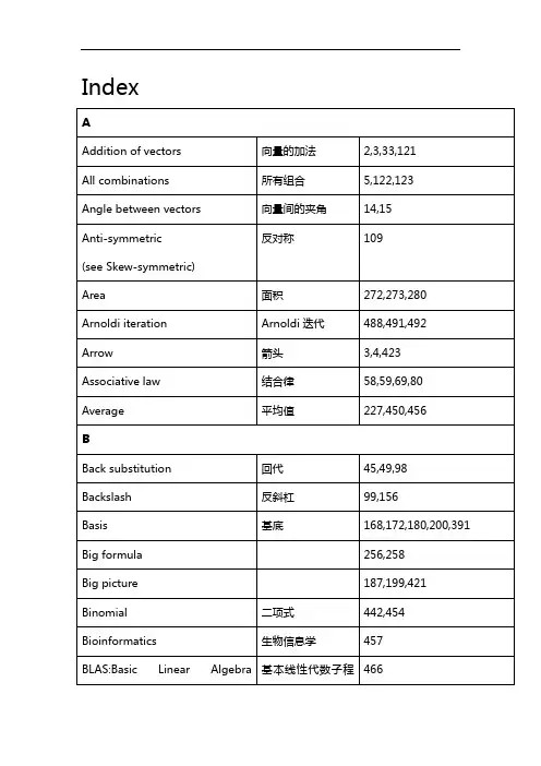
IndexEEconomics 经济学435,439 Eigencourse 457,458Eigenvalue 特征值283,287,374,499 Eigenvalue changes 特征值变换439Eigenvalues of 的特征值284,294,300 Eigenvalues of 的特征值297Eigenvalues of 的特征值362Eigenvector basis 基底的特征向量399Eigenvectors 特征向量283,287,374Eigshow 290,368Elimination 消元法45-66,83,86,135 Ellipse 椭圆290,346,366,382 Energy 能量343,409Engineering 工程409,419Error 误差211,218,219,225,481,483 Error equation 误差方程477Euler angles 欧拉角474Euler’s formula 欧拉公式311,426,430,497Even 偶数113,246,258,452 Exponential 指数的314,319,327FHilbert space 希尔伯特空间447,449Hooke’s Law 虎克定律410,412 Householder reflections 镜像变换237,469,472 Hyperplane 超平面30,42IIll-conditioned matrix 病态矩阵371,473,474 Imaginary 虚数289Independent 独立的26,27,134,168,200,300 Initial value 初值313Inner product 内积11,56,108,448,502,506 Input and output basis 基底输入输出399Integral 积分24,385,386Interior point method 内点法445Intersection of spaces 交空间129,183Inverse matrix 逆矩阵24,81,270Inverse of的逆82Invertible 可逆的86,173,200,248 Iteration 迭代481,482,484,489,492 JJacobi 雅可比481,483,485,489 Jordan form 约当型356,357,358,361,482 JPEG 364,373KKalman filter 卡尔曼滤波器93,214Kernel 核377,380Kirchhoff’s Laws 基尔霍夫定律143,189,420,424-427 Krylov 克雷洛夫491,492Lnorm 和范数225,480Lagrange multiplier 拉格朗日乘子445Lanczos method 兰索斯方法490,492LAPACK 线性代数软件包98,237,486Leapfrog method 跳步法317,329Least squares 最小平方218,219,236,405,408,453 Left nullspace左零空间184,186,192,425Left-inverse 左逆的81,86,154,405Length 长度12,232,447,448,501 Line 线34,40,221,474Line of springs 线弹簧411Linear combination 线性组合1,3Linear equation 线性方程23Linear programming 线性规划440Linear transformation 线性变换44,375-398Linearity 线性关系44,245,246Linearly independent 线性独立26,134,168,169,200 LINPACK 线性系统软件包465Loop 环路307,425,426Lower triangular 下三角9598,100,474Lucas numbers 卢卡斯数306MMaple 38,100Mathematica 38,100MATLAB 17,37,237,243,290,337,513 Matrix(see full page 570) 矩阵22,384,387Matrix exponential 矩阵指数314,319,327Matrix multiplication 矩阵乘法58,59,67,389Matrix notation 矩阵记号37Matrix space 矩阵空间121,122,175,181,311 Matrix 矩阵-1,2,-1 matrix -1,2,-1矩阵106,167,261,265,349,374,410,480Adjacency, 邻接矩阵74,80,311,369All-ones 全1矩阵251,262,307,348 Augmented 增广矩阵60,84,155Band 带状矩阵99,468,469。
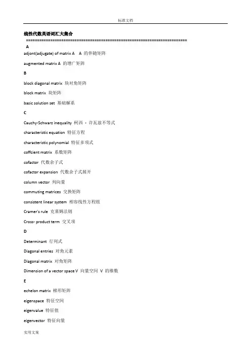
线性代数英语词汇大集合========================================================================= Aadjont(adjugate) of matrix A A 的伴随矩阵augmented matrix A 的增广矩阵Bblock diagonal matrix 块对角矩阵block matrix 块矩阵basic solution set 基础解系CCauchy-Schwarz inequality 柯西- 许瓦兹不等式characteristic equation 特征方程characteristic polynomial 特征多项式coffcient matrix 系数矩阵cofactor 代数余子式cofactor expansion 代数余子式展开column vector 列向量commuting matrices 交换矩阵consistent linear system 相容线性方程组Cramer's rule 克莱姆法则Cross- product term 交叉项DDeterminant 行列式Diagonal entries 对角元素Diagonal matrix 对角矩阵Dimension of a vector space V 向量空间V 的维数Eechelon matrix 梯形矩阵eigenspace 特征空间eigenvalue 特征值eigenvector 特征向量eigenvector basis 特征向量的基elementary matrix 初等矩阵elementary row operations 行初等变换Ffull rank 满秩fundermental set of solution 基础解系Ggrneral solution 通解Gram-Schmidt process 施密特正交化过程Hhomogeneous linear equations 齐次线性方程组Iidentity matrix 单位矩阵inconsistent linear system 不相容线性方程组indefinite matrix 不定矩阵indefinit quatratic form 不定二次型infinite-dimensional space 无限维空间inner product 内积inverse of matrix A 逆矩阵JKLlinear combination 线性组合linearly dependent 线性相关linearly independent 线性无关linear transformation 线性变换lower triangular matrix 下三角形矩阵Mmain diagonal of matrix A 矩阵的主对角matrix 矩阵Nnegative definite quaratic form 负定二次型negative semidefinite quadratic form 半负定二次型nonhomogeneous equations 非齐次线性方程组nonsigular matrix 非奇异矩阵nontrivial solution 非平凡解norm of vector V 向量V 的范数normalizing vector V 规范化向量Oorthogonal basis 正交基orthogonal complemen t 正交补orthogonal decomposition 正交分解orthogonally diagonalizable matrix 矩阵的正交对角化orthogonal matrix 正交矩阵orthogonal set 正交向量组orthonormal basis 规范正交基orthonomal set 规范正交向量组Ppartitioned matrix 分块矩阵positive definite matrix 正定矩阵positive definite quatratic form 正定二次型positive semidefinite matrix 半正定矩阵positive semidefinite quadratic form 半正定二次型Qquatratic form 二次型Rrank of matrix A 矩阵A 的秩r(A )reduced echelon matrix 最简梯形阵row vector 行向量Sset spanned by { } 由向量{ } 所生成similar matrices 相似矩阵similarity transformation 相似变换singular matrix 奇异矩阵solution set 解集合standard basis 标准基standard matrix 标准矩阵Isubmatrix 子矩阵subspace 子空间symmetric matrix 对称矩阵Ttrace of matrix A 矩阵A 的迹tr ( A )transpose of A 矩阵A 的转秩triangle inequlity 三角不等式trivial solution 平凡解Uunit vector 单位向量upper triangular matrix 上三角形矩阵Vvandermonde matrix 范得蒙矩阵vector 向量vector space 向量空间WZzero subspace 零子空间zero vector 零空间==============================================================================向量:vector 向量的长度(模):零向量: zero vector负向量: 向量的加法:addition 三角形法则:平行四边形法则:多边形法则减法向量的标量乘积:scalar multiplication 向量的线性运算线性组合:linear combination 线性表示,线性相关(linearly dependent),线性无关(linearly independent),原点(origin)位置向量(position vector)线性流形(linear manifold)线性子空间(linear subspace)基(basis)仿射坐标(affine coordinates),仿射标架(affine frame),仿射坐标系(affine coordinate system)坐标轴(coordinate axis)坐标平面卦限(octant)右手系左手系定比分点线性方程组(system of linear equations齐次线性方程组(system of homogeneous linear equations)行列式(determinant)维向量向量的分量(component)向量的相等和向量零向量负向量标量乘积维向量空间(vector space)自然基行向量(row vector)列向量(column vector)单位向量(unit vector)直角坐标系(rectangular coordinate system),直角坐标(rectangular coordinates),射影(projection)向量在某方向上的分量,正交分解,向量的夹角,内积(inner product)标量积(scalar product),数量积,方向的方向角,方向的方向余弦;二重外积外积(exterior product),向量积(cross product),混合积(mixed product,scalar triple product)==================================================================================(映射(mapping)),(象(image)),(一个原象(preimage)),(定义域(domain)),(值域(range)),(变换(transformation)),(单射(injection)),(象集),(满射(surjection)),(一一映射,双射(bijection)),(原象),(映射的复合,映射的乘积),(恒同映射,恒同变换(identity mapping)),(逆映射(inverse mapping));(置换(permutation)),(阶对称群(symmetric group)),(对换(transposition)),(逆序对),(逆序数),(置换的符号(sign)),(偶置换(even permutation)),(奇置换(odd permutation));行列式(determinant),矩阵(matrix),矩阵的元(entry),(方阵(square matrix)),(零矩阵(zero matrix)),(对角元),(上三角形矩阵(upper triangular matrix)),(下三角形矩阵(lower triangular matrix)),(对角矩阵(diagonal matrix)),(单位矩阵(identity matrix)),转置矩阵(transpose matrix),初等行变换(elementary row transformation),初等列变换(elementary column transformation);(反称矩阵(skew-symmetric matrix));子矩阵(submatrix),子式(minor),余子式(cofactor),代数余子式(algebraic cofactor),(范德蒙德行列式(Vandermonde determinant));(未知量),(系数矩阵),(方程的系数(coefficient)),(常数项(constant)),(线性方程组的解(solution)),(增广矩阵(augmented matrix)),(零解);子式的余子式,子式的代数余子式===================================================================================线性方程组与线性子空间(阶梯形方程组),(方程组的初等变换),行阶梯矩阵(row echelon matrix),主元,简化行阶梯矩阵(reduced row echelon matrix),(高斯消元法(Gauss elimination)),(解向量),(同解),(自反性(reflexivity)),(对称性(symmetry)),(传递性(transitivity)),(等价关系(equivalence));(齐次线性方程组的秩(rank));(主变量),(自由位置量),(一般解),向量组线性相关,向量组线性无关,线性组合,线性表示,线性组合的系数,(向量组的延伸组);线性子空间,由向量组张成的线性子空间;基,坐标,(自然基),向量组的秩;(解空间),线性子空间的维数(dimension),齐次线性方程组的基础解系(fundamental system of solutions);(平面束(pencil of planes))(导出组),线性流形,(方向子空间),(线性流形的维数),(方程组的特解);(方程组的零点),(方程组的图象),(平面的一般方程),(平面的三点式方程),(平面的截距式方程),(平面的参数方程),(参数),(方向向量);(直线的方向向量),(直线的参数方程),(直线的标准方程),(直线的方向系数),(直线的两点式方程),(直线的一般方程);=====================================================================================矩阵的秩与矩阵的运算线性表示,线性等价,极大线性无关组;(行空间,列空间),行秩(row rank),列秩(column rank),秩,满秩矩阵,行满秩矩阵,列满秩矩阵;线性映射(linear mapping),线性变换(linear transformation),线性函数(linear function);(零映射),(负映射),(矩阵的和),(负矩阵),(线性映射的标量乘积),(矩阵的标量乘积),(矩阵的乘积),(零因子),(标量矩阵(scalar matrix)),(矩阵的多项式);(退化的(degenerate)方阵),(非退化的(non-degenerate)方阵),(退化的线性变换),(非退化的线性变换),(逆矩阵(inverse matrix)),(可逆的(invertible),(伴随矩阵(adjoint matrix));(分块矩阵(block matrix)),(分块对角矩阵(block diagonal matrix));初等矩阵(elementary matrix),等价(equivalent);(象空间),(核空间(kernel)),(线性映射的秩),(零化度(nullity))==================================================================================== transpose of matrix 倒置矩阵; 转置矩阵【数学词汇】transposed matrix 转置矩阵【机械专业词汇】matrix transpose 矩阵转置【主科技词汇】transposed inverse matrix 转置逆矩阵【数学词汇】transpose of a matrix 矩阵的转置【主科技词汇】permutation matrix 置换矩阵; 排列矩阵【主科技词汇】singular matrix 奇异矩阵; 退化矩阵; 降秩矩阵【主科技词汇】unitary matrix 单式矩阵; 酉矩阵; 幺正矩阵【主科技词汇】Hermitian matrix 厄密矩阵; 埃尔米特矩阵; 艾米矩阵【主科技词汇】inverse matrix 逆矩阵; 反矩阵; 反行列式; 矩阵反演; 矩阵求逆【主科技词汇】matrix notation 矩阵符号; 矩阵符号表示; 矩阵记号; 矩阵运算【主科技词汇】state transition matrix 状态转变矩阵; 状态转移矩阵【航海航天词汇】torque master 转矩传感器; 转矩检测装置【主科技词汇】spin matrix 自旋矩阵; 旋转矩阵【主科技词汇】moment matrix 动差矩阵; 矩量矩阵【航海航天词汇】Jacobian matrix 雅可比矩阵; 导数矩阵【主科技词汇】relay matrix 继电器矩阵; 插接矩阵【主科技词汇】matrix notation 矩阵表示法; 矩阵符号【航海航天词汇】permutation matrix 置换矩阵【航海航天词汇】transition matrix 转移矩阵【数学词汇】transition matrix 转移矩阵【机械专业词汇】transitionmatrix 转移矩阵【航海航天词汇】transition matrix 转移矩阵【计算机网络词汇】transfer matrix 转移矩阵【物理词汇】rotation matrix 旋转矩阵【石油词汇】transition matrix 转换矩阵【主科技词汇】circulant matrix 循环矩阵; 轮换矩阵【主科技词汇】payoff matrix 报偿矩阵; 支付矩阵【主科技词汇】switching matrix 开关矩阵; 切换矩阵【主科技词汇】method of transition matrices 转换矩阵法【航海航天词汇】stalling torque 堵转力矩, 颠覆力矩, 停转转矩, 逆转转矩【航海航天词汇】thin-film switching matrix 薄膜转换矩阵【航海航天词汇】rotated factor matrix 旋转因子矩阵【航海航天词汇】transfer function matrix 转移函数矩阵【航海航天词汇】transition probability matrix 转移概率矩阵【主科技词汇】energy transfer matrix 能量转移矩阵【主科技词汇】fuzzy transition matrix 模糊转移矩阵【主科技词汇】canonical transition matrix 规范转移矩阵【主科技词汇】matrix form 矩阵式; 矩阵组织【主科技词汇】stochastic state transition matrix 随机状态转移矩阵【主科技词汇】fuzzy state transition matrix 模糊状态转移矩阵【主科技词汇】matrix compiler 矩阵编码器; 矩阵编译程序【主科技词汇】test matrix 试验矩阵; 测试矩阵; 检验矩阵【主科技词汇】matrix circuit 矩阵变换电路; 矩阵线路【主科技词汇】reducible matrix 可简化的矩阵; 可约矩阵【主科技词汇】matrix norm 矩阵的模; 矩阵模; 矩阵模量【主科技词汇】rectangular matrix 矩形矩阵; 长方形矩阵【主科技词汇】running torque 额定转速时的转矩; 旋转力矩【航海航天词汇】transposed matrix 转置阵【数学词汇】covariance matrix 协变矩阵; 协方差矩阵【主科技词汇】unreduced matrix 未约矩阵; 不可约矩阵【主科技词汇】receiver matrix 接收机矩阵; 接收矩阵变换电路【主科技词汇】torque 传动转矩; 转矩; 阻力矩【航海航天词汇】pull-in torque 启动转矩; 输入转矩, 同步转矩, 整步转矩【航海航天词汇】parity matrix 奇偶校验矩阵; 一致校验矩阵【主科技词汇】bus admittance matrix 母线导纳矩阵; 节点导纳矩阵【主科技词汇】matrix printer 矩阵式打印机; 矩阵形印刷机; 点阵打印机【主科技词汇】dynamic matrix 动力矩阵; 动态矩阵【航海航天词汇】connection matrix 连接矩阵; 连通矩阵【主科技词汇】characteristic matrix 特征矩阵; 本征矩阵【主科技词汇】regular matrix 正则矩阵; 规则矩阵【主科技词汇】flexibility matrix 挠度矩阵; 柔度矩阵【主科技词汇】citation matrix 引文矩阵; 引用矩阵【主科技词汇】relational matrix 关系矩阵; 联系矩阵【主科技词汇】eigenmatrix 本征矩阵; 特征矩阵【主科技词汇】system matrix 系统矩阵; 体系矩阵【主科技词汇】system matrix 系数矩阵; 系统矩阵【航海航天词汇】recovery diode matrix 恢复二极管矩阵; 再生式二极管矩阵【主科技词汇】inverse of a square matrix 方阵的逆矩阵【主科技词汇】torquematic transmission 转矩传动装置【石油词汇】torque balancing device 转矩平衡装置【航海航天词汇】torque measuring device 转矩测量装置【主科技词汇】torque measuring apparatus 转矩测量装置【航海航天词汇】torque-tube type suspension 转矩管式悬置【主科技词汇】steering torque indicator 转向力矩测定仪; 转向转矩指示器【主科技词汇】magnetic dipole moment matrix 磁偶极矩矩阵【主科技词汇】matrix addressing 矩阵寻址; 矩阵寻址时频矩阵编址; 时频矩阵编址【航海航天词汇】stiffness matrix 劲度矩阵; 刚度矩阵; 劲度矩阵【航海航天词汇】first-moment matrix 一阶矩矩阵【主科技词汇】matrix circuit 矩阵变换电路; 矩阵电路【计算机网络词汇】reluctance torque 反应转矩; 磁阻转矩【主科技词汇】pull-in torque 启动转矩; 牵入转矩【主科技词汇】induction torque 感应转矩; 异步转矩【主科技词汇】nominal torque 额定转矩; 公称转矩【航海航天词汇】phototronics 矩阵光电电子学; 矩阵光电管【主科技词汇】column matrix 列矩阵; 直列矩阵【主科技词汇】inverse of a matrix 矩阵的逆; 逆矩阵【主科技词汇】lattice matrix 点阵矩阵【数学词汇】lattice matrix 点阵矩阵【物理词汇】canonical matrix 典型矩阵; 正则矩阵; 典型阵; 正则阵【航海航天词汇】moment matrix 矩量矩阵【主科技词汇】moment matrix 矩量矩阵【数学词汇】dynamic torque 动转矩; 加速转矩【主科技词汇】indecomposable matrix 不可分解矩阵; 不能分解矩阵【主科技词汇】printed matrix wiring 印刷矩阵布线; 印制矩阵布线【主科技词汇】decoder matrix circuit 解码矩阵电路; 译码矩阵电路【航海航天词汇】scalar matrix 标量矩阵; 标量阵; 纯量矩阵【主科技词汇】array 矩阵式组织; 数组; 阵列【计算机网络词汇】commutative matrix 可换矩阵; 可交换矩阵【主科技词汇】标准文档实用文案。
1linear equation [P2] 线性方程coefficient [P2] 系数constant term [讲义‐P1] 常数(项)systems of linear equations (linear system) [P3] 线性方程组solution [P3] 解solution set [P3] 解集tuple [P3] 数组equivalent [P3] 等价equivalent system [P3] 等价系统,等价方程组 consistent [P4] 相容inconsistent [P4] 不相容consistent linear system 相容(有解)的线性方程组inconsistent linear system 不相容(无解)的线性方程组coefficient matrix [P5] 系数矩阵augmented matrix [P5] 增广矩阵elementary operations [P7] 初等变换elementary row operation [P7] 初等行变换row equivalent [P7] 行等价(矩阵) equivalent matrix [讲义‐P3] 等价矩阵Leading entry [P14] 先导元素entry of matrix 矩阵的元素echelon form (row echelon form) [P14] 阶梯形reduced echelon form (reduced row echelon form) [P14] 简化阶梯形Gaussian elimination [P14]脚注 高斯消元法the elimination of variables 消元法row reduced [P15] 行化简pivot position [P16] 主元位置pivot column [P16] 主元列pivot [P17] 主元forward phase [P20] 自上(向下)阶段 backward phase [P20] 自下(向上)阶段basic variable [P20] 基本变元free variable [P20] 自由变元general solution [P21] 一般解,通解back‐substitution [P22] 回代法,侧转代入vector [P28] 向量, 矢量scalar [P28] 数量,纯量, 无向量 parallelogram rule [P30] 平行四边形法则linear combination [P32] 线性组合generated (spanned) [P35] 生成(张成)product [P45] 乘积homogeneous systems [P50] 齐次系统,齐次线性方程组 trivial solution [P50] 平凡解,零解nontrivial solution [P51] 非平凡解, 非零解 parametric vector form [P52] 参数向量形式 nonhomogeneous systems [P50] 非齐次线性方程组linear independent [p65] 线性相关linearly independent [P65] 线性无关linear transformation [P73] 线性变换domain [P73] 值域shear transformation [P76] 剪切变换contraction [P77] 压缩变换dilation [P77] 拉伸变换。
英汉词汇(按英文字母排序)Aadjont(adjugate) of matrix A A 的伴随矩阵augmented matrix A 的增广矩阵Bblock diagonal matrix 块对角矩阵block matrix 块矩阵basic solution set 基础解系CCauchy-Schwarz inequality 柯西 - 许瓦兹不等式characteristic equation 特征方程characteristic polynomial 特征多项式coffcient matrix 系数矩阵cofactor 代数余子式cofactor expansion 代数余子式展开column vector 列向量commuting matrices 交换矩阵consistent linear system 相容线性方程组Cramer's rule 克莱姆法则Cross- product term 交叉项DDeterminant 行列式Diagonal entries 对角元素Diagonal matrix 对角矩阵Dimension of a vector space V 向量空间V 的维数Eechelon matrix 梯形矩阵eigenspace 特征空间eigenvalue 特征值eigenvector 特征向量eigenvector basis 特征向量的基elementary matrix 初等矩阵elementary row operations 行初等变换Ffull rank 满秩fundermental set of solution 基础解系Ggrneral solution 通解Gram-Schmidt process 施密特正交化过程Hhomogeneous linear equations 齐次线性方程组Iidentity matrix 单位矩阵inconsistent linear system 不相容线性方程组indefinite matrix 不定矩阵indefinit quatratic form 不定二次型infinite-dimensional space 无限维空间inner product 内积inverse of matrix A 逆矩阵JKLlinear combination 线性组合linearly dependent 线性相关linearly independent 线性无关linear transformation 线性变换lower triangular matrix 下三角形矩阵Mmain diagonal of matrix A 矩阵的主对角matrix 矩阵Nnegative definite quaratic form 负定二次型negative semidefinite quadratic form 半负定二次型nonhomogeneous equations 非齐次线性方程组nonsigular matrix 非奇异矩阵nontrivial solution 非平凡解norm of vector V 向量 V 的范数normalizing vector V 规范化向量Oorthogonal basis 正交基orthogonal complemen t 正交补orthogonal decomposition 正交分解orthogonally diagonalizable matrix 矩阵的正交对角化orthogonal matrix 正交矩阵orthogonal set 正交向量组orthonormal basis 规范正交基orthonomal set 规范正交向量组Ppartitioned matrix 分块矩阵positive definite matrix 正定矩阵positive definite quatratic form 正定二次型positive semidefinite matrix 半正定矩阵positive semidefinite quadratic form 半正定二次型Qquatratic form 二次型Rrank of matrix A 矩阵A 的秩r(A )reduced echelon matrix 最简梯形阵row vector 行向量Sset spanned by { } 由向量 { } 所生成similar matrices 相似矩阵similarity transformation 相似变换singular matrix 奇异矩阵solution set 解集合standard basis 标准基standard matrix 标准矩阵Isubmatrix 子矩阵subspace 子空间symmetric matrix 对称矩阵Ttrace of matrix A 矩阵A 的迹tr ( A ) transpose of A 矩阵A 的转秩triangle inequlity 三角不等式trivial solution 平凡解Uunit vector 单位向量upper triangular matrix 上三角形矩阵Vvandermonde matrix 范得蒙矩阵vector 向量vector space 向量空间WZzero subspace 零子空间zero vector 零空间。