Numbers of edges in supermagic graphs

18.06 Linear Algebra, Spring 2005Please use the following citation format:Gilbert Strang, 18.06 Linear Algebra, Spring 2005. (MassachusettsInstitute of Technology: MIT OpenCourseWare). (accessed MM DD, YYYY). License: Creative Commons Attribution-Noncommercial-Share Alike.Note: Please use the actual date you accessed this material in your citation. For more information about citing these materials or our Terms of Use, visit: /terms18.06 Linear Algebra, Spring 2005Transcript – Lecture 12OK. This is lecture twelve.We've reached twelve lectures. And this one is more than the others about applications of linear algebra.And I'll confess. When I'm giving you examples of the null space and the row space, I create a little matrix. You probably see that I just invent that matrix as I'm going.And I feel a little guilty about it, because the truth is that real linear algebra uses matrices that come from somewhere. They're not just, like, randomly invented by the instructor.They come from applications. They have a definite structure.And anybody who works with them gets, uses that structure.I'll just report, like, this weekend I was at an event with chemistry professors. OK, those guys are row reducing matrices, and what matrices are they working with? Well, their little matrices tell them how much of each element goes into the --or each molecule, how many molecules of each go into a reaction and what comes out. And by row reduction they get a clearer picture of a complicated reaction. And this weekend I'm going to --to a sort of birthday party at Mathworks. So Mathworks is out Route 9 in Natick.That's where Matlab is created. It's a very, very successful, software, tremendously successful. And the conference will be about how linear algebra is used. And so I feel better today to talk about what I think is the most important model in applied math. And the discrete version is a graph. So can I draw a graph? Write down the matrix that's associated with it, and that's a great source of matrices. You'll see. So a graph is just, so a graph --to repeat --has nodes and edges. OK.And I'm going to write down the graph, a graph, so I'm just creating a small graph here.As I mentioned last time, we would be very interested in the graph of all, websites.Or the graph of all telephones. I mean --or the graph of all people in the world. Here let me take just, maybe nodes one two three --well, I better put in an --I'll put in that edge and maybe an edge to, to a node four, and another edge to node four. How's that? So there's a graph with four nodes.So n will be four in my --n equal four nodes.And the matrix will have m equal the number --there'll be a row for every edge, so I've got one two three four five edges. So that will be the number of rows. And I have to to write down the matrix that I want to, I want to study, I need to give a direction to every edge, so I know a plus and a minus direction. So I'll just do that with an arrow. Say from one to two, one to three, two to three, one to four, three to four.That just tells me, if I have current flowing on these edges then I know whether it's --to count it as positive or negative according as whether it's with the arrow or against the arrow. But I just drew those arrows arbitrarily. OK.Because I --my example is going to come --the example I'll --the words that I will use will be words like potential, potential difference, currents. In other words, I'm thinking of an electrical network.But that's just one possibility.My applied math class builds on this example.It could be a hydraulic network, so we could be doing, flow of water, flow of oil. Other examples, this could be a structure.Like the --a design for a bridge or a design for a Buckminster Fuller dome. Or many other possibilities, so many. So l-but let's take potentials and currents as, as a basic example, and let me create the matrix that tells you exactly what the graph tells you. So now I'll call it the incidence matrix, incidence matrix. OK. So let me write it down, and you'll see, what its properties are.So every row corresponds to an edge.I have five rows from five edges, and let me write down again what this graph looks like.OK, the first edge, edge one, goes from node one to two. So I'm going to put in a minus one and a plus one in th-this corresponds to node one two three and four, the four columns. The five rows correspond --the first row corresponds to edge one. Edge one leaves node one and goes into node two, and that --and it doesn't touch three and four.Edge two, edge two goes --oh, I haven't numbered these edges.I just figured that was probably edge one, but I didn't say so. Let me take that to be edge one. Let me take this to be edge two. Let me take this to be edge three. This is edge four. Ho, I'm discovering --no, wait a minute.Did I number that twice? Here's edge four. And here's edge five. OK? All right. So, so edge one, as I said, goes from node one to two.Edge two goes from two to three, node two to three, so minus one and one in the second and third columns.Edge three goes from one to three.I'm, I'm tempted to stop for a moment with those three edges.Edges one two three, those form what would we, what do you call the, the little, the little, the subgraph formed by edges one, two, and three? That's a loop. And the number of loops and the position of the loops will be crucial.OK. Actually, here's a interesting point about loops. If I look at those rows, corresponding to edges one two three, and these guys made a loop. You want to tell me --if I just looked at that much of the matrix it would be natural for me to ask, are those rows independent? Are the rows independent? And can you tell from looking at that if they are or are not independent? Do you see a, a relation between those three rows? Yes.If I add that row to that row, I get this row.So, so that's like a hint here that loops correspond to dependent, linearly dependent column --linearly dependent rows. OK, let me complete the incidence matrix. Number four, edge four is going from node one to node four.And the fifth edge is going from node three to node four.OK. There's my matrix.It came from the five edges and the four nodes.And if I had a big graph, I'd have a big matrix.And what questions do I ask about matrices? Can I ask --here's the review now. There's a matrix that comes from somewhere.If, if it was a big graph, it would be a large matrix, but a lot of zeros, right? Because every row only has two non-zeros.So the number of --it's a very sparse matrix.The number of non-zeros is exactly two times five, it's two m. Every row only has two non-zeros. And that's with a lot of structure. And --that was the point I wanted to begin with, that graphs, that real graphs from real --real matrices from genuine problems have structure. OK.We can ask, and because of the structure, we can answer, the, the main questions about matrices.So first question, what about the null space? So what I asking if I ask you for the null space of that matrix? I'm asking you if I'm looking at the columns of the matrix, four columns, and I'm asking you, are those columns independent? If the columns are independent, then what's in the null space? Only the zero vector, right? The null space contains --tells us what combinations of the columns --it tells us how to combine columns to get zero.Can --and is there anything in the null space of this matrix other than just the zero vector? In other words, are those four columns independent or dependent? OK.That's our question.Let me, I don't know if you see the answer.Whether there's --so let's see.I guess we could do it properly. We could solve Ax=0. So let me solve Ax=0 to find the null space. OK.What's Ax? Can I put x in here in, in little letters? x1, x2, x3, x4, that's --it's got four columns.Ax now is that matrix times x. And what do I get for Ax? If the camera can keep that matrix multiplication there, I'll put the answer here. Ax equal --what's the first component of Ax? Can you take that first row, minus one one zero zero, and multiply by the x, and of course you get x2-x1. The second row, I get x3-x2. From the third row, I get x3-x1. From the fourth row, I get x4-x1. And from the fifth row, I get x4-x3. And I want to know when is the thing zero. This is my equation, Ax=0. Notice what that matrix A is doing, what we've created a matrix that computes the differences across every edge, the differences in potential.Let me even begin to give this interpretation.I'm going to think of this vector x, which is x1 x2 x3 x4, as the potentials at the nodes. So I'm introducing a word, potentials at the nodes. And now if I multiply by A, I get these --I get these five components, x2-x1, et cetera. And what are they? They're potential differences. That's what A computes.If I have potentials at the nodes and I multiply by A, it gives me the potential differences, the differences in potential, across the edges. OK.When are those differences all zero? So I'm looking for the null space.Of course, if all the (x)s are zero then I get zero.That, that just tells me, of course, the zero vector is in the null space. But w-there's more in the null space. Those columns are --of A are dependent, right --because I can find solutions to that equation. Tell me --the null space.Tell me one vector in the null space, so tell me an x, it's got four components, and it makes that thing zero.So what's a good x to do that? One one one one, constant potential. If the potentials are constant, then all the potential differences are zero, and that x is in the null space.What else is in the null space? If it --yeah, let me ask you just always, give me a basis for the null space. A basis for the null space will be just that.1 That's --, that's it.That's a basis for the null space.The null space is actually one dimensional, and it's the line of all vectors through that one. So there's a basis for it, and here is the whole null space.Any multiple of one one one one, it's the whole line in four dimensional space. Do you see that that's the null space? So the, so the dimension of the null space of A is one. And there's a basis for it, and there's everything that's in it.Good. And what does that mean physically? I mean, what does that mean in the application? That guy in the null space.It means that the potentials can only be determined up to a constant. Potential differences are what make current flow. That's what makes things happen. It's these potential differences that will make something move in the, in our network, between x2-between node two and node one. Nothing will move if all potentials are the same. If all potentials are c, c, c, and c, then nothing will move. So we're, we have this one parameter, this arbitrary constant that raises or drops all the potentials.It's like ranking football teams, whatever.We have a, there's a, there's a constant --or looking at temperatures, you know, there's a flow of heat from higher temperature to lower temperature. If temperatures are equal there's no flow, and therefore we can measure --we can measure temperatures by, Celsius or we can start at absolute zero.And that arbitrary --it's the same arbitrary constant that, that was there in calculus. In calculus, right, when you took the integral, the indefinite integral, there was a plus c, and you had to set a starting point to know what that c was. So here what often happens is we fix one of the potentials, like the last one.So a typical thing would be to ground that node.To set its potential at zero. And if we do that, if we fix that potential so it's not unknown anymore, then that column disappears and we have three columns, and those three columns are independent.So I'll leave the column in there, but we'll remember that grounding a node is the way to get it out.And grounding a node is the way to --setting a node --setting a potential to zero tells us the, the base for all potentials. Then we can compute the others. OK. But what's the --now I've talked enough to ask what the rank of the matrix is? What's the rank then? The rank of the matrix.So we have a five by four matrix.We've located its null space, one dimensional.How many independent columns do we have? What's the rank? It's three.And the first three columns, or actually any three columns, will be independent. Any three potentials are independent, good variables. The fourth potential is not, we need to set, and typically we ground that node. OK.Rank is three. Rank equals three.OK. Let's see, do I want to ask you about the column space? The column space is all combinations of those columns. I could say more about it and I will. Let me go to the null space of A transpose, because the equation A transpose y equals zero is probably the most fundamental equation of applied mathematics. All right, let's talk about that. That deserves our attention. A transpose y equals zero. Let's --let me put it on here. OK. So A transpose y equals zero.So now I'm finding the null space of A transpose.Oh, and if I ask you its dimension, you could tell me what it is. What's the dimension of the null space of A transpose? We now know enough to answer that question. What's the general formula for the dimension of the null space of A transpose? A transpose, let me even write out A transpose. This A transpose will be n by m, right? n by m.In this case, it'll be four by five.Those columns will become rows. Minus one zero minus one minus one zero is now the first row. The second row of the matrix, one minus one and three zeros. The third column now becomes the third row, zero one one zero minus one. And the fourth column becomes the fourth row.OK, good. There's A transpose.That multiplies y, y1 y2 y3 y4 and y5.OK. Now you've had time to think about this question. What's the dimension of the null space, if I set all those --wow.Usually --sometime during this semester, I'll drop one of these erasers behind there. That's a great moment.There's no recovery. There's --centuries of erasers are back there. OK. OK, what's the dimension of the null space? Give me the general formula first in terms of r and m and n.This is like crucial, you --we struggled to, to decide what dimension meant, and then we figured out what it equaled for an m by n matrix of rank r, and the answer wasm-r, right? There are m=5 components, m=5 columns of A transpose. And r of those columns are pivot columns, because it'll have r pivots.It has rank r. And m-r are the free ones now for A transpose, so that's five minus three, so that's two. And I would like to find this null space. I know its dimension. Now I want to find out a basis for it.And I want to understand what this equation is.So let me say what A transpose y actually represents, why I'm interested in that equation.I'll put it down with those old erasers and continue this.Here's the great picture of applied mathematics.So let me complete that. There's a matrix that I'll call C that connects potential differences to currents.So I'll call these --these are currents on the edges, y1 y2 y3 y4 and y5. Those are currents on the edges. And this relation between current and potential difference is Ohm's Law.This here is Ohm's Law. Ohm's Law says that the current on an edge is some number times the potential drop. That's --and that number is the conductance of the edge, one over the resistance. This is the old current is, is, the relation of current, resistance, and change in potential. So it's a change in potential that makes some current happen, and it's Ohm's Law that says how much current happens. OK.And then the final step of this framework is the equation A transpose y equals zero. And that's --what is that saying? It has a famous name.It's Kirchoff's Current Law, KCL, Kirchoff's Current Law, A transpose y equals zero. So that when I'm solving, and when I go back up with this blackboard and solve A transpose y equals zero, it's this pattern of --that I want you to see. That we had rectangular matrices, but --and real applications, but in those real applications comes A and A transpose.So our four subspaces are exactly the right things to know about. All right.Let's know about that null space of A transpose.Wait a minute, where'd it go? There it is. OK.OK. Null space of A transpose.We know what its dimension should be.Let's find out --tell me a vector in it.Tell me --now, so what I asking you? I'm asking you for five currents that satisfy Kirchoff's Current Law. So we better understand what that law says. That, that law, A transpose y equals zero, what does that say, say in the first row of A transpose? That says --the so the first row of A transpose says minus y1 minus y3 minus y4 is zero. Where did that equation come from? Let me --I'll redraw the graph. Can I redraw the graph here, so that we --maybe here, so that we see again --there was node one, node two, node three, node four was off here. That was, that was our graph.We had currents on those. We had a current y1 going there. We had a current y --what were the other, what are those edge numbers? y4 here and y3 here. And then a y2 and a y5.I'm, I'm just copying what was on the other board so it's ea-convenient to see it. What is this equation telling me, this first equation of Kirchoff's Current Law? What does that mean for that graph? Well, I see y1, y3, and y4 as the currents leaving node one. So sure enough, the first equation refers to node one, and what does it say? It says that the net flow is zero.That, that equation A transpose y, Kirchoff's Current Law, is a balance equation, a conservation law.Physicists, be overjoyed, right, by this stuff.It, it says that in equals out. And in this case, the three arrows are all going out, so it says y1, y3, and y4 add to zero. Let's take the next one.The second row is y1-y2, and that's all that's in that row. And that must have something to do with node two. And sure enough, it says y1=y2, current in equals current out. The third one, y2 plus y3 minus y5 equals zero. That certainly will be what's up at the third node. y2 coming in, y3 coming in, y5 going out has to balance. And finally, y4 plus y5 equals zero says that at this node, y4 plus y5, the total flow, is zero. We don't --you know, charge doesn't accumulate at the nodes.It travels around. OK.Now give me --I come back now to the linear algebra question.What's a vector y that solves these equations? Can I figure out what the null space is for this matrix, A transpose, by looking at the graph? I'm happy if I don't have to do elimination. I can do elimination, we know how to do, we know how to find the null space basis.We can do elimination on this matrix, and we'll get it into a good reduced row echelon form, and the special solutions will pop right out. But I would like to --even to do it without that. Let me just ask you first, if I did elimination on that, on that, matrix, what would the last row become? What would the last row --if I do elimination on that matrix, the last row of R will be all zeros, right? Why? Because the rank is three. We only going to have three pivots. And the fourth row will be all zeros when we eliminate. So elimination will tell us what, what we spotted earlier, what's the null space --all the, all the information, what are the dependencies. We'll find those by elimination, but here in a real example, we can find them by thinking. OK. Again, my question is, what is a solution y? How could current travel around this network without collecting any charge at the nodes? Tell me a y. OK.So a basis for the null space of A transpose.How many vectors I looking for? Two.It's a two dimensional space. My basis should have two vectors in it. Give me one. One set of currents. Suppose, let me start it.Let me start with y1 as one. OK.So one unit of --one amp travels on edge one with the arrow. OK, then what? What is y2? It's one also, right? And of course what you did was solve Kirchoff's Current Law quickly in the second equation.OK. Now we've got one amp leaving node one, coming around to node three.What shall we do now? Well, what shall I take for y3 in other words? Oh, I've got a choice, but why not make it what you said, negative one.So I have just sent current, one amp, around that loop.What shall y4 and y5 be in this case? We could take them to be zero. This satisfies Kirchoff's Current Law. We could check it patiently, that minus y1 minus y3 gives zero.We know y1 is y2. The others, y4 plus y5 is certainly zero. Any current around a loop satisfies --satisfies the Current Law. OK. Now you know how to get another one. Take current around this loop. So now let y3 be one, y5 be one, and y4 be minus one.And so, so we have the first basis vector sent current around that loop, the second basis vector sends current around that loop. And I've --and those are independent, and I've got two solutions --two vectors in the null space of A transpose, two solutions to Kirchoff's Current Law.Of course you would say what about sending current around the big loop. What about that vector? One for y1, one for y2, nothing f-on y3, one for y5, and minus one for y4. What about that? Is that, is that in the null space of A transpose? Sure. So why don't we now have a third vector in the basis? Because it's not independent, right? It's not independent. This vector is the sum of those two. If I send current around that and around that --then on this edge y3 it's going to cancel out and I'll have altogether current around the whole, the outside loop. That's what this one is, but it's a combination of those two.Do you see that I've now, I've identified the null space of A transpose --but more than that, we've solved Kirchoff's Current Law.And understood it in terms of the network.OK. So that's the null space of A transpose. I guess I --there's always one more space to ask you about. Let's see, I guess I need the row space of A, the column space of A transpose. So what's N, what's its dimension? Yup? What's the dimension of the row space of A? If I look at the original A, it had five rows.How many were independent? Oh, I guess I'm asking you the rank again, right? And the answer is three, right? Three independent rows. When I transpose it, there's three independent columns. Are those columns independent, those three? The first three columns, are they the pivot columns of the matrix? No. Those three columns are not independent. There's a in fact, this tells me a relation between them. There's a vector in the null space that says the first column plus the second column equals the third column.They're not independent because they come from a loop. So the pivot columns, the pivot columns of this matrix will be the first, the second, not the third, but the fourth. One, columns one, two, and four are OK. Where are they --those are the columns of A transpose, those correspond to edges.So there's edge one, there's edge two, and there's edge four. So there's a --that's like --is a, smaller graph.If I just look at the part of the graph that I've, that I've, thick --used with thick edges, it has the same four nodes. It only has three edges.And the, those edges correspond to the independent guys. And in the graph there --those three edges have no loop, right? The independent ones are the ones that don't have a loop. All the --dependencies came from loops. They were the things in the null space of A transpose. If I take three pivot columns, there are no dependencies among them, and they form a graph without a loop, and I just want to ask youwhat's the name for a graph without a loop? So a graph without a loop is --has got not very many edges, right? I've got four nodes and it only has three edges, and if I put another edge in, I would have a loop. So it's this graph with no loops, and it's the one where the rows of A are independent.And what's a graph called that has no loops? It's called a tree. So a tree is the name for a graph with no loops. And just to take one last step here. Using our formula for dimension. Using our formula for dimension, let's look --once at this formula.The dimension of the null space of A transpose is m-r.OK. This is the number of loops, number of independent loops. m is the number of edges.And what is r? What is r for our --we'll have to remember way back. The rank came --from looking at the columns of our matrix. So what's the rank? Let's just remember. Rank was --you remember there was one --we had a one dimensional --rank was n minus one, that's what I'm struggling to say. Because there were n columns coming from the n nodes, so it's minus, the number of nodes minus one, because of that C, that one one one one vector in the null space.The columns were not independent.There was one dependency, so we needed n minus one.This is a great formula. This is like the first shall I, --write it slightly differently? The number of edges --let me put things --have I got it right? Number of edges is m, the number --r-is m-r, OK. So, so I'm getting --let me put the number of nodes on the other side. So I --the number of nodes --I'll move that to the other side --minus the number of edges plus the number of loops is --I have minus, minus one is one.The number of nodes minus the number of edges plus the number of loops is one. These are like zero dimensional guys. They're the points on the graph. The edges are like one dimensional things, they're, they connect nodes. The loops are like two dimensional things. They have, like, an area. And this count works for every graph.And it's known as Euler's Formula.We see Euler again, that guy never stopped.OK. And can we just check --so what I saying? I'm saying that linear algebra proves Euler's Formula. Euler's Formula is this great topology fact about any graph. I'll draw, let me draw another graph, let me draw a graph with more edges and loops. Let me put in lots of --OK. I just drew a graph there.So what are the, what are the quantities in that formula? How many nodes have I got? Looks like five. How many edges have I got? One two three four five six seven. How many loops have I got? One two three.And Euler's right, I always get one.That, this formula, is extremely useful in understanding the relation of these quantities --the number of nodes, the number of edges, and the number of loops. OK.Just complete this lecture by completing this picture, this cycle. So let me come to the --so this expresses the equations of applied math. This, let me call these potential differences, say, E. So E is A x.That's the equation for this step.The currents come from the potential differences. y is C E. The potential --the currents satisfy Kirchoff's Current Law. Those are the equations of --with no source terms. Those are the equations of electrical circuits of many --those are like the, the most basic three equations. Applied math comes in this structure. The only thing I haven't got yet in the picture is an outside source to make something happen.I could add a current source here, I could, I could add external currents going in and out of nodes.I could add batteries in the edges.Those are two ways. If I add batteries in the edges, they, they come into here.Let me add current sources. If I add current sources, those come in here. So there's a, there's where current sources go, because the F is a like a current coming from outside. So we have our edges, we have our graph, and then I send one amp into this node and out of this node --and that gives me, a right-hand side in Kirchoff's Current Law. And can I --to complete the lecture, I'm just going to put these three equations together.So I start with x, my unknown.I multiply by A. That gives me the potential differences. That was our matrix A that the whole thing started with. I multiply by C.Those are the physical constants in Ohm's Law.。

负权边的单源最短路问题解决方法Dealing with the negative weight edge single-source shortest path problem can be challenging, but there are several effective methods to tackle this issue. One of the most commonly used algorithms for this problem is the Bellman-Ford algorithm, which can handle graphs with negative weight edges by detecting and updating the shortest paths iteratively. The algorithm is designed to accommodate negative weight edges by allowing for relaxation of edges multiple times until the shortest paths are determined. However, it is important to note that the Bellman-Ford algorithm has a time complexity of O(VE), where V is the number of vertices and E is the number of edges, which can make it less efficient for large graphs.解决负权边的单源最短路径问题可能是具有挑战性的，但有几种有效的方法可以应对这个问题。

其中最常用的算法之一是贝尔曼-福特算法，该算法可以通过迭代地检测和更新最短路径来处理带有负权边的图。

五、树上删边游戏1．游戏规则从某一棵树上删除一条边，同时删去所有在删除边后不再与根相连的部分。

双方轮流进行，无法再进行删除者判定为失败，也就是比你拿掉最后一部分你就赢了。

一个游戏中有多棵树，我们把它们的根都挂在天花板上…或者说，放在地板上也行..这么做是为了方便后面的一些解释和处理。

在这篇文章中，我们讨论的将是公平游戏，也就是双方可以删除任意的边，我们称这个游戏为：Green Hackenbush，暂且称之为树上公平删边游戏。

这个命名是因为还有另外一种删边游戏，为不公平的，参与者双方一方只能删除蓝色边，一方只能删除红色边，而绿色边是两边都可以删除的。

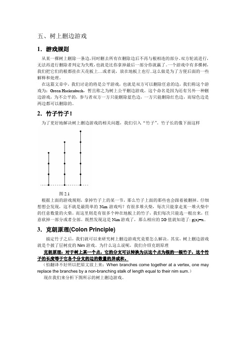
2．竹子竹子！为了更好地解决树上删边游戏的相关问题，我们引入“竹子”。

竹子长的像下面这样图2.1根据上面的游戏规则，拿掉竹子上的某一节，那么竹子上面的那些也会跟着被删掉。

仔细想想会发现，这不就是最简单的Nim游戏吗？有很多堆火柴，每次只能拿走某一堆火柴中的任意数量的火柴。

而这里则是有很多个种在地板上的竹子，我们每次只能选一根出来，任意砍掉一部分或者全部。

既然发现这是Nim游戏了，那么相应的SG值就知道了: g(x)=x..3．克朗原理(Colon Principle)搞定竹子之后，我们就可以来研究树上删边游戏究竟要怎么解决。

其实，树上删边游戏就是个披了层树皮的Nim游戏。

为什么这么说呢，我们介绍克朗原理克朗原理：对于树上某一个点，它的分支可以转换为以这个点为根的一根竹子，这个竹子的长度等于它各个分支的边的数量的异或和。

（怕翻译不好所以把原文放上来：When branches come together at a vertex, one may replace the branches by a non-branching stalk of length equal to their nim sum.）现在我们来分析下图所示的树上删边游戏。

图3.1对于第一个图，1号点有2个分支，分支上的边树分别为1、1，异或和为0，所以1号点的分支被替换为长度为0的竹子，也就是说上面两个分支被删掉了。

edge flages 数学公式
在几何学和计算机图形学中，边缘刻度是一种重要的概念，它被广泛应用于各种图形处理和图像识别任务中。

而Edge Flages数学公式则是一种计算边缘刻度的方法，它可以轻松帮助我们求解各种图形的边缘刻度值。

Edge Flages数学公式的具体计算方法如下：
1. 首先，我们需要计算出每个顶点的度数，即与该顶点相邻的边的数量。

2. 然后，我们根据欧拉公式 V - E + F = 2，其中V表示顶点数，E表示边数，F表示面数，来计算出图形的面数。

3. 接下来，我们根据以下公式计算出每个顶点的边缘刻度值： edge flages value = (2 - degree of the vertex + adjacent edge flages values) / number of adjacent edges
其中，degree of the vertex表示该顶点的度数，adjacent edge flages values表示与该顶点相邻的顶点的边缘刻度值之和，number of adjacent edges表示与该顶点相邻的边的数量。

4. 最后，我们可以根据每个顶点的边缘刻度值来进行各种图形处理和图像识别任务。

掌握Edge Flages数学公式不仅可以帮助我们更好地理解图形的结构和特性，还可以在各种实际应用中发挥重要作用。

- 1 -。

强连通分量的英文Strongly Connected ComponentsIn the realm of graph theory, the concept of strongly connected components (SCCs) plays a pivotal role in understanding the intricate relationships and structures within a directed graph. A strongly connected component is a subgraph of a directed graph in which every pair of vertices is reachable from one another, meaning that there exists a directed path between any two vertices in the component.The identification and analysis of strongly connected components have numerous applications in various fields, including computer science, social network analysis, and transportation networks. By understanding the SCCs within a directed graph, we can gain valuable insights into the connectivity and flow of information, resources, or influence within the system.One of the fundamental algorithms used to identify strongly connected components is Kosaraju's algorithm, named after its inventor, Sargent Shunting. This algorithm is a two-pass algorithm that leverages the properties of directed graphs and the concept oftopological sorting to efficiently determine the strongly connected components.The first step of Kosaraju's algorithm involves performing a depth-first search (DFS) on the graph, starting from an arbitrary vertex. During this DFS, the algorithm keeps track of the finishing times of each vertex, meaning the order in which vertices are finished (or fully explored) during the search. This step is crucial, as the finishing times will be used to guide the second pass of the algorithm.In the second step, the algorithm performs another DFS, but this time, it starts from the vertices in the reverse order of their finishing times (i.e., the vertex with the highest finishing time is explored first). This reversed DFS effectively follows the paths in the reverse direction, allowing the algorithm to identify the strongly connected components.The time complexity of Kosaraju's algorithm is O(V+E), where V is the number of vertices and E is the number of edges in the directed graph. This makes it an efficient algorithm for identifying strongly connected components, even in large-scale graphs.Another important algorithm for finding strongly connected components is Tarjan's algorithm, which uses a single depth-first search to identify the SCCs. Tarjan's algorithm is also known for itsefficient use of a stack data structure and the concept of low-link values to determine the strongly connected components.The applications of strongly connected components are vast and diverse. In computer science, SCCs are used in the analysis of control flow in programs, the identification of deadlocks in concurrent systems, and the optimization of database queries. In social network analysis, SCCs can reveal the structure of influential groups and the flow of information within a network. In transportation networks, SCCs can help identify critical junctions or bottlenecks that affect the overall connectivity and efficiency of the system.Furthermore, the study of strongly connected components has led to the development of various graph-related concepts, such as the strongly connected component decomposition, which partitions a directed graph into its strongly connected components and the connections between them. This decomposition can be used to simplify the analysis and visualization of complex directed graphs, making it easier to understand the underlying structures and relationships.In conclusion, strongly connected components are a fundamental concept in graph theory with a wide range of applications. The efficient algorithms, such as Kosaraju's and Tarjan's, for identifying SCCs have contributed significantly to the understanding andanalysis of directed graphs in various domains. As technology and data-driven applications continue to evolve, the importance of strongly connected components in understanding and optimizing complex systems is likely to grow even further.。

Themaximumnumber...The Maximum Number of Edges in aThree-Dimensional Grid-Drawing Prosenjit Bose Jurek Czyzowicz Pat Morin David R.WoodOctober2,2002AbstractAn exact formula is given for the maximum number of edges in a graph that admits a three-dimensional grid-drawing contained in a given bounding box.A three-dimensional(straight-line)grid-drawing of a graph represents the vertices by dis-tinct points in,and represents each edge by a line-segment between its endpoints that does not intersect any other vertex,and does not intersect any other edge except at the endpoints.A folklore result states that every(simple)graph has a three-dimensional grid-drawing(see[2]).We therefore are interested in grid-drawings with small‘volume’.The bounding box of a three-dimensional grid-drawing is the axis-aligned box of min-imum size that contains the drawing.By an grid-drawing we mean a three-dimensional grid-drawing,such that the edges of the bounding box contain,,and grid-points,respectively.The volume of a three-dimensional grid-drawing is the number of grid-points in the bounding box;that is,the volume of an grid-drawing is. (This de?nition is formulated to ensure that a two-dimensional grid-drawing has positive volume.)Our main contribution is the following extremal result.Theorem1.The maximum number of edges in an grid-drawing is exactlyProof.Consider an grid-drawing of a graph with vertices and edges.Let be the set of points contained in the bounding box such that,,and are all integers.Observe that.The midpoint of every edge of is in,and no two edges share a common midpoint.Hence.In addition,the midpoint of an edge does not intersect a vertex.Thus(1)A drawing with the maximum number of edges has no edge that passes through a grid-point.Otherwise,sub-divide the edge,and place the new vertex at that grid-point.Thus ,and,as claimed.This bound is attained by the following construction.Associate a vertex with each grid-point in an grid-box.As illustrated in Figure1,every vertex is adjacent to each of,,,,,, and,unless such a grid-point is not in.It is easily seen that no two edges intersect,except at a common endpoint.Furthermore,every point in is either a vertex or the midpoint of an edge.Thus the number of edges is.Figure1:The neighbourhood of a vertex.Theorem1can be interpreted as a lower bound on the volume of a three-dimensional grid-drawing of a given graph.Many upper bounds on the volume of three-dimensional grid-drawings are known[1–9].There are two known non-trivial lower bounds for speci?c2families of graphs.Cohen,Eades,Lin,and Ruskey[2]proved that the minimum volume of a three-dimensional grid-drawing of the complete graph is.The lower bound follows from the fact that is not planar,and hence at most four vertices can lie in a single grid-plane.The second lower bound is due to Pach,Thiele,and T′o th[7],who proved that the minimum volume of a three-dimensional grid-drawing of the complete bipartite graph is.The proof of the lower bound is based on the observation that no two edges are parallel.The result follows since the number of distinct vectors between adjacent vertices is at most a constant times the volume.The following corollary of Theorem1 generalises this lower bound for to all graphs.Corollary1.A three-dimensional grid-drawing of a graph with vertices and edges has volume greater than.Obviously the bound in Corollary1can be slightly improved by considering the exact dimensions of the boundingbox.Theorem1generalises to multi-dimensional polyline grid-drawings(where edges may bend at grid-points)as follows. Theorem2.Let be a convex set.Let be the set of grid-points in. The maximum number of edges in a polyline grid-drawing with bounding box is at most .If is an grid-box,then the maximum number of edges is exactlyProof.Let.Consider a polyline grid-drawing with bounding box .The midpoint of every edge is in,and no two edges share a common midpoint.A drawing with the maximum number of edges has no edge that passes through a grid-point. Otherwise,sub-divide the edge,and place the new vertex at that grid-point.Thus the number of edges is at most.If is an grid-box,then.To con-struct a grid-drawing with this many edges,associate one vertex with each grid-point in. Observe that every point is in the interior of exactly one unit-sized-dimensional hypercube with corners in,where.For every point,add an edge passing through between opposite vertices of the unit-sized hypercube corresponding to. Edges only intersect at common endpoints,since these unit-sized hypercubes only intersect along their boundaries.Every point in contains a vertex or a midpoint of an edge.Thus the number of edges is precisely.3References[1]T.C ALAMONERI AND A.S TERBINI,3D straight-line grid drawing of4-colorable graphs.Inform.Process.Lett.,63(2):97–102,1997.[2]R.F.C OHEN,P.E ADES,T.L IN,AND F.R USKEY,Three-dimensional graph drawing.Al-gorithmica,17(2):199–208,1996.[3]E.DI G IACOMO,G.L IOTTA,AND S.W ISMATH,Drawing series-parallel graphs on a box.In S.W ISMATH,ed.,Proc.14th Canadian Conf.on Computational Geometry(CCCG’02), The University ofLethbridge,Canada,2002.[4]V.D UJMOVI′C,P.M ORIN,AND D.R.W OOD,Path-width and three-dimensional straight-line grid drawings of graphs.In M.G OODRICH,ed.,Proc.10th International Symp.on Graph Drawing(GD’02),Lecture Notes in Comput.Sci.,Springer,to appear.[5]V.D UJMOVI′C AND D.R.W OOD,Tree-partitions of-trees with applications in graphlayout.Tech.Rep.TR-02-03,School of Computer Science,Carleton University,Ottawa, Canada,2002.[6]S.F ELSNER,S.W ISMATH,AND G.L IOTTA,Straight-line drawings on restricted integergrids in two and three dimensions.In P.M UTZEL,M.J¨U NGER,AND S.L EIPERT,eds., Proc.9th International Symp.on Graph Drawing(GD’01),vol.2265of Lecture Notes in Comput.Sci.,pp.328–342,Springer,2002.[7]J.P ACH,T.T HIELE,AND G.T′O TH,Three-dimensional grid drawings of graphs.InG.D I B ATTISTA,ed.,Proc.5th International Symp.on Graph Drawing(GD’97),vol.1353of Lecture Notes in Comput.Sci.,pp.47–51,Springer,1998.[8]T.P ORANEN,A new algorithm for drawing series-parallel digraphs in3D.Tech.Rep.A-2000-16,Dept.of Computer and Information Sciences,University of Tampere,Finland, 2000.[9]D.R.W OOD,Queue layouts,tree-width,and three-dimensional graph drawing.In Proc.of22nd Foundations of Software Technology and Theoretical Computer Science(FSTTCS ’02),Lecture Notes in Comput.Sci.,Springer,to appear.4。