Fedosov Manifolds
- 格式:pdf
- 大小:238.29 KB
- 文档页数:32

费登奎斯抖动方法
费登奎斯抖动方法(Feynman-Kac path integration method)是一种数值计算方法,用于求解偏微分方程。
该方法利用费登奎斯公式(Feynman-Kac formula),通过将偏微分方程转化为积分方程的形式,从而以抽样路径(path sampling)的方式近似求解原方程。
费登奎斯公式是基于物理学家理查德·费曼(Richard Feynman)和数学家马克·卡茨(Mark Kac)的工作,将量子力学中的路径积分理论应用到概率论和偏微分方程的求解中。
费登奎斯公式给出了一个连续时间随机过程的解,它将该随机过程与一个偏微分方程联系起来。
费登奎斯抖动方法的基本思想是将偏微分方程的解表示为积分形式,其中被积函数是一个伴随方程(adjoint equation)的解和一个权重函数的乘积。
然后,通过对路径抽样并计算路径的贡献,以蒙特卡洛方法的形式逼近积分,从而求解偏微分方程。
费登奎斯抖动方法的优点包括可以处理高维问题和非线性问题,同时还可以处理带约束的问题。
然而,该方法的缺点是计算量较大和收敛速度较慢。
总而言之,费登奎斯抖动方法是一种用于数值求解偏微分方程的方法,它利用费登奎斯公式将偏微分方程转化为积分方程,并通过对路径抽样以蒙特卡洛方法逼
近积分来求解方程。
费斯汀格法则原文费斯汀格法则(Feistel cipher)是一种对称加密算法,由IBM 的霍恩费斯特·费斯汀格(Horst Feistel)于1973年设计。
该算法通过将明文分为两个部分并进行多轮迭代加密来实现加密过程。
费斯汀格法则的具体步骤如下:1. 将明文分为两个长度相等的部分,分别为L0和R0。
2. 进行多轮迭代加密,每轮加密过程中,通过应用一个函数f()来对右侧部分进行加密,并将结果与左侧部分进行异或运算。
3. 在每轮迭代中,左侧部分的值将变为右侧部分的值,右侧部分的值将变为左侧部分异或运算的结果。
4. 在最后一轮迭代结束后,将左侧部分和右侧部分交换位置,得到加密后的密文。
费斯汀格法则的主要特点之一是其可逆性。
由于每轮加密过程中都使用相同的加密函数,并且异或运算是可逆的,所以解密过程只需要将加密过程中的每轮加密过程逆转即可恢复原始明文。
费斯汀格法则的安全性主要依赖于加密函数f()的设计和密钥的选择。
1. 加密函数的设计要求是非线性并具有扩散效应。
这意味着加密函数的输出应该对输入的细微变化非常敏感,且每一位的变化都能影响到输出的多个位,从而使得密文中的每一位都有可能受到明文中所有的位的影响。
2. 密钥的选择应当是随机的,并且能提供足够的安全性。
一个好的密钥应当具备高度的不可预测性和不可重现性,使得攻击者无法通过已知的密文和明文对来推导出密钥的值。
费斯汀格法则的优点有:1. 加密和解密过程的设计简单,易于实施。
2. 执行速度较快,特别适用于硬件实现。
3. 可以通过增加轮数来增加安全性。
然而,费斯汀格法则也存在一些缺点:1. 对密钥的保护要求较高。
一旦密钥泄漏,就会导致所有的加密信息被破解。
2. 非线性函数的选择和实现相对复杂,容易引入安全漏洞。
3. 对输入数据的长度有限制,如果超出了系统的处理能力,可能导致加密过程异常。
总而言之,费斯汀格法则是一种经典的对称加密算法,具有简单、快速和可逆的特点。
第1章索洛-斯旺模型从本章开始,我们将利用三章的篇幅来探讨增长经济学的内容。
从初、中级的教科书中我们已经知道,增长经济学研究的是经济的长期行为,它重点要阐明一个国家或一个地区中生产能力的变化原因。
具体而言,我们要探讨生产要素的积累和技术的改进是如何导致了生活水平的提高。
在这部分内容中,我们将忽略经济的短期波动,并且假定劳动、资本以及原材料等生产要素都是被充分利用的。
经济的增长率一般是指国内生产总值(GDP)的增长率,这一指标衡量了一个经济的发展水平。
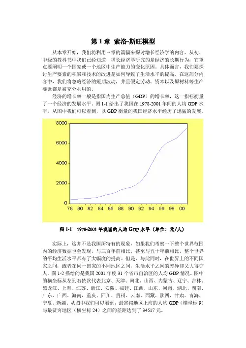
图1-1给出了我国在1978-2001年间的人均GDP水平。
从图中我们可以看到,以GDP衡量的我国经济水平经历了迅猛的发展。
图1-1 1978-2001年我国的人均GDP水平(单位:元/人)实际上,这并不是我国所特有的现象,如果我们考察一下整个世界范围内的经济数据也会发现,与三百年前相比,甚至与五十年前相比,整个世界的平均生活水平都有了大幅度的提高。
但是,与此同时,在世界上的不同国家之间,或者在同一国家的不同地区之间,生活水平之间的差异却又大得惊人。
图1-2描绘的是我国2001年度31个省市自治区的人均GDP情况。
图中的横坐标从左到右依次代表北京、天津、河北、山西、内蒙古、辽宁、吉林、黑龙江、上海、江苏、浙江、安徽、福建、江西、山东、河南、湖北、湖南、广东、广西、海南、重庆、四川、贵州、云南、西藏、陕西、甘肃、青海、宁夏、新疆。
从图中我们可以看到,最富裕地区上海的人均GDP(横坐标9)与最贫穷地区(横坐标24)之间的差距达到了34517元。
图1-2 2001年我国31个省市自治区的人均GDP(单位:元/人)单单只就上面提到的这两个事实(即在纵向上世界整体生活水平的迅速提高和在横向上各国之间或一国内的各个地区之间生活水平的巨大差异),关于经济增长研究的现实意义已不言而喻。
正如卢卡斯(Robert E. Lucas)所言:“印度政府是否可以采取一些手段来使得印度经济像印度尼西亚或埃及一样增长?如果可以,是什么手段?如果不可以,那么使得它之所以如此的印度国情究竟是什么?对于涉及于此类问题之中的人类福利而言,结果是令人惊愕的:一旦你开始考虑它们,就很难再考虑其他的事情了。
考研论坛»数学»低维拓扑knight51发表于2005-7-28 08:34低维拓扑<P>下面说说低维拓扑的内容:低维拓扑是微分拓扑的一部分,主要研究3,4维流形与纽结理论。
又叫几何拓扑。
主要以代数拓扑与微分拓扑为工具。
它与微分几何和动力系统关系密切。
国外搞这个方向的也几乎都搞微分几何和动力系统。
我国这个方向北大最牛,美国是伯克利和普林斯顿最牛。
比起代数几何来,它比较好入门。
初学者只需要代数拓扑,微分拓扑,黎曼几何的知识就行了。
美国这方面比较牛,几乎每个搞基础数学研究的都会低维拓扑。
</P><DIV class=postcolor>纠正一下上面的错误,美国也不是每个搞基础数的都精通低维拓扑,而是懂一些低维拓扑的知识。
如果入门后还想更加深入了解它,那还需要读一些双曲几何和拓扑动力系统的书。
</DIV><!-- THE POST --><!-- THE POST --><DIV class=postcolor>下面介绍一下这方面的牛人:Bill Thurston studied at New College, Sarasota, Florida. He received his B.S. from there in 1967 and moved to the University of California at Berkeley to undertake research under Morris Hirsch's and Stephen Smale's supervision. He was awarded his doctorate in 1972 for a thesis entitled Foliations of 3-manifolds which are circle bundles. This work showed the existence of compact leaves in foliations of 3-dimensional manifolds.After completing his Ph.D., Thurston spent the academic year 1972-73 at the Institute for Advanced Study at Princeton. Then, in 1973, he was appointed an assistant professor of mathematics at Massachusetts Institute of Technology. In 1974 he was appointed professor of mathematics at Princeton University.Throughout this period Thurston worked on foliations. Lawson ([5]) sums up this work:-It is evident that Thurston's contributions to the field of foliations are of considerable depth. However, what sets them apart is their marvellous originality. This is also true of his subsequent work on Teichmüller space and the theory of 3-manifolds.In [8] Wall describes Thurston's contributions which led to him being awarded a Fields Medal in 1982. In fact the1982 Fields Medals were announced at a meeting of the General Assembly of the International Mathematical Union in Warsaw in early August 1982. They were not presented until the International Congress in Warsaw which could not be held in 1982 as scheduled and was delayed until the following year. Lectures on the work of Thurston which led to his receiving the Medal were made at the 1983 International Congress. Wall, giving that address, said:-Thurston has fantastic geometric insight and vision: his ideas have completely revolutionised the study of topology in 2 and 3 dimensions, and brought about a new and fruitful interplaybetween analysis, topology and geometry.Wall [8] goes on to describe Thurston's work in more detail:-The central new idea is that a very large class of closed 3-manifolds should carry a hyperbolic structure - be the quotient of hyperbolic space by a discrete group of isometries, or equivalently, carry a metric of constant negative curvature. Although this is a natural analogue of the situation for 2-manifolds, where such a result is given by Riemann's uniformisation theorem, it is much less plausible - even counter-intuitive - in the 3-dimensional situation.Kleinian groups, which are discrete isometry groups of hyperbolic 3-space, were first studied by Poincaré and a fundamental finiteness theorem was proved by Ahlfors. Thurston's work on Kleinian groups yielded many new results and established a well known conjecture. Sullivan describes this geometrical work in [6], giving the following summary:-Thurston's results are surprising and beautiful. The method is a new level of geometrical analysis - in the sense of powerful geometrical estimation on the one hand, and spatial visualisation and imagination on the other, which are truly remarkable.Thurston's work is summarised by Wall [8]:-Thurston's work has had an enormous influence on 3-dimensional topology. This area has a strong tradition of 'bare hands' techniques and relatively little interaction with other subjects. Direct arguments remain essential, but 3-dimensional topology has now firmly rejoined the main stream of mathematics.Thurston has received many honours in addition to the Fields Medal. He held a Alfred P Sloan Foundation Fellowship in 1974-75. In 1976 his work on foliations led to his being awarded the Oswald Veblen Geometry Prize of the American Mathematical Society. In 1979 he was awarded the Alan T Waterman Award, being the second mathematician to receive such an award (the first being Fefferman in 1976).</DIV><!-- THE POST -->第2个牛人:Michael Freedman entered the University of California at Berkeley in 1968 and continued his studies at Princeton University in 1969. He was awarded a doctorate by Princeton in 1973 for his doctoral dissertation entitled Codimension-Two Surgery. His thesis supervisor was William Browder.After graduating Freedman was appointed a lecturer in the Department of Mathematics at the University of California at Berkeley. He held this post from 1973 until 1975 when he became a member of the Institute for Advanced Study at Princeton. In 1976 he was appointed as assistant professor in the Department of Mathematics at the University of California at San Diego.Freedman was promoted to associate professor at San Diego in 1979. He spent the year 1980/81 at the Institute for Advanced Study at Princeton returning to the University of California at San Diego where he was promoted to professor on 1982. He holds this post in addition to the Charles Lee Powell Chair of Mathematics which he was appointed to in 1985.Freedman was awarded a Fields Medal in 1986 for his work on the Poincaré conjecture. The Poincaré conjecture, one of the famous problems of 20th-century mathematics, asserts that a simply connected closed 3-dimensional manifold is a 3-dimensional sphere. The higher dimensional Poincaréconjecture claims that any closed n-manifold which is homotopy equivalent to the n-sphere must be the n-sphere. When n = 3 this is equivalent to the Poincaré conjecture. Smale proved the higher dimensional Poincaré conjecture in 1961 for n at least 5. Freedman proved the conjecture for n = 4 in 1982 but the original conjecture remains open.Milnor, describing Freedman's work which led to the award of a Fields Medal at the International Congress of Mathematicians in Berkeley in 1986, said:-Michael Freedman has not only proved the Poincaré hypothesis for 4-dimensional topological manifolds, thus characterising the sphere S4, but has also given us classification theorems, easy to state and to use but difficult to prove, for much more general 4-manifolds. The simple nature of his results in the topological case must be contrasted with the extreme complications which are now known to occur in the study of differentiable and piecewise linear 4-manifolds. ... Freedman's 1982 proof of the 4-dimensional Poincaré hypothesis was an extraordinary tour de force. His methods were so sharp as to actually provide a complete classification of all compact simply connected topological 4-manifolds, yielding many previously unknown examples of such manifolds, and many previously unknown homeomorphisms between known manifolds.Freedman has received many honours for his work. He was California Scientist of the Year in 1984 and, in the same year, he was made a MacArthur Foundation Fellow and also was elected to the National Academy of Sciences. In 1985 he was elected to the American Academy of Arts and Science. In addition to being awarded the Fields Medal in 1986, he also received the Veblen Prize from the American Mathematical Society in that year. The citation for the Veblen Prize reads (see [3]):-After the discovery in the early 60s of a proof for the Poincaré conjecture and other properties of simply connected manifolds of dimension greater than four, one of the biggest open problems, besides the three dimensional Poincaré conjecture, was the classification of closed simply connected four manifolds. In his paper, The topology of four-dimensional manifolds, published in the Journal of Differential Geometry (1982), Freedman solved this problem, and in particular, the four-dimensional Poincaré conjecture. The major innovation was the solution of the simply connected surgery problem by proving a homotopy theoretic condition suggested by Casson for embedding a 2-handle, i.e. a thickened disc in a four manifold with boundary.Besides these results about closed simply connected four manifolds, Freedman also proved:(a) Any four manifold properly equivalent to R4 is homeomorphic to R4; a related result holds for S3 R.(b) There is a nonsmoothable closed four manifold.© The four-dimensional Hauptvermutung is false; i.e. there are four manifolds with inequivalent combinatorial triangulations.Finally, we note that the results of the above mentioned paper, together with Donaldson's work, produced the startling example of an exotic smoothing of R4.In his reply Freedman thanked his teachers (who he said included his students) and also gave some fascinating views on mathematics [3]:-My primary interest in geometry is for the light it sheds on the topology of manifolds. Here it seems important to be open to the entire spectrum of geometry, from formal to concrete. By spectrum, I mean the variety of ways in which we can think about mathematical structures. At one extreme the intuition for problems arises almost entirely from mental pictures. At the other extreme the geometric burden is shifted to symbolic and algebraic thinking. Of course this extreme is only a middle ground from the viewpoint of algebra, which is prepared to go much further in the direction of formal operations and abandon geometric intuition altogether.In the same reply Freedman also talks about the influence mathematics can have on the world and the way that mathematicians should express their ideas:-In the nineteenth century there was a movement, of which Steiner was a principal exponent, to keep geometry pure and ward off the depredations of algebra. Today I think we feel that much of the power of mathematics comes from combining insights from seemingly distant branches of the discipline. Mathematics is not so much a collection of different subjects as a way of thinking. As such, it may be applied to any branch of knowledge. I want to applaud the efforts now being made by mathematicians to publish ideas on education, energy, economics, defence, and world peace. Experience inside mathematics shows that it isn't necessary to be an old hand in an area to make a contribution. Outside mathematics the situation is less clear, but I cannot help feeling that there, too, it is a mistake to leave important issues entirely to experts.In June 1987 Freedman was presented with the National Medal of Science at the White House by President Ronald Reagan. The following year he received the Humboldt Award and, in 1994, he received the Guggenheim Fellowship Award.<DIV class=postcolor>介绍第3个牛人:Simon Donaldson's secondary school education was at Sevenoaks School in Kent which he attended from 1970 to 1975. He then entered Pembroke College, Cambridge where he studied until 1980, receiving his B.A. in 1979. One of his tutors at Cambridge described him as a very good student but certainly not the top student in his year. Apparently he would always come to his tutorials carrying a violin case.In 1980 Donaldson began postgraduate work at Worcester College, Oxford, first under Nigel Hitchen's supervision and later under Atiyah's supervision. Atiyah writes in [2]:-In 1982, when he was a second-year graduate student, Simon Donaldson proved a result that stunned the mathematical world.This result was published by Donaldson in a paper Self-dual connections and the topology of smooth 4-manifolds which appeared in the Bulletin of the American Mathematical Society in 1983. Atiyah continues his description of Donaldson's work [2]:-Together with the important work of Michael Freedman ..., Donaldson's result implied that there are "exotic" 4-spaces, i.e. 4-dimensional differentiable manifolds which are topologically but not differentiably equivalent to the standard Euclidean 4-space R4. What makes this result so surprising is that n = 4 is the only value for which such exotic n-spaces exist. These exotic 4-spaces have the remarkable property that (unlike R4) they contain compact sets which cannot be contained inside any differentiably embedded 3-sphere !After being awarded his doctorate from Oxford in 1983, Donaldson was appointed a Junior Research Fellow at All Souls College, Oxford. He spent the academic year 1983-84 at the Institute for Advanced Study at Princeton, After returning to Oxford he was appointed Wallis Professor of Mathematics in 1985, a position he continues to hold.Donaldson has received many honours for his work. He received the Junior Whitehead Prize from the London Mathematical Society in 1985. In the following year he was elected a Fellow of the Royal Society and, also in 1986, he received a Fields Medal at the International Congress at Berkeley. In 1991 Donaldson received the Sir William Hopkins Prize from the Cambridge Philosophical Society. Then, the following year, he received the Royal Medal from the Royal Society. He also received the Crafoord Prize from the Royal Swedish Academy of Sciences in 1994:-... for his fundamental investigations in four-dimensional geometry through application of instantons, in particular his discovery of new differential invariants ...Atiyah describes the contribution which led to Donaldson's award of a Fields Medal in [2]. He sums up Donaldson's contribution:-When Donaldson produced his first few results on 4-manifolds, the ideas were so new and foreign to geometers and topologists that they merely gazed in bewildered admiration.Slowly the message has gotten across and now Donaldson's ideas are beginning to be used by others in a variety of ways. ... Donaldson has opened up an entirely new area; unexpected and mysterious phenomena about the geometry of 4-dimensions have been discovered. Moreover the methods are new and extremely subtle, using difficult nonlinear partial differential equations. On the other hand, this theory is firmly in the mainstream of mathematics, having intimate links with the past, incorporating ideas from theoretical physics, and tying in beautifully with algebraic geometry.The article [3] is very interesting and provides both a collection of reminiscences by Donaldson on how he came to make his major discoveries while a graduate student at Oxford and also a survey of areas which he has worked on in recent years. Donaldson writes in [3] that nearly all his work has all come under the headings:-(1) Differential geometry of holomorphic vector bundles.(2) Applications of gauge theory to 4-manifold topology.and he relates his contribution to that of many others in the field.Donaldson's work in summed up by R Stern in [6]:-In 1982 Simon Donaldson began a rich geometrical journey that is leading us to an exciting conclusion to this century. He has created an entirely new and exciting area of research through which much of mathematics passes and which continues to yield mysterious and unexpected phenomena about the topology and geometry of smooth 4-manifolds</DIV><DIV class=postcolor>下面continue介绍第4个牛人:Robion Kirby。
多层次logistic回归模型英文回答:Logistic regression is a popular statistical model used for binary classification tasks. It is a type of generalized linear model that uses a logistic function to model the probability of a certain event occurring. The model is trained using a dataset with labeled examples, where each example consists of a set of input features and a corresponding binary label.The logistic regression model consists of multiple layers, each containing a set of weights and biases. These weights and biases are learned during the training process, where the model adjusts them to minimize the difference between the predicted probabilities and the true labels. The layers can be thought of as a hierarchy of features, where each layer learns to represent more complex and abstract features based on the input features from the previous layer.In the context of deep learning, logistic regression can be extended to have multiple hidden layers, resulting in a multi-layer logistic regression model. Each hidden layer introduces additional non-linear transformations to the input features, allowing the model to learn more complex representations. This makes the model more powerful and capable of capturing intricate patterns in the data.To train a multi-layer logistic regression model, we typically use a technique called backpropagation. This involves computing the gradient of the loss function with respect to the model parameters and updating the parameters using gradient descent. The backpropagation algorithm efficiently calculates these gradients by propagating the errors from the output layer back to the input layer.Multi-layer logistic regression models have been successfully applied to various domains, such as image classification, natural language processing, and speech recognition. For example, in image classification, a multi-layer logistic regression model can learn to recognizedifferent objects in images by extracting hierarchical features from the pixel values.中文回答:多层次logistic回归模型是一种常用的用于二分类任务的统计模型。
磁共振3D—TOF与VIBE序列对三叉神经痛的诊断价值目的探讨磁共振三维时间飞跃法扫描序列(3D-TOF)与容积内插屏气扫描序列(VIBE序列)对三叉神经痛(trigeminal neuralgia,TN)的诊断价值。
方法在该院2012年1月—2014年10月纳入96例确诊为三叉神经痛的患者,并采用3D-TOF序列与VIBE序列大、小体素模式对患者进行扫描,记录患者三叉神经周围的血管数目,计算并分析患者的SNR(图像信号噪声比)和CNR(对比噪声比)。
结果3D-TOF序列及VIBE序列直观地呈现了原始图像中难以明确判断的血管的走向及血管压迫与患者症状的关系,96例患者中,24例患者进行了手术治疗,其中,12例患者的责任血管位于右侧小脑的上动脉,9例患者位于小脑前的下动脉,3例患者位于右侧的小脑的上动脉桥静脉及前下动脉,且三叉神经存在血管压迫或接触90例,与周围血管无压迫或接触6例,阳性率为94%,同时,经3D-TOF序列扫描显示血管的数目少于VIBE序列扫描显示的数目,VIBE序列高于3D-TOF序列。
结论联合3D-TOF序列与VIBE序列可克服两种序列的缺点,提高神经血管的成像速度并明确分辨出不同大小和血流速度的责任动脉,对三叉神经痛的诊断具有较好的临床意义。
[Abstract] Objective To discuss the value of magnetic resonance 3D-TOF sequence and VIBE sequence in diagnosis of prosopalgia. Methods 96 cases of patients with prosopalgia diagnosed in our hospital from January 2012 to October 2014 were scanned by large and small voxel models of 3D-TOF sequence and VIBE sequence,the trifacial nerve peripheral blood vessel number of the patients was recorded,the SNR (signal/noise ratio)and CNR (contrast noise ratio)of the patients were calculated and analyzed. Results The 3D-TOF sequence and VIBE sequence visually presented the vascular trend that was hard to definitely determine in the original image and the relationship between perstriction and symptoms of patients,in the 96 cases of patients,24 cases were treated with operation,among them,the offending vessel lying in anterior cerebeller artery on the right side was in 12 cases,lying in anterior inferior cerebellar artery was in 9 cases,lying in the bridging vein of anterior cerebeller artery on the right side and anterior inferior cerebellar artery was in 3 cases,perstriction or contact in trifacial nerve was in 90 cases,non-perstriction or contact with the peripheral blood vessel was in 6 cases,and the positive rate was 94%,at the same time,the blood vessel number showed by 3D-TOF sequence scanning was fewer than that showed by VIBE sequence scanning. Conclusion The 3D-TOF sequence and VIBE sequence can overcome the shortcomings of these two sequences,improve the image taking speed of nerve and blood vessel and definitely distinguish the offending vessels of different sizes and blood flow rates,and it is of better clinical significance for the diagnosis of prosopalgia.[Key words] 3D-TOF sequence;VIBE sequence;Prosopalgia;SNR;CNRTN是原发性三叉神经痛的简称,是由单条或多条责任血管压迫三叉神经的根部引起的,也是较常见的脑神经痛,其临床症状主要表现为分布区内短暂性反复发作性的刀割样或灼烧样剧痛[1]。

manifold微分流形上可以定义可微函数、切向量、切向量场、各种张量场等对象并建⽴其上的。
⼩结:1、流形(英语:Manifolds)⼀般可以通过把许多平直的⽚折弯并粘连⽽成,是局部具有性质的,是欧⼏⾥得空间中的曲线、曲⾯等概念的推⼴2、描述⼀个流形往往需要不⽌⼀个“地图”,因为⼀般来说流形并不是真正的欧⼏⾥得空间。
举例来说,地球就没法⽤⼀张平⾯的地图来合适地描绘。
微分流形(differentiable manifold),也称为光滑流形(smooth manifold),是拓扑学和⼏何学中⼀类重要的空间,是带有微分结构的拓扑流形。
微分流形是微分⼏何与微分拓扑的主要研究对象,是三维欧式空间中曲线和曲⾯概念的推⼴,可以有更⾼的维数,⽽不必有距离和度量的概念。
3-流形3-manifoldIn , a 3-manifold is a that locally looks like Euclidean 3-dimensional space. A 3-manifold can be thought of as a possible . Just as a looks like a to a small enough observer, all 3-manifolds look like our universe does to a small enough observer. This is made more precise in the definition below.The 3-dimensional torus is the product of 3 circles. That is:3维环⾯是3个圆的积流形(英语:Manifolds),是局部具有性质的,是欧⼏⾥得空间中的曲线、曲⾯等概念的推⼴。
欧⼏⾥得空间就是最简单的流形的实例。
地球表⾯这样的球⾯则是⼀个稍微复杂的例⼦。
⼀般的流形可以通过把许多平直的⽚折弯并粘连⽽成。
“manifold”这个词有多种用法。
作为形容词,它表示多种多样的,多方面的,有多种形式的,有多种用途的。
作为名词,它表示具有多种形式的东西,多支管,歧管(汽车引擎用于进气或排气)。
作为及物动词,它表示复写,复印,增多,使…多样化。
在微分几何中,manifold是一个n维空间,其局部外观像R^n。
一个n维manifold由M的每个点P的邻近的局部模型定义。
这些局部模型是R^n的开集同胚于M在P点的开集。
此外,流形中的点可能会被好几个图所表示,如果两个图重叠,它们的部分会表示流形的同一个区域。
这些部分之间的关联代表流形上同一点的坐标点的映射,称作坐标变换、变换函数或转换函数、转换映射。
以上信息仅供参考,如需了解更多信息,建议查阅英语同义词词典获取更多关于“manifold”的释义及用途。
二维Ising模型是统计物理学中的一个经典模型,它用于描述铁磁材料中的相变现象。
在该模型中,每个格点上都有一个自旋,这些自旋只能取+1或-1两个值,代表向上或向下。
自旋之间的相互作用决定了材料的宏观性质,如磁化强度。
蒙特卡洛算法是一种通过随机抽样来近似复杂系统行为的数值方法,在二维Ising模型中,蒙特卡洛算法通常指的是Metropolis-Hastings算法或其变种,用以模拟自旋系统的热力学性质。
下面将逐步介绍二维Ising模型中蒙特卡洛算法的基本思路和实现步骤。
### 1. 模型定义首先,定义二维Ising模型的哈密顿量(能量函数):### 2. 蒙特卡洛模拟步骤#### 初始化- 在\(L \times L\)的格点上随机分配自旋方向,即每个格点的自旋随机地设置为+1或-1。
#### Metropolis-Hastings算法1. **选择一个格点**:随机选取一个格点\(i\)。
2. **计算能量变化**:计算如果翻转这个格点的自旋所导致的能量变化\(\Delta E\)。
3. **接受或拒绝**:如果\(\Delta E < 0\),则接受这个变化,因为系统趋向于降低能量;如果\(\Delta E \geq 0\),则以概率\(e^{-\Delta E/k_BT}\)接受变化,其中\(k_B\)是玻尔兹曼常数,\(T\)是温度。
这一步模拟了热涨落。
4. **重复步骤**:重复上述步骤直到系统达到平衡。
#### 测量物理量- 在模拟过程中,可以测量系统的各种物理量,如磁化强度、能量、比热容等,通常需要在系统达到平衡后进行测量,并对多个蒙特卡洛步骤的结果取平均以减小统计误差。
### 3. 注意事项- **周期边界条件**:通常在模拟时使用周期边界条件来模拟无限大系统。
- **平衡时间**:系统需要足够的蒙特卡洛步骤来达到平衡,平衡时间依赖于系统大小和温度。
- **自相关时间**:为了减小测量值之间的相关性,应该在足够长的间隔后进行测量。
【德博诺的水平思考法】1. 介绍德博诺的水平思考法是一种由意大利心理学家罗伯特·德博诺提出的思考方法,这种方法旨在帮助人们更加深入地思考问题,提高思考的质量和深度。
该方法通常被用于个人和团队的决策和问题解决过程中。
2. 思维的三个维度德博诺的水平思考法主要包括三个维度:D维度(Data)、I维度(Information)和I维度(Insight)。
2.1 D维度D维度代表了数据维度,它指的是人们在思考问题时需要收集和分析的客观事实和数据。
在D维度中,人们需要通过科学的方法收集和分析数据,以便更好地了解问题的实质和本质。
对于一个问题或决策而言,D维度的数据分析可以帮助人们制定合理的决策方案。
2.2 I维度I维度代表了信息维度,它涉及到对已有知识和信息的整合和应用。
在I维度中,人们需要学会借鉴和运用已有的知识和信息,以便更好地理解问题的内在联系和规律。
通过在I维度中对信息的整合和应用,人们可以更加全面和系统地思考问题,从而得出更为深刻和准确的结论。
2.3 I维度I维度代表了洞察力维度,它要求人们在思考问题时要具备一定的洞察力和创造力。
在I维度中,人们需要超越传统的思维模式,敏锐地观察事物的本质,发现其中蕴含的新意义和新视角。
通过在I维度中培养和运用洞察力,人们可以获得更多的创新和启发,从而找到更加高效和有效的问题解决方式。
3. 应用场景德博诺的水平思考法可以应用于各种场景和领域,例如个人决策、团队问题解决、企业战略制定等。
在个人决策中,人们可以通过D维度收集和分析数据,通过I维度整合和应用信息,通过I维度发掘内在规律,从而做出更加明智和理性的决策。
在团队问题解决中,团队成员可以共同运用德博诺的水平思考法,以便更加全面和系统地思考问题,并找到更加创新和有效的解决方案。
4. 总结德博诺的水平思考法是一种适用于各种领域和场景的思考方法,它通过D维度、I维度和I维度的三个维度,帮助人们更加全面和系统地思考问题,提高了问题解决的质量和深度。
a r X i v :d g -g a /9707024v 2 5 S e p 1997FEDOSOV MANIFOLDSIsrael Gelfand(Rutgers University)igelfand@Vladimir Retakh(University of Arkansas,Fayetteville)retakh@Mikhail Shubin (Northeastern University)shubin@ Presented at Symplectic Geometry Workshop,Toronto,June 19971.Introduction.A.Connection (or parallel transport)is the main object in the geometry of mani-folds.Indeed,connections allow comparison between geometric quantities associated with different (distant)points of the manifold.In 1917Levi-Civita [Lv]introduced a notion of connection for a manifold embedded into R n .In 1918H.Weyl [We]introduced gen-eral symmetric linear connections in the tangent bundle.In 1922E.Cartan [C1],[C2],[C3]studied non-symmetric linear connections (or affine connections),where the torsion is interpreted in general relativity as the density of intrinsic angular momentum (spin)of matter.Actually Cartan explains that affine connection and linear connection with torsion is the same thing.According to Cartan,connection is a mathematical alias for an observer traveling in space-time and carrying measuring instruments.Global comparison devices (like a transformation group in the Erlangen program by F.Klein)are forbidden by the finite propagation speed restriction (see,for example,[S]).It might seem that the Riemannian geometry only requires a Riemannian metric,butthis is due to the fact that there is a canonical Levi-Civita connection associated with this metric.In this paper we study geometry of symplectic connections ,i.e.symmetric (torsion-free)connections which preserve a given symplectic form.We start (in Sect.1)with a more general context.Let us consider an almost symplectic manifold ,i.e.manifold M with a non-degenerate exterior 2-form ω(not necessarily closed)and try to describe all linear connections (i.e.connections in the tangent bundle)which preserve this form.In the classical case of non-degenerate symmetric form g =(g ij )(Riemannian or pseudo-Riemannian)the answer is well known due to Levi-Civita:for any tensor T =(T k ij ),which is antisymmetric with respect to the subscripts i,j ,there existsa unique connection Γ=(Γk ij )with the torsion tensor T (i.e.Γk ij −Γk ji =T k ij )such thatΓpreserves g .If T =0,this connection is called the Levi-Civita connection .It is the canonical connection associated with g .Wefirst prove a skew-symmetric analog of this Levi-Civita ly,there is a canonical one-one correspondence between the following two sets of linear connections on an almost symplectic manifold(M,ω):1)all symmetric connections on M;2)all connections on M which preserveω.This correspondence is obtained as follows:for a connectionΓwhich preservesω,we just take its symmetric partΠ=(Πi jk),Πi jk=1of unity.Therefore a structure of a symplectic manifold can be always extended to a structure of a Fedosov manifold.In fact the symplectic connections on a symplectic manifold form an infinite-dimen-sional affine space with difference vector-space isomorphic to the space of all completely symmetric3-covariant tensors-see e.g.[BFFLS],[Ve]and Section1(the paragraph after (1.5))below.Fedosov manifolds constitute a natural generalization of K¨a hler manifolds.A K¨a hler manifold can be defined as a Riemannian almost complex manifold(M,g,J)(here g is a Riemannian metric and J an almost complex structure on the manifold M),such that J is orthogonal with respect to g and parallel with respect to the Levi-Civita connectionΓassociated with g(see e.g.[K-N],vol.2,Ch.IX,Sect.4,or[Br],p.148).The last property can be formulated by saying that the2-formωdefined by g,J according to the formula (0.1)ω(X,Y)=g(X,JY),isΓ-parallel,i.e.invariant under the parallel transport defined byΓ(or,equivalently,its covariant derivative vanishes).It follows thatωis closed,hence symplectic because it is automatically non-degenerate.Therefore every K¨a hler manifold is a Fedosov manifold.On the other hand there are symplectic manifolds such that they do not admit any K¨a hler structure,even with a differentω(see e.g.[Br],p.147,for a Thurston example).We study the curvature tensor of a symplectic connection(on a Fedosov manifold). The usual curvature tensor R i jkl is well defined by the connection alone.But the tensorR ijkl=ωip R pjkl is more interesting.(We use the standard Einstein summation convention,so here the summation over p is understood.)This tensor is well known.For example, V.G.Lemlein[Lm]introduced it in a more general context of almost symplectic manifolds with a connection,I.Vaisman[Va1]obtained important symmetry properties.Since we tried to make this paper self-contained,we give(usually new)proofs of some properties of this tensor which werefirst obtained in[Va1].Following I.Vaisman we will call R ijkl the symplectic curvature tensor.The symplectic curvature tensor has symmetries which are different from the sym-metries of the curvature tensor on a Riemannian ly,aside of standard symmetries R ijkl=−R ijlk,R i(ijk)=0(here the parentheses mean that we should take sum over all cyclic permutations of the subscripts inside the parentheses),it is symmetric with respect to thefirst two subscripts:R ijkl=R jikl.We deduce from these identities that R(ijkl)=0.C.In Sect.3we consider the Ricci tensor K ij=R k ikj=ωkp R pikj which is again defined by the connection alone.I.Vaisman[Va1]proved that it is in fact symmetric(as in the case of Riemannian manifolds)and the structure of the Fedosov manifold plays important role in the proof.We give two proofs of the symmetry of K ij(in particular we deduce it from the identity R(ijkl)=0).There are two natural non-trivial contractions of the curvature tensor on a Fedosov manifold seemingly leading to two different Ricci type tensors(tensors of type(2,0)orbilinear forms on each tangent space).However we prove that they only differ by a constant factor2:ωkl R ijkl=2K ij.We also prove that the operatorL=ωij∇i∇j,on vectorfields has order zero and corresponds to the Ricci tensor(with one subscriptlifted byω).In the Riemannian case contracting the Ricci tensor we obtain the scalar curvature. On a Fedosov manifold we can only use the symplectic form for the contraction,and thisobviously leads to a trivial result.Note also that I.Vaisman[Va1]provided a complete group-theoretic analysis of the space of all curvature-type tensors(i.e.tensors with the symmetries described above)asa representation space of the group Sp(2n),where2n=dim R M.He proved that the corresponding representation space splits into a direct sum of two suspaces,one of them isthe space of all tensors with vanishing Ricci curvature part,and another is also explicitly described.Each of these two subspaces is irreducible.Vanishing of the Ricci tensor provides the vacuum Einstein equations in the Rieman-nian or pseudo-Riemannian case.This is a determined system for the components of the metric.We can also write the vacuum Einstein equations K ij=0on a Fedosov manifold. We call the manifolds with this property symplectic Einstein manifolds.(They are called Ricciflat in[Va1].)However K ij=0is an undetermined system(for the symplectic form together with the symplectic connection).The obvious local gauge transformations(sym-plectic transformations of coordinates)are not sufficient to remove the underdeterminacy even in dimension2.We also give a definition of sectional curvature on a Fedosov manifold.It is a function on non-isotropic2-planesΠin the tangent bundle,and it is defined by the canonical form of the quadratic form Z→R(Z,Z,X,Y),Z∈Π,where{X,Y}is a basis ofΠsuch that ω(X,Y)=1.The quadratic form may be degenerate of rank0or1.If it is non-degenerate, then it has a real(non-zero)invariant and can also be elliptic or hyperbolic.D.In Sect.4we introduce normal coordinates on a Fedosov manifold.They are defined as affine coordinates in the tangent space to T p M which are transferred to M by the exponential map of the given connectionΓat p.Since they are defined by the connection only,the construction does not differ from the Riemannian case.We can also define affineextensions of an arbitrary tensor T=(T i1...i kj1...j l )which are tensors T i1...i kj1...j lα1...αrobtainedat p∈M by taking the corresponding derivatives of the components of T in normal coordinates centered at p and then evaluating the result at p.Applying this procedure to the Christoffel symbolsΓijk,we obtain so called normal tensorsA ijk=0,A ijkα1,A ijkα1α2,....(They are tensors in spite of the fact thatΓijk do not form a tensor,and due to the fact thatΓijk undergo the tensor transformation law if the transformation of the coordinates is linear.)Extending results of T.Y.Thomas and O.Veblen(see e.g.[E,Th,V])we describe all algebraic relations for the normal tensors and the extensions of the symplectic form at a point of a Fedosov pared with the classical situation(arbitrary symmetric connection)a new relation is added to provide the compatibility of the normal tensors with the existence of the preserved symplectic form(see(4.18)).We also prove that all local invariants of a Fedosov manifold are appropriate functions of the components of the normal tensors and of the components of the symplectic form.E.In Section5we study relations between the normal tensors and the curvature ten-sor.Here we again use an appropriately modified technique by T.Y.Thomas and O.Veblen. We provide formulas which express normal tensors through the extensions of the curvature tensor(or its covariant derivatives)and vice versa.A simplest corollary of these formulas is1ωij,kl=Let∇be a connection(covariant derivative)on M.We will say that∇preservesωif ∇ω=0or(1.1)Z(ω(X,Y))=ω(∇Z X,Y)+ω(X,∇Z Y)for any vectorfields X,Y,Z.Let us write this in coordinates.If x1,...,x n are local coordinates,denote∂i=∂(Γk ij+Γk ji).2Theorem1.1.The mapΓ→Π(Γ)gives a bijective affine correspondence between the set of all connections preservingωand the set of all symmetric connections.The inverse mapΠ→Γis given by1(1.7)Γkij=Remark1.5.Suppose we are given non-degenerate symmetric and antisymmetric 2-forms g andωat the same time.Then we can construct a sequence of connections. Let us start with any antisymmetric torsion tensor T0(e.g.zero).Then there exists a unique g-preserving connectionΠg1with the torsion T0.Denote by S1its symmetric part (this is a symmetric connection).Then we canfind a(unique)ω-preserving connectionΓω1 which has the symmetric part S1.Denote its torsion tensor by T1.Now we can repeat the construction starting with T1instead of T0.In this way we obtain a sequence of connections and torsion tensorsT0→Πg1→S1→Γω1→T1→Πg2→S2→Γω2→T2→....This sequence looks similar to the sequence which appears when one uses two symplectic structures in the theory of integrable systems.Note that for K¨a hler manifolds,starting with T0=0we obtain the sequence which stabilizes i.e.we get T j=0,Πg j=S j=Γωj for all j.Remark1.6.Independently of Theorem1.1it is easy to observe a coincidence of functional dimensions(the number of independent functional parameters)of the two sets of connections above:all connections preservingωand all symmetric connections.Playing with the dimensions we noticed another curious coincidence:(1.9)C n−Cωn=S n−Sωn+Λ3n,whereωis a given non-degenerate(exterior)2-form,C n=f-dim of all connections=n3,(f-dim means functional dimension)(n+2)(n+1)n Sωn=f-dim of symmetric connections preservingω=,2n2(n+1)S n=f-dim of all symmetric connections=.6It would be interesting to clarify the coincidence(1.9)(similarly to the clarification of the “coincidence”Cωn=S n which was given above).2.Symplectic connections and their curvature.Let(M,ω)be a symplectic manifold,∇(orΓ)a connection on M.Definition2.1.If∇is symmetric and preserves the given symplectic formωthen we will say that∇is a symplectic connection.Definition2.2.Fedosov manifold is a symplectic manifold with a given symplectic connection.A Fedosov manifold(M,ω,Γ)is called real-analytic if M,ω,Γare all real-analytic.The curvature tensor of a symplectic connection is defined by the usual formula (2.1)R(X,Y)Z=∇X∇Y Z−∇Y∇X Z−∇[X,Y]Z.The components of the curvature tensor are introduced by(2.2)R(∂j,∂k)∂i=R m ijk∂m.Denote also(2.3)R ijkl=ωim R m jkl=ω(∂i,R(∂k,∂l)∂j).Instead of R ijkl we can also consider R(X,Y,Z,W)which is a multilinear function on any tangent space T x M(or a function of4vectorfields which is multilinear over C∞(M)): (2.3′)R(X,Y,Z,W)=ω(X,R(Z,W)Y),so that R ijkl=R(∂i,∂j,∂k,∂l).But it is usually more convenient to do calculations using components.It is obvious that(2.4)R ijkl=−R ijlk.The formula expressing the components of the curvature tensor in terms of the Christoffel symbols has the standard form:(2.5)R l ijk=∂jΓl ki−∂kΓl ij+Γm kiΓl jm−Γm ijΓl km.For any symmetric connection we have thefirst Bianchi identity(2.6)R i(jkl):=R ijkl+R iklj+R iljk=0.(For the proofs of(2.5)and(2.6)see e.g.[D-F-N],Sect.30,or[He],Ch.1,Sect.8,12).Proposition2.3.[Va1]For any symplectic connection(2.7)R ijkl=R jikl.Proof.Let us consider(2.8)∂k∂lωij=∂k[ω(∇l∂i,∂j)+ω(∂i,∇l∂j)]==ω(∇k∇l∂i,∂j)+ω(∇l∂i,∇k∂j)+ω(∇k∂i,∇l∂j)+ω(∂i,∇k∇l∂j). Changing places of k,l and subtracting the result from the(2.8)we obtain: 0=ω([∇k,∇l]∂i,∂j)+ω(∂i,[∇k,∇l]∂j)=ω(R m ikl∂m,∂j)+ω(∂i,R m jkl∂m)==ωmj R m ikl+ωim R m jkl=−R jikl+R ijkl.Proposition2.4.For any symplectic connection(2.9)R(ijkl):=R ijkl+R lijk+R klij+R jkli=0.ing(2.6)we obtainR ijkl+R iklj+R iljk=0,R jikl+R jkli+R jlik=0,R kijl+R kjli+R klij=0,R lijk+R ljki+R lkij=0.Adding all these equalities and using(2.4)and(2.7),we obtain(2.9).3.Ricci tensor and sectional curvature.Let us look for possible contractions of the curvature tensor which can lead to new non-trivial tensors.Lemma3.1.On any Fedosov manifold(3.1)R k kij=ωkl R lkij=0.Proof.The result immediately follows from the symmetry of R lkij with respect to thefirst two subscripts(Proposition2.3).Definition3.2.The Ricci tensor of a Fedosov manifold is defined by the formula (3.2)K ij=R k ikj=ωkl R likj.Equivalently we can define K as a bilinear form on T x M:(3.2′)K(X,Y)=K ij X i Y j=tr{Z→R(Z,Y)X},where X,Y,Z∈T x M,X=X i∂i,Y=Y j∂j.Note that the Ricci tensor depends on connection only.(It does not depend onω.)Proposition3.3.[Va1]On any Fedosov manifold the Ricci tensor is symmetric: (3.3)K ij=K ji.Proof.Multiplying(2.9)byωki,summing over k,i and using the symmetries(2.4) and(2.7)of the curvature tensor we get the desired result.Corollary3.4.[Va1]On any Fedosov manifold(3.4)ωji K ij=0.This means that the usual way to define the scalar curvature gives a trivial result.Now let us show that the second non-trivial contraction of the curvature tensor again leads to the Ricci tensor.Proposition3.5.On any Fedosov manifold(3.5)ωkl R ijkl=2K ij.ing(2.6)and the symmetries(2.4),(2.7),we obtainωkl R ijkl=ωkl(−R iklj−R iljk)=ωlk R kilj+ωkl R likj=2K ij.Remark3.6.Since the left hand side of(3.5)is symmetric in i,j due to the symmetry (2.7),the formula(3.5)provides another proof of the symmetry of the Ricci tensor.Yet another definition of the Ricci tensor can be extracted from the followingProposition3.7.Denote(3.6)L=ωij∇i∇j,which is considered as an operator on vectorfields.Then L in fact has order0and (3.7)(LX)i=L i j X j,L i j=ωik K kj,so(3.8)K ij=ωik L k j.or on other words(3.8′)K(X,Y)=ω(X,LY),X,Y∈T x M.Proof.We haveL=ωij∇i∇j=12ωij R(∂i,∂j),therefore(LX)i=12ωiqωkl R qpkl X p=ωiq K qp X p,where we used Proposition3.5.Now(3.7),(3.8)and(3.8’)immediately follow.The following definition is a possibility to introduce an analogue of the Einstein equa-tions on a Fedosov manifold.Definition3.8.Einstein equation on a Fedosov manifold is the system(3.9)K ij=0.This is a system of nonlinear equations on the data of the Fedosov manifold:its symplectic form and connection.There is an important difference with the symmetric case:the system (3.9)is not determined.Indeed,using Darboux coordinates we can assume thatωhas a canonical form and we only seek the Christoffel symbolsΓijk which should be completely symmetric(see Sect.1).It is easy to see that the functional dimension(the number of free functional parameters)for the space of such connections is(n+2)(n+1)n/6(here n=dim R M),whereas for the space of symmetric2-tensors it is(n+1)n/2.The equality of these functional dimensions holds if and only if n=1,which can not be a dimension of a Fedosov manifold.On the other hand the equation(3.9)is non-trivial.Indeed,using(2.5)we obtain in Darboux coordinates(3.10)R likj=∂kΓlji−∂jΓlik+ωmpΓpjiΓlkm−ωmpΓpikΓljm,therefore(3.11)K ij=ωkl R likj=ωkl∂kΓlij−ωklωmpΓpikΓljm,because after multiplication byωkl and summation over k,l the second and he third terms in(3.10)vanish due to the symmetry ofΓijk in i,j,k.Definition3.9.Symplectic Einstein manifold is a Fedosov manifold such that its Ricci tensor vanishes,i.e.the Einstein equation(3.9)is satisfied.In terminology of I.Vaisman[Va1]such manifolds are called Ricciflat.Let us discuss a possibility to define sectional curvature.Consider a2-dimensional subspaceΠin a tangent space T x M to a Fedosov manifold M at a point x∈M.For any X,Y∈Πconsider a quadratic form onΠgiven by(3.12)E X,Y(Z)=R(Z,Z,X,Y).Assuming thatΠis symplectically non-degenerated(non-isotropic)we can choose X,Y so thatω(X,Y)=1and E X,Y has one of the following forms:(3.13)E X,Y(Z)=r(Z21+Z22),r∈R\{0};(3.14)E X,Y(Z)=r(Z21−Z22),r>0;(3.15)E X,Y(Z)=Z21,(3.16)E X,Y(Z)=0,where Z1,Z2are coordinates of Z in the basis X,Y.Here r=r(Π)does not depend on the choice of the basis X,Y inΠ.Note thatω(X,Y)=1implies that the determinant of the matrix of the form E X,Y in the basis X,Y does not depend on X,Y and equals r2 and−r2in the cases(3.13)and(3.14)respectively,and0in the cases(3.15)and(3.16). Define also r(Π)=0in the cases(3.15)and(3.16).The canonical form of E X,Y is defined as the choice of one of the possibilities(3.13)–(3.16)together with an extra parameter r in cases(3.13)and(3.14)(real non-zero or positive respectively).We will refer to the case(3.13)as elliptic,(3.14)as hyperbolic, (3.15)as degenerate and(3.16)asflat.Definition3.10.Sectional curvature of a Fedosov manifold M is a functionΠ→{canonical form of E X,Y}In particular we have a continuous functionΠ→r(Π)which is defined on the set of all symplectically non-degenerated(non-isotropic)2-dimensional subspacesΠin the tangent bundle T M.This function may become singular when we approach the subset of all isotropic planes in the Grassmanian bundle of all2-planes in T M.Example3.11.Consider the2-sphere S2R of the radius R in R3with the structure of a Fedosov manifold such that the connection is induced by the parallel transport in R3 (or,equivalently,is the Levi-Civita connection of the Riemannian metric induced by the canonical metric in R3)and the symplectic form is given by the area(induced by the same Riemannian metric).Then a straightforward calculation shows that all tangent planes are elliptic with r(Π)identically equal to1/R2.Example3.12.Consider the standard Lobachevsky(or hyperbolic)plane H2,e.g. the half-plane model{(x,y)∈R2|y>0}with the Riemannian metricdx2+dy2ds2=which we will denote˜R ijkl=g(∂i,R(∂k,∂l)∂j)and the curvature of M as a Fedosov manifold(we will denote it R ijkl as above).There is an obvious relation between them: (3.17)˜R ijkl=g ip R pjkl=g ipωpm R mjkl.We can write this relation in a different form using the complex structure J from(0.1) (see[Va1]):(3.17′)˜R(X,Y,Z,W)=R(JX,Y,Z,W).Indeed,˜R(X,Y,Z,W)=g(X,R(Z,W)Y)=ω(JX,R(Z,W)Y)=R(JX,Y,Z,W).4.Normal coordinates and extensions.Let us consider a manifold M with a given non-degenerate2-formω.LetΓbe a symmetric connection on M.(At the moment we do not assume thatΓpreservesω.) Given a point p∈M we have the exponential map exp p:U→M defined byΓ.Here U is a small neighborhood of0in T p M,and exp p(v)=x(1)where v∈U and x(t)is a geodesic defined in local coordinates(x1,...,x n)near p by(4.1)d2x idtdx k∂x j(p)=δi j.In this case(y1,...,y n)are called the normal coordinates associated with the local coordi-nates(x1,...,x n)at p.In other words,ifξ=y1∂∂x n ∈T p M then(y1,...,y n)are the normalcoordinates of exp pξ.Normal coordinates are actually defined by the connection(they do not depend on the formω).We will list several properties of the normal coordinates(see e.g.[E],[T], [V]).Let(y1,...,y n)be local coordinates such that a given point p∈M corresponds to y1=...=y n=0.Then they are normal coordinates if and only if(4.3)Γi jk(y)y j y k≡0,whereΓi jk(y)are the Christoffel symbols which are calculated at a point with the local coordinates y=(y1,...,y n)in the coordinates y j.Usingωwe can pull the superscript i down and rewrite(4.3)equivalently in the form (4.4)Γijk(y)y j y k≡0.Taking y j=tξj in(4.4),dividing by t2and taking the limit as t→0,we obtain due to the symmetry ofΓijk in j,k:(4.5)Γijk(0)=0.Let us write the Taylor expansion ofΓijk at y=0in the form:(4.6)Γijk(y)=∞r=11∂yα1...∂yαry=0.Here p∈M is the“origin”of the normal coordinates.Note that different normal coordinates with the same origin differ by a linear trans-formation.It follows that the correspondence p→A ijkα1...αr (p)defines a tensor on M(the components should be related to our start-up coordinate system(x1,...,x n)).Definition4.1.The tensor A ijkα1...αr is called an affine normal tensor or an affineextension ofΓijk of order r=1,2,....We also take by definition A ijk=0which is natural due to(4.5).Proposition4.2.The affine normal tensors have the following properties:(i)A ijkα1...αr is symmetric in j,k and also inα1,...,αr(i.e.with respect to thetransposition of j and k and also with respect to all permutations ofα1,...,αr;(ii)for any r=1,2...(4.8)S j,k֒→j,k,α1,...,αr (A ijkα1...αr)=0,where S j,k֒→j,k,α1,...,αr stands for the sum of all the(r+2)(r+1)/2terms obtainablefrom the one written within parentheses by replacing the pair j,k by any pair from the set {j,k,α1,...,αr}.(iii)Assume that a non-degenerate2-formωon M isfixed.If the tensors{A ijkα1...αr |r=1,2,...}are given at one point p,satisfy the conditions in(i),(ii)and be-sides the series(4.6)is convergent in a neighborhood of0,then the sums in(4.6)constitute the set of the Christoffel symbols of a symmetric connection in normal coordinates.The proof easily follows from(4.4)and it does not differ from the proof of the version of this statement forΓi jk which is given e.g.in[E],[T],[V].It can be also reduced to the corresponding statement forΓi jk by pulling down the superscript i.Examples of the identity(4.8)for r=1and r=2are as follows:(4.9)A ijkl+A ijlk+A iklj=0;(4.10)A ijklm+A ijlkm+A ijmkl+A ikljm+A ikmjl+A ilmjk=0.Let us consider an arbitrary tensor T=(T i1...i kj1...j l)on M.Definition4.3.The(affine)extension of T of order r is a tensor on M,such that its components at the point p∈M in the local coordinates(x1,...,x n)are given by the formulas(4.11)T i1...i kj1...j l,α1...αr =∂r T i1...i kj1...j lr!ωij,α1...αr(0)yα1...yαr.It follows that∂kωij=∂r!ωij,α1...αr(0)rs=1yα1...δαsk...yαr=∞r=11(r−1)!ωij,kα1...αr−1(0)yα1......yαr−1or(4.15)∂kωij(y)=∞ r=01(f)the series(4.6)and(4.14)are convergent for small y.The structure of a real-analytic Fedosov manifold near0is uniquely defined by the tensors (4.16).2)Assume that we are only given tensors A ijkα1...αr (0)such that the conditions(a),(b)are satisfied and the series(4.6)is convergent for small y.Then a real-analytic symplectic form near0complementing the connection(defined byΓijk given by the series(4.6))to a local real-analytic Fedosov manifold structure near0exists if and only if for all r=1,2,...(4.18)A ikjα1...αr (0)−A jkiα1...αr(0)is symmetric in k,α1,i.e.with respect to the transposition of k andα1.The formωabove is uniquely defined by ωij(0)and it exists for arbitrary skew-symmetric non-degenerateωij(0).Proof.1)It is obvious from the considerations above that the conditions(a)-(f)are necessary for the existence of a local real-analytic Fedosov manifold near0with the given extensions(4.16).They are also sufficient because we can defineωij(y)andΓijk(y)near0 by the convergent series(4.6)and(4.14),and it is easy to see that all the conditions will be satisfied.The uniqueness ofω,Γnear0is obvious because the tensors(4.16)define all the Taylor coefficients ofω,Γat0.2)If the tensors A ijkα1...αr satisfy(a),(b)and the series(4.6)are convergent forsmall y,then the sums of these series provideΓijk(y)which determine a real-analytic symmetric connection in normal coordinates for any given real-analytic non-degenerate skew-symmetric formωij(y)defined near0.To make this2-form symplectic and preserved byΓwe can try tofind it from the conditions(4.13)which determine allfirst derivatives ∂kωij near0,so we only need to knowωij(0).Let us choose an arbitrary skew-symmetric matrixωij(0).Then we canfindωij(y) from(4.13)if and only if the following compatibility conditions are satisfied near0: (4.19)∂l(Γikj−Γjki)=∂k(Γilj−Γjli),or,equivalently,(4.20)∂l(Γikj−Γjki)is symmetric in k,l.But the same argument as the one leading to(4.15),shows that the Taylor expansion of ∂lΓikj(y)at0has the form(4.21)∂lΓikj(y)=∞ r=11(with arbitrary constant skew-symmetric non-degenerateωij),if and only if A ijkα1...αr aresymmetric in i,j,k and inα1,...,αr,and besides the conditions(4.8)are satisfied.Proof.Let usfix an arbitrary constant skew-symmetric non-degenerateωij.The condition(4.8)guarantees that the sumsΓijk(y)of the series(4.6)give us components of a symmetric connection in normal coordinates due to Proposition4.2.Now(1.2)implies that this connection preserves the constant formωif and only ifΓijk is symmetric in ijk which is equivalent to saying that A ijkα1...αrare symmetric in i,j,k for any r=1,2,....Now we can formulate the simplest result about local invariants of Fedosov manifolds. For simplicity we will only consider invariants which are tensors though similar results are true e.g.for invariants which are tensors with values in density bundles.Definition4.7.A tensor T=(T i1...i kj1...j l (x))on a Fedosov manifold M is called a localinvariant of M if its components at each point p∈M are functions of afinite number of derivatives(of arbitrary order,including0)ofΓijk andωij taken at the same point p in local coordinates,i.e.(4.22)T i1...i kj1...j l (p)=F i1...i kj1...j l(Γijk(p),∂αΓijk(p),...,ωij(p),∂αωij(p),∂α2∂α1ωij(p),...),where the functions F i1...i kj1...j ldo not depend on the choice of the local coordinates.Alocal invariant is called rational or polynomial if the functions F i1...i kj1...j l are all rational orpolynomial respectively.In particular,this definition applies to local invariants which are differential forms.Theorem4.8.Any local invariant of a Fedosov manifold is a function ofωij and a finite number of its affine normal tensors,i.e.it can be presented in the form(4.23)T i1...i kj1...j l (p)=G i1...i kj1...j l(ωij(p),A ijkα1(p),...,A ijkα1...αr(p)),where the functions G i1...i kj1...j ldo not depend on the choice of local coordinates.If the invariantT i1...i k j1...j l is rational or polynomial,then the functions G i1...i kj1...j lare also rational or polynomialrespectively.Proof.Since T is a tensor,its components T i1...i kj1...j l(p)will not change if we replace local coordinates(x1,...,x n)by normal coordinates(y1,...,y n)which are associated with (x1,...,x n)at p.But then according to Definition4.7we obtain,using formulas(4.7)and (4.12):(4.24)T i1...i kj1...j l (p)=F i1...i kj1...j l(0,A ijkα(p),...,ωij(p),0,A iα1jα2(p)−A jα1iα2(p),...).All statements of the Theorem immediately follow.5.Normal tensors and curvature.。