10 DOF IMU Sensor (D)

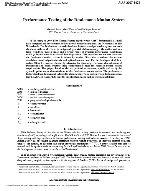
AIAA Modeling and Simulation Technologies Conference and Exhibit 20 - 23 August 2007, Hilton Head, South CarolinaAIAA 2007-6472Performance Testing of the Desdemona Motion SystemManfred Roza1, Mark Wentink2 and Philippus Feenstra3 TNO Human Factors, Soesterberg, The NetherlandsTP PT TP PT TP PTIn the spring of 2007 TNO Human Factors together with AMST Systemtechnik GmbH have completed the development of their newest research simulator, the Desdemona, in The Netherlands. The Desdemona research simulator features a unique motion system not seen elsewhere in the world. Its serial design and geometrical dimensions give the motion system a large cylindrical motion space and a broad range of dynamic performance capabilities, which go beyond those of a classical Stewart platform. Like any other motion-base simulator the Desdemona motion system is driven by motion filters that transform the various simulation model outputs into safe and optimal motion cues. For the development of these motion filters it is necessary to exactly determine the dynamic performance characteristics of Desdemona and check whether these characteristics meet the specified motion system requirements. This paper describes the test protocol to measure, specify and verify the dynamic performance characteristics of the Desdemona motion system. The performance test protocol builds upon and extends the classical synergistic motion system test approaches, like the AGARD standard, to suite the specific Desdemona motion system capabilities.NomenclatureM&S DOF IMU MCC PLC = = = = = = modeling and simulation degree of freedom inertial measurement unit motion control computer programmable logical controller central yaw axisψ centrR Hφcab ψ cab θ cab= radial axis = heave axis = cabin roll axis = cabin yaw axis = cabin pitch axisI. IntroductionTNO Defense, Safety & Security in the Netherlands has a long tradition in research into modeling and simulation (M&S) technology and applications. The M&S effort of TNO Human Factors is centered in the area of flight, driving and ship simulators for human performance, training and behavior research. Over the years TNO Human Factors has specialized in human perception research ranging from visual & vestibular research to motion sickness and fidelity, to 3D-audio and haptic interfacing experiments1,4,5,6,7,8,9. To better facilitate this kind of research and the spatial disorientation training for the Royal Netherlands Air Force, TNO Human Factors initiated the development of a new research simulator, the Desdemona11,12,13.P P P PIn co-operation with AMST Systemtechnik GmbH, TNO Human Factors completed the development of the Desdemona simulator, in the late spring of 2007. The Desdemona research simulator features a unique and special designed non-synergistic motion system with six degrees of freedom (DOF). Its serial design and geometrical1TPResearch Scientist, TNO Defence, Safety & Security, Human Factors Department, manfred.roza@tno.nl, AIAA Member. Research Scientist, TNO Defence, Safety & Security, Human Factors Department, mark.wentink@tno.nl, AIAA Member. 3 Research Scientist, TNO Defence, Safety & Security, Human Factors Department, philippus.feenstra@tno.nl.PT HTU UTH2TP TPPTHTUUTHPTHTUUTH1 American Institute of Aeronautics and AstronauticsCopyright © 2007 by the American Institute of Aeronautics and Astronautics, Inc. All rights reserved.dimensions give the motion system a large cylindrical motion space and a broad range of dynamic performance capabilities. One of the unique motion capabilities is the ability to combine onset cueing like a classical Stewart or hexapod platform with sustained acceleration cueing as found in dynamic flight simulators. Furthermore, the rotating gimbal system gives the Desdemona motion system the possibility to replicate unusual attitudes and large attitude changes one-to-one. The motion system houses a cabin, which is equipped with a 120 degree visual system. The modular hard and software design of the cabin enables fast reconfiguration of the interior and the installation of human machine interfaces. This makes the Desdemona simulator potentially suitable for a wide range of research applications including unusual aircraft and rotorcraft maneuvers, suburban, urban and terrain driving simulation, motion perception and cueing, spatial disorientation, motion sickness, and human-performance in artificial gravity conditions.Figure 1. The Desdemona Research Simulator Exterior Like all other motion-base simulators the Desdemona motion system is driven by motion filters that transform the various simulation model outputs into safe and optimal motion cues 13, 14. For the development of these motion filters it is necessary to exactly determine the Desdemona dynamic performance characteristics. In addition, the measured performance is used to verify whether it meets the specified motion system requirements. This paper describes the test protocol to measure, specify and verify the dynamic performance characteristics of the Desdemona motion system. The paper starts in Section II with a presentation of the Desdemona motion system configuration and properties. Next the rationale and top-level design of the dynamic motion test protocol are discussed (Section III). This protocol builds upon and extends the classical synergistic motion system test approaches described in literature such as AGARD and ASC/MIL standards to suite the specific Desdemona motion system capabilities 15,16. In two subsequent sections the various tests and associated performance metrics of the protocol are discussed. These tests are divided in two categories. The first category is the single axis tests (Section IV). These tests comprise timedomain tests for motion system position, velocity and acceleration limits and signal tracking accuracy, and frequency domain system identification based tests. Multi-axis performance tests form the second category of tests (Section V). These tests are typical for serial motion systems, like the Desdemona, where independent axes have to be moved in conjunction to reproduce the desired motion cues during simulation. Lessons-learned and experiences from the first execution of the Desdemona motion performance test protocol are presented in Section VI. The paper ends in Section VII with conclusions and future work to motion system performance testing in relation to research into motion system fidelity, perception and requirements.2 American Institute of Aeronautics and AstronauticsII. Desdemona Motion System DescriptionA. Motion System Configuration and Characteristics Unlike conventional motion systems such as the Stewart platform, the Desdemona motion system is not a synergistic or parallel robotic system. Instead the Desdemona has a non-synergistic or a serial motion system with six axes that can be moved independently (Figure 2). These six axes are respectively called: central yaw (ψ centr ), radius (R), heave (H), cabin roll ( φcab ), cabin yaw (ψ cab ) and cabin pitch ( θ cab ). The Desdemona cabin is suspended in a fully gimbaled 3DoF system ( φcab ,ψ cab and θ cab ), which allows unlimited cabinrotation around any arbitrary axis in space. This gimbaled system is mounted in a heave system (H) that translates the gimbal system and the cabin in the vertical plane. The heave/gimbal system can be moved horizontally over a sledge; the radius (R). The sledge itself can be rotated unlimited in the middle around a vertical axis (ψ centr ); the central yaw axis. This central yaw axis in combination with the radius gives the Desdemona motion system the capability of sustained g-load generation up to 3g.Figure 2. The Desdemona Motion System DOFAll the axes are driven by electric servo-systems. The required performance characteristics for each of these Desdemona axes in terms of the maximum attainable position, velocity and acceleration are given in the table below.Central Yaw Max. position Max. Velocity Max. Acceleration Radius Heave Cabin Roll Cabin Yaw Cabin Pitch>360P0P±4m 3.2 m/s 4.9 m/s2P±1m 2.0 m/s 4.9 m/s2>360P0P>360P0P>3600P P155 /sP P0180 /sP P0180 /sP P0180 /sP P045 /sP P P0290 /sP P P02P90 /sP P P02P90 /s2P P P P0Table 1 Maximum Position, Velocity and Acceleration Characteristics of the Desdemona Motion System B. Motion Control, Measurement and Integrated Test Systems The Desdemona motion platform is controlled by a motion control computer (MCC), which runs on a standard PC with a real-time operating system. The MCC hosts all necessary control logic, safety and communication I/O software to safely operate the Desdemona motion system. An Ethernet network with a dedicated protocol is used for the communication between the MCC and several PLC’s. These PLC’s form the interface between the MCC and the peripheral motion system hardware such as the engine drives, measurement and safety systems, and various analogue and digital I/O. A CanOpen field bus is used for communication and data transport between the drive PLC’s and the engine drives. The MCC software architecture allows for both running the , e.g. vehicle model and motion filter on the MCC itself or remotely on different PC’s in a distributed simulator architecture design. This gives the Desdemona simulator additional flexibility in developing and off-line testing of vehicle model and motion filter configurations. The MCC operates and generates motion control reference signals at a rate of 200Hz. The Desdemona motion system is equipped with three types of measurement systems, which could be used for dynamic performance testing. The first measurement system comprises the various position encoders mounted on each axis, which are used by the electrical drives to control each axis position. The second measurement system comprises three solid state accelerometers mounted on the cabin chair at the position of the subjects head. These 3 American Institute of Aeronautics and Astronauticsthree sensors are intended for safety purposes to measure the local specific force vector exerted on the subject7. The last measurement system is an Inertial Measurement Unit (IMU), which comprises a fiber-optics and temperature compensated 3-axis gyro in combination with a solid-state 3-axis accelerometer. These high quality sensors have specifically been selected for motion performance measurement purposes. The gyro is rigidly attached to the inside of the cabin structure and the accelerometer is also attached to the cabin but with a flexible mechanical connection. This provides digital output signals of the three cabin (mechanical low-pass filtered) accelerations and the angular rates. All measurement systems are connected to the Desdemona integrated test system. This test system is capable of injecting test-signals, logging and visualizing all the actual sensor data at a rate of 200Hz. C. Post processing of measurement data: filtering and differentiating The motion performance measurement and analysis of Desdemona comprises the orientation or positions of each degree of freedom and their first and second order derivatives. However, not all derivatives are directly measured by the aforementioned Desdemona measurement systems and are therefore not directly available for analysis. Therefore, some of the required derivatives have to be obtained numerically in the Desdemona test system software. In the literature there exist various ways to approximate these derivatives. Three commonly used implementations are the forward Euler approximation, the backward Euler approximation and Tustin’s approximation. For the Desdemona motion performance analysis the backward Euler approximation is used. A derivative operation amplifies the high frequency components of a measured signal. These high frequency components are due to measurement and sampling noise. Therefore, a low-pass filter is needed to filter out these noise components without affecting the real signal too much. A second order anti-causal (reverse digital filtering) low-pass filter has been utilized for this purpose, where the filter cut-off frequencies were found by trial and error. The cut-off frequencies are in the range of 8 to 12 Hz. Moreover, an anti-causal filter prevents a phase lag between the filtered and unfiltered signal.III. Desdemona Motion Performance Test Protocol DesignA. Existing Motion Performance Test Methodologies The AGARD Advisory Report 144 is probably the first and most extensive publication on flight simulator motion system performance15. The AGARD report stems from the seventies. Another often cited publication, from the same era as the AGARD standard, is the Department of Defense MIL-STD-1558 standard. This standard has been revised and is currently included in the superseding U.S. air-force guide specification for flight simulators16. Compared to the AGARD report the air-force guide is less extensive in its metrics but provides generic requirements, based upon lessons learned, for each of its described metrics. Considering the simulation-technology advances made over the past decades one can question whether the techniques and metrics described in both reports have to be adjusted or extended to meet the today’s requirements and needs. More recent publications confirm this notion and have proposed several modifications and extensions to both original standards 17,18,19,20,21,23,24. The basis for the Desdemona motion performance test protocol consists therefore of a mixture of both classical standards and several of these proposed improvements and lessons-learned. B. The Basic Desdemona Motion Performance Concept In the context of the Desdemona simulator the major limit of the existing literature on motion system performance is that it mainly focuses on the classic Stewart platforms, i.e. a synergistic or parallel system, around a single operation point of the workspace. The Desdemona motion system, however, has a non-synergistic or serial motion system instead. Due to this the Desdemona motions system has a broader range of motion capabilities and no specific single operation point. Moreover, each axis, i.e. electric servo system, can be moved and controlled independently of the other axes. This makes it possible to execute dynamic performance tests for each single axis separately. Such tests are not possible with a Stewart platform. The advantage is that the performance of each axis, i.e. driving servo system, is directly measured unlike the classical 6-DOF (surge, sway, heave, pitch, roll and yaw) of the cabin of a Stewart platform. Therefore, the single axis performance tests can be used for both the optimization of the servo system control laws and the motion filters that build-upon it. There are, however, some limitations to single-axis tests in assessing motion performance capabilities of serial motion systems. With only single axis performance tests it is hard, if not impossible, to directly compare the performances with other motion systems. These comparisons have to be made based-upon the 6-DOF of the cabin in which the human subject experiences the simulated motion. Obviously, from the user perspective this is also the area of interest. For most simulation applications two or more axes of the Desdemona motion system have to be moved 4 American Institute of Aeronautics and Astronauticsin conjunction to replicate these 6-DOF movements to be experienced by the subject13, 14. This can be realized by means of various, often not unique, combinations of axis movements. More importantly, under these different kinds of multi-axis operations structural and other mechanical (cross) coupling effects, like dynamic changes in the moment of inertia, centre of gravity, vibrations, Coriolis and centrifugal effects, could occur22. This may require changes to or additional compensation schemes in the Desdemona motion control system to obtain acceptable overall motion performance for multi axis operation. Furthermore, multi-axis tests provide additional information for optimization of motion-cueing algorithms for specific simulation applications.P P P PSuch multi-axis operation effects and knowledge cannot be identified through single axis tests. Therefore, the Desdemona motion performance test protocol combines both single axis (Chapter IV) and multi-axis performance tests (Chapter V). The multi-axis tests are based-upon the Desdemona mechanical configuration and its currently foreseen operational modes, motion filter types and research applications.IV. Desdemona Single Axis Motion Performance Test ProtocolA. System Limits Tests System limits define the upper and lower bounds for the position, velocity and acceleration of each degree of freedom provided by the motion system15. These system limits are usually expressed in the frequency domain in terms of the maximum allowed acceleration per frequency. A double log scale is used to get a convenient plot (Figure 3). System limits show the dynamic motion envelope of each axis and are used in the design of the dynamic performance tests in the remainder of this paper.P PFigure 3. A typical example of a motion system limit plotThe system limits for each Desdemona axis have been specified by TNO together with AMST as a trade-off between what TNO requires for the intended research applications and what is physically possible given the current state-of-the-art in motion system hardware (structure, controls, servo-systems, etc.). Table 1 shows the required Desdemona motion system performance limits. These motion system requirements are tested using sinusoidal reference signals that are preceded and followed by a cosine profile to ensure a smooth signal fade-in and fade-out. For each axis two of these reference signals are created with angular rates (ω) that meet the next relationships:ω=v amax and ω = max pmax vmaxT(1)THere amax, vmax and pmax are respectively the (absolute) maximum axis acceleration, velocity and position as specified in Table 1. The above relationships (1) directly follow from differentiating a sinusoidal signal.B B B B B BB. Frequency Domain Analysis Tests Commonly applied frequency domain analysis techniques are a powerful manner to identify, analyze and specify the dynamic behavior of both linear and non-linear systems23, 24. The basic concept behind these techniques is to excite the motion system with a reference acceleration signal of known frequency contents and analyze it against the frequency contents of the system response. There are two types of reference signals that can be used23. Deterministic sinusoidal signals or broadband sinusoidal signals, like the Schroeder multi-sine, and broad-band random input signals, like white or colored noise, or a pulse width modulated signals. Performing tests with broad-band signals is far less time-consuming than a series of separate sinusoidal signals covering the same frequency spectrum. However, for the Desdemona dynamic motion performance testing the single sinusoidal signal approach is chosen.P P P P5 American Institute of Aeronautics and AstronauticsThe most important rationale for this is a safety concern. The uniqueness and complexity of the Desdemona mechanical, drive and control system design requires certain care to avoid unforeseen hazardous situations and structural damage. Therefore, a rectangular grid of measurement points is chosen inside the system limits of each axis and the measurements are executed from low-power to high-power sinusoidal signals. This approach is visualized in Figure 3 by the blue arrow. For all these grid points, the next two classes of frequency domain performance measures are determined 15, 16, 17, 18, 19.P P1. Describing Functions Describing functions presented in the form of a series of Bode plots are a common manner to analyze and specify the dynamic behavior of a non-linear system in terms off gain and phase-lag. Describing functions are a more general version of linear system’s frequency response functions23. The difference is that describing functions not only vary the frequency but also the amplitude to identify amplitude dependent non-linearity. The AGARD standard assumes linearity of motion systems and only uses acceleration amplitudes of 10% of the system limits. For the Desdemona motion system this assumption is not trivial, therefore the following acceleration amplitudes have been chosen to test the correctness of this assumption; 2%, 5%, 10%, 25%, 50% and 75% of the system limits. The frequency grid points are chosen in the interval of 0.2 Hz to twice the expected design bandwidth for each axis. On each measurement grid point (ωk) the describing function gain and phase-lag ( G(j ωk) ) is calculate by dividing the cross and power spectral density estimates of the input and output acceleration signals as follows:P P B B B BG ( jωk ) =SUU ( jωk )TSYU ( jωk )(2)Expression (2) gives the describing function of the driven axis. However due to mechanical cross-coupling the driven axis will also excite the other axes. This means that in-total for each axis six describing functions can be constructed, one primary and five cross-talk describing functions. A cross-talk gain of maximum 2% in any nondriven axis is commonly acceptable16. To smoothen these estimates i.e. reduce the variance and leakage, the Welch’s method of periodogram averaging estimates for the spectral densities are applied. A quantification for the accuracy of these estimates is given by the coherence (γ) function:P Pγ2( ωk ) =SUU ( jωk ) SYY ( jωk )SYU ( jωk )2(3)The value of the coherence ranges always between zero and one. A value closer to one indicates a more accurate estimate. A coherence value larger or equal to 0.6 is considered to be adequate for an accurate estimate 24.P PThere exist two classical performance metrics that can be derived from the describing functions23,24,26. The first metric is the system bandwidth, which is defined as the frequency (F-3dB) at which the system amplitude gain sinks below the -3db. The second metric is defined as the frequency at which the system response exhibits a 90-degree phase lag (F-90deg).P P B B B B2. Noise Level Characteristics The objective of noise level measurement is to quantify the output noise characteristics of the Desdemona motion system for a single axis driven by a sinusoidal reference signal with a discrete frequency and acceleration amplitude. The basis for the noise level characterization is the variance of the measured noise, which can be estimated through calculating the average power over a frequency interval (N1<fk<N2) as:B B B B B Bσ Y2 =2 Nk = N1∑S (f )YY kP PN2(4)From this expression six noise level metrics can be defined, which are presented in Table 215, 17, 18. The major metrics are visualized in Figure 4 at the next page. For the Desdemona motion system these noise levels are quantified over the whole measurement grid as specified in the previous section and Figure 3 6 American Institute of Aeronautics and AstronauticsFundamental Frequency Powerσf =22 NSYY ( Ffund )N 2Total Noise Powerσn =22∑ S ( f ) −σ NYY k k =02−12 fLow Frequency Non-Linearity2σ lfn = σ freq 2 ⋅ F fund + σ freq 3 ⋅ F fund2()()High Frequency Non-LinearityFigure 4. Noise Level Characteristics Visualization The found noise level metrics for each axis are best expressed in terms of dimensionless noise ratios (Table 3) 15, 17, 18. These ratios are usually plotted for each frequency against the acceleration amplitude of the input signal. Similarly, for the non-driven axes the acceleration-noise ratio and peak-noise ratios caused by mechanical coupling are determined and plotted against the acceleration amplitude. According to the MIL standard the peak noise (Ap) should not exceed 0.04g peak acceleration in the driven axis and not exceed 2% acceleration cross-talk amplitude in the non-driven axes16.P P B B P Pσ hfn =22 N2∑ S (k ⋅ F )2N−1YYfundk =0Roughnessσ r = σ n − σ lfn2 2Peak NoiseAp = max{ Ynoise (t ) }Table 2 Noise Level MetricsThe signal-to-noise ratio is a special and important noise characteristic. Small signal to noise ratios imply that the noise significantly disturbs the commanded input acceleration that could result in perceivable false motion cues. By means of fitting a thin-plate spline through all rsn values over the whole measurement grid, it is possible to construct smooth contours with a constant signal-tonoise ratio value. These signal-to-noise contours specify, within the system limits, practical operational areas in which the rsn values will remain below a certain limit. Such information is useful when designing motion filters and applications for Desdemona.B B B BAcceleration noiseSignal-to-noise ratiorn =rp =σn σfAp 2⋅σ frsn =σ2 f2 σnPeak noise ratioLow-frequency non-linearity ratiorlfn = rhfn =σ lfn σf σ hfn σfRoughness ratioHigh-frequency non-linearity ratiorr =σr σfTable 3 Noise Ratio’sC. Time Domain Analysis Tests Single axis time domain analysis for the Desdemona motion comprises a series of tests to study and quantify how accurately each axis is capable of following a typical reference input signal. These input signals are either axis position, velocity and acceleration reference signals. 1. Acceleration Accuracy The Desdemona single axis acceleration accuracy test is an extension of the classical AGARD dynamic threshold measurement15. These measurements comprise the time-domain analysis of the motion system’s response to acceleration step inputs. Seven metrics are used to characterize and quantify the axis step response over time. The first four metrics are dead-time, rise-time, settling time and overshoot (Figure 5). From these metrics three other measures can be derived: dynamic threshold, estimate bandwidth and damping ratio.P P7 American Institute of Aeronautics and AstronauticsOvershoot is measured in terms of the percentage of the acceleration pulse amplitude. Settling-time is defined as the time needed before the system response remains within a defined tolerance band around the commanded acceleration input. The tolerance bands for this purpose are chosen in relation to human motion perception thresholds: 0.05 [m/s2] (R, H), 0.0166 [rad/s2] (ψ centr ) and 0.0052 [rad/s2] ( φcab , ψ cab , θ cab ). Too large overshoots and too long settling times may be a source for false perceivable motion cues.Figure 5. Acceleration Step Response Analysis MetricsThe dynamic threshold measure is the time required for each axis to reach sixty-three percent of the commanded acceleration step input. This time is the sum of two parts: dead-time and 0-63% rise-time. Dead-time is the elapsed time before a response is discernable in the axis. The result provides an indication of the magnitude of the system computation & communication time delays and responsiveness. Both the measured 10%-90% rise-time and the percentage overshoot can be used to make a rough estimate of the axis bandwidth (F-3dB) and damping ratio (ζ) respectively. The rules of thumb for these estimations are given in Table 4 and give acceptable estimates for low order system behavior23, 24.B B P PBandwidth EstimateDamping Ratio Estimate−ςπF−3dB0.35 = Trise10−90Povershoot = 100e1−ς 2Table 4 Bandwidth and damping estimatesThe measurements are performed with alternating step input pulse trains of varying amplitudes (25%, 50% and 75% of system acc. limits). This enhances the estimation quality due to averaging, helps to reduce non-linear effects (backlash, stick-slip, etc.) and identifies non-symmetrical behavior. Non-symmetrical behavior can be present, for instance, due to gravitational contributions or geometrical configurations in combination with motion control laws. 2. Position and Velocity Accuracy Position and velocity accuracy tests are additional tests to the classical AGARD and MIL acceleration accuracy tests, but common in robotics engineering 15,16,22. Unlike the acceleration-accuracy test the position and velocity accuracy are both tested with a profile that is generated by a smooth sin2 profile. The profile is shown in Figure 6. The amplitudes of these profiles have been set a-priori to 25%, 50% and 75% of the system limits.P P P Pptestp, vtestvtest atestt settltAFigure 6 Position and Velocity Accuracy Test Signal and Settling Time Definition (right picture details a square area in the left picture)Similar to the acceleration accuracy tests, several performance metrics are defined based upon a tolerance band around the test amplitude of the position and velocity profile. In Figure 6 the time tA is the time where the positionB B8 American Institute of Aeronautics and Astronautics。

感谢选用克瑞斯MWC系列飞控！本手册将引导您从零开始，逐步安装、调整和飞行，并提供一些基本技巧，让您可以轻松掌握此高性价比飞控的使用经验。

本手册将会根据MWC程序的升级进行相应更新，如有需要，请打印出来阅读。

MWC对遥控器的功能有一定要求，通道数不少于5个，其中一个为两段式或者三段式开关，需要有通道中立点和行程调整功能。

从未使用过的MWC，需按照以下步骤设置和安装好，才能开始飞行时的调试：1．烧写Bootloader到飞控上的单片机，让飞控可以自由导入程序；2．用Arduino编辑MWC程序，然后用FTDI工具把程序上传到飞控；3．安装到机架上，接好所有相关的连接线；4．飞行前用MWC GUI配置程序，对飞控进行基本设置；5．外场飞行时用电脑、蓝牙模块或者LCD模块来调整PID及其他参数。

接下来将按照以上步骤开始配置您的飞控。

1.烧写Bootloader，我们已经在测试时烧好飞控的Bootloader，否则拿到手也启动不了，更没办法刷程序，所以您不必再理会这个。

如果您的Bootloader出现问题，导致无法启动飞控，请与我们联系。

2.请先准备好以下驱动和程序：以下驱动和程序都可以用于苹果MacOS、Linux与Windows操作系统，我们以Windows 7/32bit为例进行说明。

FTDI工具驱动，FTDI是一种USB转TTL电平的信号转换工具，我们用它来上传需要的程序到飞控，调试时也会用到。

驱动下载后需要手动安装，安装好以后，电脑会出现一个COM口：例如本机上分配到的是COM3，在不同电脑上分配到的端口可能会不一样，但不影响使用。

请务必完成此安装步骤，否则无法上传程序到飞控。

下载地址：/Drivers/CDM/CDM20814_WHQL_Certified.zipMWC程序源代码。

MWC程序升级较为频繁，每次更新都会出现实用的新功能，或者某方面性能得到提高，方便我们随时享用最好的效果。

下载过来的MWC程序包，包括源代码和GUI配置程序两部分，请解压文件。

常见i2c设备地址背景朋友分享的⼀份i2c器件地址清单，我觉得还不错。

Special cases0x00 - 0x07 and 0x78 - 0x7F are reserved I2C addresses0x00 - 0x0F0x00 - Reserved - General Call Address0x01 - Reserved for CBUS Compatibility0x02 - Reserved for I2C-compatible Bus Variants0x03 - Reserved for Future Use0x04, 0x05, 0x06, 0x07 - Reserved for Hs-mode Master0x0EMAG3110 3-Axis Magnetometer (0x0E only)0x10 - 0x1F0x10VEML6075 UV sensor (0x10 only)VEML7700 Ambient Light sensor (0x10 only)0x11(0x11 or 0x63)0x13(0x13 only)0x18(0x18 - 0x1F)(0x18 or 0x19)0x19(0x18 - 0x1F)(0x18 or 0x19)(0x19 for accelerometer and 0x1E for magnetometer)0x1A(0x18 - 0x1F)0x1B(0x18 - 0x1F)0x1C(0x1C & 0x1E)(0x18 - 0x1F)(0x1C or 0x1D)(0x1C, 0x1D, 0x1E or 0x1F)MMA7455L (0x1C or 0x1D)0x1D(0x18 - 0x1F)(0x1C or 0x1D)(0x1C, 0x1D, 0x1E or 0x1F)(0x1D or 0x1E for Accel/Mag, 0x6A or 0x6B for Gyro) (0x1D or 0x53)MMA7455L (0x1C or 0x1D)0x1E(0x1C, 0x1D, 0x1E or 0x1F)(0x1E only)(0x1E only)(0x1C & 0x1E)(0x19 for accelerometer and 0x1E for magnetometer) (0x1D or 0x1E for Accel/Mag, 0x6A or 0x6B for Gyro) (0x18 - 0x1F)0x1F(0x18 - 0x1F)(0x1C, 0x1D, 0x1E or 0x1F)0x20-0x2F0x20(0x20 or 0x21)(0x20)(0x20 - 0x27)(0x20 - 0x27)0x21(0x20 or 0x21)(0x20 - 0x27)(0x20 - 0x27)0x22(0x20 - 0x27)(0x20 - 0x27)0x23(0x20 - 0x27)(0x20 - 0x27)0x24(0x20 - 0x27)(0x20 - 0x27)0x25(0x20 - 0x27)(0x20 - 0x27)0x26(0x20 - 0x27)(0x20 - 0x27)(0x26 only)0x27(0x20 - 0x27)(0x20 - 0x27)0x28(0x28 or 0x29)(0x28 - 0x2D)(0x28-0x2B)(0x28-0x2B)(0x28-0x2E, 0x48-0x4F, 0x70-0x77)(0x29 and 0x28)0x29(0x28 or 0x29)(0x28-0x2B)(0x28-0x2B)(0x28-0x2E, 0x48-0x4F, 0x70-0x77)(0x29 only)light sensor (0x29, 0x39 or 0x49)(0x29 and 0x28)ToF distance (0x29, software selectable)(0x29)(0x28 - 0x2D )0x2A(0x28 - 0x2D)(0x28-0x2B)(0x28-0x2B)(0x28-0x2E, 0x48-0x4F, 0x70-0x77)0x2B(0x28 - 0x2D)(0x28-0x2B)(0x28-0x2B)(0x28-0x2E, 0x48-0x4F, 0x70-0x77)0x2C(0x28 - 0x2D)(0x28-0x2E, 0x48-0x4F, 0x70-0x77)0x2D(0x28 - 0x2D)( (0x28-0x2E, 0x48-0x4F, 0x70-0x77)0x2E(0x28-0x2E, 0x48-0x4F, 0x70-0x77)0x30 - 0x3F0x33(0x33 only)0x38(0x38 and 0x39)(0x38 only)0x39(0x29, 0x39 or 0x49)(0x38 and 0x39)APDS-9960 IR/Color/Proximity Sensor (0x39 only)0x3C(0x3C or 0x3D, hardware selectable on some displays with a solder connection) (0x3C or 0x3D, hardware selectable on some displays with a solder connection) 0x3D(0x3C or 0x3D, hardware selectable on some displays with a solder connection) (0x3C or 0x3D, hardware selectable on some displays with a solder connection) 0x40 - 0x4F0x40(0x40 only)(0x40, 0x41, 0x42 or 0x43)(0x40 - 0x47)(0x40 - 0x47)(0x40 - 0x7F)(0x40 - 0x4F)(0x40 - 0x4F)0x41(0x40, 0x41, 0x42 or 0x43)(0x40 - 0x47)(0x40 - 0x47)(0x40 - 0x4F)(0x40 - 0x4F)(0x41 or 0x44)0x42(0x40, 0x41, 0x42 or 0x43)(0x40 - 0x47)(0x40 - 0x47)(0x40 - 0x4F)0x43(0x40, 0x41, 0x42 or 0x43)(0x40 - 0x47)(0x40 - 0x47)(0x40 - 0x4F)(0x40 - 0x4F)0x44(0x40 - 0x47)(0x40 - 0x47)ISL29125 Color Sensor (0x44 only)(0x40 - 0x4F)(0x40 - 0x4F)(0x41 or 0x44)0x45(0x40 - 0x47)(0x40 - 0x47)(0x40 - 0x4F)(0x40 - 0x4F)0x46(0x40 - 0x47)(0x40 - 0x47)(0x40 - 0x4F)(0x40 - 0x4F)0x47(0x40 - 0x47)(0x40 - 0x47)(0x40 - 0x4F)(0x40 - 0x4F)0x48(0x48 0x49 0x4A or 0x4B)(0x40 - 0x4F)(0x40 - 0x4F)(0x28-0x2E, 0x48-0x4F, 0x70-0x77)(0x48 only)TMP102 Temperature sensor (0x48 0x49 0x4A or 0x4B) 0x49(0x48 0x49 0x4A or 0x4B)(0x40 - 0x4F)(0x40 - 0x4F)(0x28-0x2E, 0x48-0x4F, 0x70-0x77)(0x29, 0x39 or 0x49)TMP102 Temperature sensor (0x48 0x49 0x4A or 0x4B) 0x4A(0x48 0x49 0x4A or 0x4B)(0x40 - 0x4F)(0x40 - 0x4F)(0x28-0x2E, 0x48-0x4F, 0x70-0x77)TMP102 Temperature sensor (0x48 0x49 0x4A or 0x4B) 0x4BTMP102 Temperature sensor (0x48 0x49 0x4A or 0x4B) (0x48 0x49 0x4A or 0x4B)(0x40 - 0x4F)(0x40 - 0x4F)(0x28-0x2E, 0x48-0x4F, 0x70-0x77)0x4C(0x40 - 0x4F)(0x40 - 0x4F)(0x28-0x2E, 0x30-0x37, 0x48-0x4F)0x4D(0x40 - 0x4F)(0x40 - 0x4F)(0x28-0x2E, 0x48-0x4F, 0x70-0x77)0x4E(0x40 - 0x4F)(0x40 - 0x4F)(0x28-0x2E, 0x48-0x4F, 0x70-0x77)0x4F(0x40 - 0x4F)(0x40 - 0x4F)(0x28-0x2E, 0x48-0x4F, 0x70-0x77)0x50 - 0x5F0x50(0x50 - 0x57)0x51(0x50 - 0x57)0x52(0x50 - 0x57)(0x52 only)0x53(0x1D or 0x53)(0x50 - 0x57)0x54(0x50 - 0x57)0x55(0x50 - 0x57)0x56(0x50 - 0x57)0x57(0x50 - 0x57)MAX3010x Pulse & Oximetry sensor (0x57) 0x58(0x58 only)SGP30 Gas Sensor (0x58 only)0x5A(0x5A, 0x5B, 0x5C, 0x5D)CCS811 VOC sensor (0x5A or 0x5B)(0x5A only)(0x5A only)0x5B(0x5A, 0x5B, 0x5C, 0x5D)CCS811 VOC sensor (0x5A or 0x5B)0x5C(0x5A, 0x5B, 0x5C, 0x5D)0x5D(0x5A, 0x5B, 0x5C, 0x5D)0x5E(0x5E)0x60 - 0x6F0x60(0x60 or 0x61)(0x60 only)MCP4725A0 12-bit DAC (0x60 or 0x61)TEA5767 Radio receiver (0x60 only)(0x60 only)0x61(0x60 or 0x61)MCP4725A0 12-bit DAC (0x60 or 0x61)0x62(0x62 or 0x63)0x63(0x62 or 0x63)(0x11 or 0x63)0x64MCP4725A2 12-bit DAC (0x64 or 0x65)0x65MCP4725A2 12-bit DAC (0x64 or 0x65)0x66MCP4725A3 12-bit DAC (0x66 or 0x67)0x67MCP4725A3 12-bit DAC (0x66 or 0x67)0x68This address is really popular with real time clocks, almost all of them use 0x68!(0x68 or 0x69)ITG3200 Gyro (0x68 or 0x69)MPU-9250 9-DoF IMU (0x68 or 0x69)MPU-60X0 Accel+Gyro (0x68 or 0x69)0x69(0x68 or 0x69)MPU-9250 (0x68 or 0x69)MPU-60X0 Accel+Gyro (0x68 or 0x69)ITG3200 Gyro (0x68 or 0x69)0x6A(0x6A or 0x6B)(0x6A or 0x6B)(0x6A or 0x6B)(0x6A or 0x6B)(0x1D or 0x1E for Accel/Mag, 0x6A or 0x6B for Gyro) 0x6B(0x6A or 0x6B)(0x6A or 0x6B)(0x6A or 0x6B)(0x6A or 0x6B)(0x1D or 0x1E for Accel/Mag, 0x6A or 0x6B for Gyro) 0x70 - 0x7F0x70(0x70 - 0x77)(0x28-0x2E, 0x48-0x4F, 0x70-0x77)(0x70 - 0x77)0x71(0x70 - 0x77)(0x28-0x2E, 0x48-0x4F, 0x70-0x77)(0x70 - 0x77)0x72(0x70 - 0x77)(0x28-0x2E, 0x48-0x4F, 0x70-0x77)(0x70 - 0x77)0x73(0x70 - 0x77)(0x28-0x2E, 0x48-0x4F, 0x70-0x77)(0x70 - 0x77)0x74(0x70 - 0x77)(0x74 0x75 0x66 or 0x77)(0x28-0x2E, 0x48-0x4F, 0x70-0x77)(0x70 - 0x77)0x75(0x70 - 0x77)(0x74 0x75 0x66 or 0x77)(0x28-0x2E, 0x48-0x4F, 0x70-0x77)(0x70 - 0x77)0x76(0x70 - 0x77)(0x74 0x75 0x66 or 0x77)MS5607/MS5611 Barometric Pressure (0x76 or 0x77)(0x28-0x2E, 0x48-0x4F, 0x70-0x77)(0x70 - 0x77)0x77BMA180 Accelerometer (0x77 only)(0x70 - 0x77)(0x74 0x75 0x66 or 0x77)MS5607/MS5611 Barometric Pressure (0x76 or 0x77)(0x28-0x2E, 0x48-0x4F, 0x70-0x77)(0x70 - 0x77)0x78 0x79 0x7A 0x7B - Reserved for 10-bit I2C Addressing 0x7C 0x7D 0x7E 0x7F - Reserved for Future Purposes。

10 DOF IMU Sensor (C)User Manual 1.FeatureTable 1: Product features2.Applications●Quadcopter;●Action game controller;●Indoor inertial navigation;●Self-balancing Robot;●Altimeter;●Industrial measuring instrument.3.Interface DescriptionsTable 2: Interface descriptions4.How to useWe will illustrate the usage of the module with an example of working with a STM32 series’development board.①Download the relative codes to the development board.②Connect the development board to a PC via a serial wire, and insert the module intothe I2C 2 interface on the development board. Please take attention to theconnection between the module and I2C 2 interface, each pin of the module shouldbe connected to its corresponding port on the I2C 2 interface and FSYN pin shouldbe kept suspended respectively.Figure 1: Connection between 10 DOF IMU Sensor module and STM32③Here is the configuration of the serial port, as Table 3 shows.Baud rate 115200Data bit 8Stop bit 1Parity bit noneTable 3: Serial port configuration④After powering 10 DOF IMU Sensor on, firstly, acceleration is calibrated at horizontalstate, and magnetic is calibrated later. After done, the qualify data will output from10 DOF IMU Sensor. For detail operations as below:A.Flatting 10 DOF IMU Sensor on the horizontal position and no motion isallowed,when serial terminal received the stable data from USART1, then pressJOYSTICK button down, LED1 is flashing and both of LED2 and LED3 turn off at the mean time.B.Rotating 10 DOF IMU Sensor 180 degrees around the Z axis on the horizontalposition, when serial terminal received the stable data from USART1, then press JOYSTICK button down, LED2 is flashing and both of LED1 and LED3 turn off at the mean time.C.Inverting 10 DOF IMU Sensor on the horizontal position, means holding thebackside of 10 DOF IMU Sensor upward and the positive side downward. Then press JOYSTICK button down, LED3 turn on forever indicating that magnetic calibration is complete, and both of LED1 and LED2 turn off at the mean time.D.Rotating 10 DOF IMU Sensor 180 degrees around the Z axis on the horizontalposition，recording and comparing with the magnetic data from serial terminal before and after rotating, if equaling to each other and behaving at opposite ofdirection, as a result, magnetic calibrating is successful.⑤If succeed to calibrate, serial terminal will received the qualify data as following:⑥The serial output is as followed:Roll, Pitch, Yaw Roll angle(°), Pitch angle(°), Yaw angle(°)Acceleration Acceleration value (LSB, translatable into theunit: g)Gyroscope Acceleration value (LSB, translatable into theunit: g)Magnetic Digital compass title angle (°)Pressure Pressure value (hPa)Altitude Altitude value (m)Temperature Temperature value (℃)Table 4: The meanings of the serial output5.Parameter calibration and calculation5.1 Altitude calibrationFor your first time to use 10 DOF IMU Sensor, you may find that there is a large difference between the altitude value outputted by the module and the actual altitude. This is because10 DOF IMU Sensor calculates the pressure at sea level P0 with the Altitude of its currentposition and the measured pressure, providing that both module current position andpressure are known. And this P0 will be taken as a benchmark for subsequent calculations.For more detailed information, please refer to BST-BMP180-DS000-09.pdf：Altitude：With the benchmark P0, you can calculate the Altitude of the module current position as well.Therefore, you should firstly set the altitude of the module current position as a benchmark in the sample code 10 DOF IMU Sensor\SRC\HardWare\BMP180\ BMP180.h (normally, it should be the absolute altitude of your position now, unit:5.2Acceleration calculationAcceleration measured by the program is in the unit of LSB (Least Significant Bit), however it is usually translated into the unit of gravitational acceleration (g) in practical application. In the sample code of the module, the default setting is AFS_SEL=0, of which the corresponding measurement range is 16384 LSB/g (±2g), so the actual measured acceleration would be: a=Acceleration/16384 ,Unit:gFor more detailed information, please refer toPS-MPU-9255.pdf Page 9RM-MPU-9255.pdf Page145.3Gyroscope angular velocity calculationGyroscope angular velocity calculationAngular velocity measured by the program is in the unit of LSB (Least Significant Bit), however it is usually translated into the unit of angular velocity (°/sec) in practical application. In the sample code of the module, the default setting is FS_SEL=2, of which the corresponding measurement range is 32.8 LSB/(°/s) (±1000°/sec), so the actual measured angular velocity would be:ω=Gyroscope/32.8 ,Unit:°/sFor more detailed information, please refer toPS-MPU-9255.pdf Page 8RM-MPU-9255.pdf Page14。

IMU中传感器的功能_IMU应用实例_IMU解决方案对于复杂且高动态惯性配置的MEMS IMU应用，评估功能时需要考虑许多属性。

在设计周期早期评估这些属性优于追逐开放性成果，从而实现“尽可能精确”。

ADI 近期举行的在线研讨会【适合高要求应用的高性能MEMS IMU解决方案】概述了这些属性以及关键应用条件。

什么是IMU？它代表惯性测量单元。

当有人提到这个缩写名称时，我们先看一下传感器功能，它们能做什么。

想象一个笛卡尔坐标系，形下图所示，具有x轴、y轴和z轴，传感器能够测量各轴方向的线性运动，以及围绕各轴的旋转运动。

这就是所有惯性测量单元的根本出发点，所有惯性导航系统都是据此而构建。

这些器件带有一个三轴加速度计，显然这是指x轴、y轴和z轴。

加速度计会测量线性速度的变化，也会响应重力。

IMU中传感器的功能加速度计会根据其方向而对重力作出响应，如左图所示，这使得我们能够基于非常简单的三角公式估算其方向。

利用arcsin公式，我们可以使用一个轴，而利用arctan公式，我们可以将笛卡尔坐标系中两个彼此正交的轴合并。

二者的主要区别在于：arcsin方法能够测量+/- 90度，而arctan方法能够测量+/- 180度，也就是全部360度，这样您将知道您在哪一个象限。

陀螺仪对旋转角速率进行积分，您就能估算角位移。

大致上说，加速度计具有很好的长期偏置稳定性和长期精度，但会对线性振动作出响应。

当进行角度估计时，线性振动会表现出来，有时候需要滤波，这会给其他方面带来负担，或者有时候振动太高，超出加速度计测量范围，从而完全破坏角度估计。

因此，陀螺仪没有对线性振动的一阶响应，但因为它对输出进行积分，所以任何偏置误差都会转换为角度估计的漂移。

任何系统的基本调整空间在于使用此类传感器的根本出发点。

加速度计的长期稳定性更好，但易受振动影响。

陀螺仪不易受振动影响，但长期稳定性较差，会导致估算更快地漂移。

IMU应用实例：工业检查系统想象屏幕上方的灰色条是生产车间的天花板。

自动驾驶系统惯导定位系统自动驾驶在内的任何新技术得到应用必须满足两个条件：（1）具备能创造价值的商业模式；（2）技术足够成熟。

对于第一点，业界没有太多的怀疑，因此关注的焦点在于技术成熟度。

评价自动驾驶汽车的技术指标很多，目前最受关注的主要是安全性、成本和运营范围（也就是L1-L5的等级划分中的ODD）。

这三个指标是相互关联的，例如，运营范围越小，应用场景越简单，成本越低，同时安全性越高，反之亦然。

因此竞争焦点在于，谁能在更大的运营范围内提供更安全和更低成本的解决方案，或提供支持这种方案的核心器件。

从目前的情况看，园区或室内的自动驾驶技术已经日趋成熟，而开放道路，尤其是城市环境下的全自动驾驶技术仍然处于研发和测试阶段。

这里面固然有感知层面的问题，目前的传感器对开放道路上的行人、动物等目标的检测能力仍然有待提高，但另一个容易被忽视的问题是定位的难度。

在一个不大的固定区域内，定位问题可以通过基础设施改造和SLAM技术解决；在室内，UWB定位可以达到厘米级精度。

然而，如果要设计一个可以在更大范围内自动驾驶的汽车，高精定位就成为一个挑战。

对于一辆自动驾驶汽车来说，高精定位有两层含义：（1）得到自车与周围环境之间的相对位置，即相对定位；（2）得到自车的精确经纬度，即绝对定位。

看到这里，很多人的第一反应是，人自己开车的时候，从来不知道自己的经纬度。

为什么自动驾驶汽车一定要做绝对定位呢？其本质原因还是在于环境感知能力的差异。

人类可以仅凭双眼（和一些记忆、知识）就能精确地得出周围的可行驶区域、道路边界、车道线、障碍物、交通规则等关键信息，并据此控制汽车安全地行驶。

然而目前人类所设计的传感器和后处理算法还无法达到同样的性能。

因此，自动驾驶汽车对于周边环境的理解需要高精地图、联合感知等技术的辅助。

高精地图可以把由测绘车提前采录好的、用经纬度描述的道路信息告诉车辆，而所有的车辆也可以把实时感知得到的、用经纬度描述的动态障碍物的信息广播给周围的车辆，这两个技术叠加在一块，就可以大大提高自动驾驶汽车的安全性，从而拓展它们的运营范围。

simotion d故障代码手册（实用版）目录1.Simotion D 故障代码手册概述2.Simotion D 故障代码手册的主要内容3.如何使用 Simotion D 故障代码手册4.Simotion D 故障代码手册的优势和作用正文【Simotion D 故障代码手册概述】Simotion D 故障代码手册是一本针对 Simotion D 系列伺服驱动器的故障代码查询工具书。

Simotion D 系列伺服驱动器是德国 Simotion 公司推出的一款高性能伺服系统，广泛应用于各种工业自动化设备中。

当设备出现故障时，通过查询故障代码手册，可以快速定位问题，从而提高维修效率。

【Simotion D 故障代码手册的主要内容】Simotion D 故障代码手册包含了以下主要内容：1.故障代码列表：按照故障代码的数字顺序排列，方便用户查阅。

2.故障代码详解：每个故障代码都对应一段详细的解释，包括故障原因、可能的影响、解决方法等。

3.故障处理流程：提供了一套标准的故障处理流程，指导用户如何根据故障代码进行排查和修复。

4.代码对照表：提供了与故障代码相关的寄存器值、状态信息等，方便用户进行深入分析。

【如何使用 Simotion D 故障代码手册】当 Simotion D 系列伺服驱动器出现故障时，用户可以按照以下步骤使用故障代码手册：1.切断电源，确保安全。

2.通过诊断接口连接电脑或诊断仪器，读取故障代码。

3.根据故障代码在手册中查找相关信息，了解故障原因和解决方法。

4.按照手册中的故障处理流程进行排查和修复。

5.若问题仍未解决，可联系 Simotion 技术支持或专业维修人员进行处理。

【Simotion D 故障代码手册的优势和作用】Simotion D 故障代码手册具有以下优势和作用：1.快速定位故障：通过查询故障代码，可以迅速了解设备出现问题的原因，提高维修效率。

2.提供解决方案：手册中提供了详细的故障解决方法，有助于用户及时修复设备。

第四章MEMS传感器4.1、MEMS传感器的发展4.1.1、MEMS传感器的历史图6.1 MEMS传感器MEMS(Microelectro Mechanical Systems)，即微机电系统，这个领域是以半导体制造技术为基础发展起来的多学科交叉的前沿研究领域。

MEMS传感器是采用微电子和微机械加工技术制造出来的新型传感器。

与传统的传感器相比，它具有体积小、质量轻、成本低、功耗低、可靠性高、技术附加值高、适于批量化生产、易于集成和实现智能化等特点。

中国对MEMS的发展也非常关注，国家在“十一五”期间投入大量资金从事该方向的研究，并自主开发了MEMS振动传感器、MEMS声响传感器、MEMS红外传感器、光纤传感器、声阵列传感器，形成了以MEMS传感器为主、复合多信息探测的小型化传感器系列。

图6.2 传感器和火柴头比较MEMS工艺的发展可以追溯到1954年，Smith在贝尔实验室发现了压阻效应。

随后，基于硅材料的微机械加工工艺和微机电系统（MEMS）引起了科研人员的广泛注意并得到了迅速的发展。

Feynman在1959年的美国物理年会上首次提出了微计算机、微机械和微器件的设想。

1962年，硅微型压力传感器问世，1977年，由斯坦福大学研制的电容式压力传感器出现，随后又研制出电容式加速度传感器。

1979年，Rolyance和Angell开始研制压阻式微加速计。

1987年，加州大学伯克利分校率先研制出直径为50~500μm的硅微马达，标志着微电子机械系统雏形的出现。

1989年MEMS这一名称正式被提出，90年代后期出现了NEMS，其特征尺寸在几纳米至几百纳米。

图6.3 MEMS传感器硬件结构MEMS传感器在国际上比较通用的分类中一共经历了4个发展阶段。

第一代MEMS传感器元件主要基于硅芯片的结构，也有部分传感器在芯片上加入了模拟放大器；第二代MEMS传感器元件将模拟放大器和模数转换器集成在同一个芯片上；第三代MEMS传感器在一个芯片上同时集成了模拟放大器、模数转换器和数字智能温度补偿技术；第四代MEMS传感器是在第三代的基础上增加了校准记忆芯片以及温度补偿数据。

【北航无人驾驶飞行器设计研究所】开源飞控知多少随着科技的进步，无人机走进普通大众生活只是时间问题。

然而，一直困扰着无人机发展的关键设备就是自动驾驶仪。

随着开源飞控的发展，这个问题得到了突破性的解决，为无人机产品的进一步民用化奠定了基础。

李大伟北京航空航天大学无人驾驶飞行器设计研究所副教授杨炯北京航空航天大学无人驾驶飞行器设计研究所工程师在纷繁复杂的无人机产品中，四旋翼飞行器以其结构简单、使用方便、成本低廉等优势，最先进入了大众的视线。

但是，这种飞行器对飞行控制能力的要求是最高的，因此它刺激了大批基于MEMS传感器的开源飞控的出现。

1 如何定义开源开源（Open Source）的概念最早被应用于开源软件，开放源代码促进会（Open Source Initiative）用其描述那些源码可以被公众使用的软件，并且此软件的使用、修改和发行也不受许可证的限制。

每一个开源项目均拥有自己的论坛，由团队或个人进行管理，论坛定期发布开源代码，而对此感兴趣的程序员都可以下载这些代码，并对其进行修改，然后上传自己的成果，管理者从众多的修改中选择合适的代码改进程序并再次发布新版本。

如此循环，形成“共同开发、共同分享”的良性循环。

开源软件的发展逐渐与硬件相结合，产生了开源硬件。

开源硬件的原则声明和定义是开源硬件协会(Open Source HardWare Association,OSHWA)的委员会及其工作组，以及其他更多的人员共同完成的。

硬件与软件不同之处是实物资源应该始终致力于创造实物商品。

因此，生产在开源硬件(OSHW)许可下的品目（产品）的人和公司有义务明确该产品没有在原设计者核准前被生产，销售和授权，并且没有使用任何原设计者拥有的商标。

硬件设计的源代码的特定格式可以被其他人获取，以方便对其进行修改。

在实现技术自由的同时，开源硬件提供知识共享并鼓励硬件设计开放交流贸易。

开源硬件(OSHW)定义 1.0是在软件开源定义基础上定义的。