台湾大学,微积分教学讲义1

台湾国⽴交通⼤学数学视频数学视频Calculus I 台湾国⽴交通⼤学 Michael Fuchs⽼師 36集（点击进⼊我的淘宝店）Calculus II 台湾国⽴交通⼤学 Michael Fuchs⽼師 29集（点击进⼊我的淘宝店）Chapter1　Functions and Model1-5　Exponential Functions1-6　Inverse Functions and LogarithmsChapter2　Limits and Derivatives2-2　The Limit of a Function2-4　The Precise Definition of a Limit2-3　Calculating Limits Using the Limit Laws2-6　Limits at Infinity; Horizontal Asymptotes2-5　Continuity2-8　Derivatives2-9　The Derivative as a FunctionChapter3　Differentiation Rules3-1　Derivatives of Polynomials and Exponential Functions3-2　The Product and Quotient Rules3-4　Derivatives of Trigonometric Functions3-5　The Chain Rule3-6 Implicit Differentiation3-8 Derivatives of Logarithmic Functions3-10　Related Rates3-7 Higher Derivatives3-11　Linear Approximations and DifferentialsChapter4　Applications of Differation4-1　Maximum and Minimum Values4-2　The Mean Value Theorem4-3 How Derivatives Affect the Shape of a Graph4-4 Indeterminate Forms a nd L’Hospital’s Rule4-7　Optimization Problems4-5　Summary of Curve Sketching4-10　AntiderivativesChapter5　Integrals5-1　Areas and Distances5-2　The Definite Integral5-3　The Fundamental Theorem of Calculus5-4　Indefinite Integrals and the Total Change Theorem5-5　The Substitution Rule5-6　The Logarithm Defined as an IntegralChapter6　Applications of Integration6-1　Areas between Curves6-2　Volumes6-3　Volumes be Cylindrical ShellsChapter7　Techniques of Integration7-1　Integration by Parts7-2　Trigonometric Integrals7-3　Trigonometric Substitution7-4　Integration of Rational Functions by Partial Fractions7-8　Improper Integrals7-7　Approximate IntegrationChapter8　Further Applications of Integration8-1　Arc Length8-2　Area of a Surface of RevolutionChapter10　Parametric Equations and Polar Coordinates10-1　Curves Defined by Parametric Equations10-2　Calculus with Parametric Curves10-3　Polar Coordinates10-4　Areas and Lengths in Polar Coordinates微积分(⼀) 台湾国⽴交通⼤学莊重⽼師　24集（点击进⼊我的淘宝店）微积分(⼆)台湾国⽴交通⼤学莊重⽼師 24集（点击进⼊我的淘宝店）課程章節第⼀章Functions and Model第⼆章Limits and derivatives第三章Differentiation Rules第四章The Properties of Gases第五章Integrals第六章Applications of Integration第七章Techniques of Integration第⼋章Further Applications of Integration第⼗章Parametric Equations and Polar Coordinates第⼗⼀章Infinite Sequences and Series第⼗⼆章Vectors and the Geometry of Space第⼗三章Vector Functions第⼗四章Partial Derivatives第⼗五章Multiple Integrals⾼等微积分(⼀)台湾国⽴交通⼤学⽩啟光⽼師　29集（点击进⼊我的淘宝店）⾼等微积分(⼆) 台湾国⽴交通⼤学　⽩啟光⽼師　27集（点击进⼊我的淘宝店）第⼀章The Real and Complex Number SystemsFields Axioms, Order Axioms　Completeness Axioms第⼆章Basic TopologyCardinality of SetsMetric SpacesCompact SetsConnected Sets第三章Numerical Sequences and SeriesConvergent SequencesCauchy SequencesUpper and Lower LimitsSeries of Nonnegative TermsThe Root and Ratio TestAbsolute Convergence, Rearrangements第四章ContinuityLimits of Functions and Continuous FunctionsContinuity and CompactnessContinuity and Connectednessdiscontinuities, Infinite Limits and Limits at Infinity第五章Differentiation　The Derivative of a Real Function, Mean Value TheoremL’Hopital’s RuleTaylor’s TheoremDifferentiation of Vector-valued Functions第六章The Riemann-Stieltjes Integral　Definition and Existence of the IntegralProperties of the IntegralIntegration and DifferentiationIntegration and Differentiation第六章The Riemann-Stieltjes IntegralIntegration and Differentiation第七章Sequence and Series of FunctionsSequence and Series of Functions --- the Main ProblemUniform Convergence and ContinuityUniform Convergence and IntegrationUniform Convergence and DifferentiationEquicontinuous Family of FunctionsThe Stone-Weierstrass Theorem第⼋章Some Special FunctionsPower seriesSome Special FunctionsFourier SeriesThe Gamma Function第九章Functions of several variablesFunction of Several VariablesFunction of Several Variables：DifferentiationFunction of Several Variables：DifferentiationThe Inverse Function TheoremThe Implicit Function TheoremThe Rank TheoremDeterminantsDifferentiation of Integrals偏微分⽅程(⼀) 台湾国⽴交通⼤学林琦焜⽼师 3.8GB （点击进⼊我的淘宝店）偏微分⽅程(⼆) 台湾国⽴交通⼤学林琦焜⽼师 3.4GB （点击进⼊我的淘宝店）内容纲要第⼀章 The Single First-Order Equation1-1 Introduction Partial differential equations occur throughout mathematics. In this part we will give some examples1-2 Examples1-3 Analytic Solution and Approximation methods in a simple example 1-st order linear example1-4 Quasilinear Equation The concept of characteristic1-5 The Cauchy Problem for the Quasilinear-linear Equations1-6 Examples Solved problems1-7 The general first-order equation for a function of two variables characteristic curves, envelope1-8 The Cauchy Problem characteristic curves, envelope1-9 Solutions generated as envelopes第⼆章Second-Order Equations: Hyperbolic Equations for Functions of Two Independent Variables2-1 Characteristics for Linear and Quasilinear Second-Order Equations Characteristic2-2 Propagation of Singularity Characteristic curve and singularity2-3 The Linear Second-Order Equation classification of 2nd order equation2-4 The One-Dimensional Wave Equation dAlembert formula, dimond law, Fourier series2-5 System of First-Order Equations Canonical form, Characteristic polynominal2-6 A Quasi-linear System and Simple Waves Concept of simple wave第三章 Characteristic Manifolds and Cauchy Problem3-1 Natation of Laurent Schwartz Multi-index notation3-2 The Cauchy Problem Characteristic matrix, characteristic form3-3 Real Analytic Functions and the Cauchy-Kowalevski Theorem Local existence of solutions of the non-characteristic 3-4 The Lagrange-Green Identity Gauss divergence theorem3-5 The Uniqueness Theorem of Ho ren Uniqueness of analytic partial differential equations3-6 Distribution Solutions Introdution of Laurent Schwartzs theory of distribution (generalized function)第四章 The Laplace Equation4-1 Greens Identity, Fundamental Solutions, and Poissons Equation Dirichlet problem, Neumann problem, spherical symmetry, mean value theorem, Poisson formula4-2 The Maximal Principle harmonic and subharmonic functions4-3 The Dirichlet Problem, Greens Function, and Poisson Formula Symmetric point, Poisson kernel4-4 Perrons method Existence proof of the Dirichlet problem4-5 Solution of the Dirichlet Problem by Hilbert-Space Methods Functional analysis, Riesz representation theorem, Dirichlet integra第五章 Hyperbolic Equations in Higher Dimensions5-1 The Wave Equation in n-Dimensional Space(1) The method of sphereical means(2) Hadmards method of descent(3) Duhamels principle and the general Cauchy problem(4) mixed problem5-2 Higher-Order Hyperbolic Equations with Constant Coefficients(1) Standard form of the initial-value problem(2) solution by Fourier transform,(3) solution of a mixed problem by Fourier transform5-3 Symmetric Hyperbolic System(1) The basic energy inequality(2)Finite difference method(3) Schauder method第六章 Higher-Order Elliptic Equations with Constant Coefficients6-1 The Fundamental Solution for Odd n Travelling wave6-2 The Dirichlet Problem Lax-Milgram theorem, Garding inequality6-3 Sobolev Space Weak solution and Hibert space第七章 Parabolic Equations7-1 The Heat Equation Self-Similarity, Heat kernel, maximum principle7-2 The Initial-Value Problem for General Second-Order Parabolic Equations(1) Finite difference and maximum principle(2) Existence of Initial Value Problem第⼋章 H. Lewys Example of a Linear Equation without Solutions8-1 Brief introduction of Functional Analysis Hilbert and Banach spaces, projection theorem, Leray-Schauder theorem8-2 Semigroups of linear operator Generation, representation and spectral properties8-3 Perturbations and Approximations The Trotter theorem8-4 The abstract Cauchy Problem Basic theory8-5 Application to linear partial differential equations Parabolic equation, Wave equation and Schrodinger equation8-6 Applications to nonlinear partial differential equations KdV equation, nonlinear heat equation, nonmlinear Schrodinger equation变分学导论应⽤数学系林琦焜⽼师台湾国⽴交通⼤学 2GB （点击进⼊我的淘宝店）内容纲要第⼀章变分学之历史名题1.1 Bernoulli 最速下降曲线1.2 最⼩表⾯积的迴转体1.3 Plateau问题(最⼩曲⾯)1.4 等周长问题1.5 古典⼒学之问题第⼆章 Euler- Lagrange⽅程2.1 变分之原理2.2 折射定律与最速下降曲线2.3 ⼴义座标2.4 Dirichlet 原理与最⼩曲⾯2.5 Lagrange乘⼦与等周问题2.6 Euler-Lagrage ⽅程之不变量2.7 Sturm-Liouville问题2.8 极值(积分)问题第三章 Hamilton系统3.1 Legendre变换3.2 Hamilton⽅程3.3 座标变换与守恒律3.4 Noether定理3.5 Poisson括号第四章数学物理⽅程4.1 波动⽅程4.2 Laplace与Poisson⽅程4.3 Schrodinger ⽅程4.4 Klein-Gordon ⽅程4.5 KdV ⽅程4.6 流体⼒学⽅程　课程书⽬变分学导论 (Lecture note by Chi-Kun Lin).向量分析台湾国⽴交通⼤学林琦焜 3.3GB （点击进⼊我的淘宝店）向量分析主要是要谈”梯度、散度与旋度”这三个重要观念，⽽对应的则是⽅向导数、散度定理、与Stokes定理因此重⼼就在於如何釐清线积分、曲⾯积分以及他们所代表的物理意义。

大一微积分讲课
微积分是高等数学中研究函数的微分、积分以及有关概念和应用的数学分支，是数学的一个基础学科。

以下是大一微积分讲课的要点：
1. 函数的极限与连续性：讲解极限的定义、性质和计算方法，以及函数连续性的概念和判别方法。

2. 导数与微分：介绍导数的定义、几何意义和计算方法，以及微分的概念和应用。

3. 中值定理与导数的应用：讲解罗尔定理、拉格朗日中值定理和柯西中值定理，以及利用导数求函数的极值和最值。

4. 不定积分：引入不定积分的概念和基本性质，以及不定积分的计算方法，如换元法和分部积分法。

5. 定积分：讲解定积分的定义、性质和计算方法，以及定积分的应用，如求平面图形的面积和体积。

6. 微积分的基本定理：阐明牛顿-莱布尼茨公式，即微积分基本定理，说明不定积分和定积分之间的关系。

7. 无穷级数：介绍无穷级数的概念和性质，以及级数的收敛判别法和幂级数的求和。

8. 微分方程：引入微分方程的概念和几种常见类型的微分方程，如一阶线性微分方程和二阶线性微分方程。

在讲课过程中，可以通过实例讲解、图像演示和课堂练习等方式帮助学生更好地理解和掌握微积分的知识。

同时，鼓励学生积极参与讨论和提问，以促进学生的思考和学习。

以上内容仅供参考，您可以根据具体的教学大纲和学生的实际情况进行调整和补充。

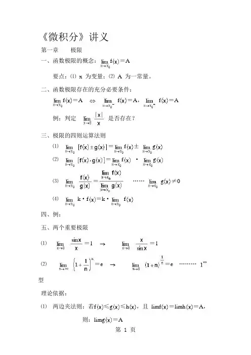
《微积分》讲义第一章极限一、函数极限的概念：f＝A要点：⑴x 为变量；⑵A 为一常量。

二、函数极限存在的充分必要条件：f＝A f＝A，f＝A例：判定是否存在？三、极限的四则运算法则⑴＝f±g⑵＝f·g⑶＝……g≠0⑷k·f＝k·f四、例：五、两个重要极限⑴＝1 ＝1⑵＝e ＝e ………型理论依据：⑴两边夹法则：若f≤g≤h，且limf＝limh＝A，则：limg＝A⑵单调有界数列必有极限。

例题：六、无穷小量及其比较1、无穷小量定义：在某个变化过程中趋向于零的变量。

2、无穷大量定义：在某个变化过程中绝对值无限增大的变量。

3、高阶无穷小，低阶无穷小，同阶无穷小，等价无穷小。

4、定理：f＝A f＝A＋a （a＝0）七、函数的连续性1、定义：函数y＝f在点处连续……在点处给自变量x一改变量x：⑴x0时，y0。

即：y＝0⑵f＝f⑶左连续：f＝f右连续：f＝f2、函数y＝f在区间上连续。

3、连续函数的性质：⑴若函数f和g都有在点处连续，则：f±g、f·g、（g()≠0）在点处连续。

⑵若函数u＝j在点处连续，而函数y＝f在点＝j()处连续，则复合函数f(j(x)) 在点处连续。

例：＝4、函数的间断点：⑴可去间断点：f＝A，但f不存在。

⑵跳跃间断点：f＝A ，f＝B，但A≠B。

⑶无穷间断点：函数在此区间上没有定义。

5、闭区间上连续函数的性质：若函数f在闭区间上连续，则：⑴f在闭区间上必有最大值和最小值。

⑵若f与f异号，则方程f＝0 在内至少有一根。

例：证明方程式－4＋1＝0在区间内至少有一个根。

第二章一元函数微分学一、导数1、函数y＝f在点处导数的定义：x y＝f－f＝A f'＝A ……y'，，。

2、函数y＝f在区间上可导的定义：f'，y'，，。

3、基本初等函数的导数公式：⑴＝0⑵＝n·⑷＝·lnɑ，＝⑸＝cosx，＝－sinx＝x，＝－＝secx·tanx，＝－cscx·cotx4、导数的运算：⑴、四则运算法则：＝·g(x)＋f(x)·例：求下列函数的导数y＝2－5＋3x－7f(x)＝＋4cosx－siny＝⑵、复合函数的求导法则：y u，u v，v w，w x y x例：y＝lntanxy＝lny＝arcsin⑶、隐函数的求导法则：把y看成是x的复合函数，即遇到含有y 的式子，先对y求导，然后y再对x求导。

CHAPTER1Probability Theory1.1.Probability space, (Ω,F,P) (probability space). notations.Definition1.1.(1)Possible outcomesωα,α∈A,are called sample points( )1.(2)The setΩ={ωα:α∈A}=the collection of all possible outcomes,i.e.,the setof all sample points,is called a sample space( ).,Ω .Example1.2.(1)Ω=N=the set of all natural numbers={ωn:ωn= n for all n∈N}.(2)Ω=R=the set of all real numbers.(3)Ω=the collection of all odd positive numbers.(4)Ω=the collection of all fruits,e.g.,apple∈Ω,pineapple∈Ω.(5)Ω=the collection of all colors.Definition1.3.A system F of subsets ofΩis called aσ-algebra if(i)Ω∈F;1A index set. A=N={1,2,3,...}, ωα ωn. A=R, possible outcomes uncountable .56 1.PROBABILITY THEORY(ii)A c∈F whenever A∈F;(iii)A n∈F for all n=1,2,3,...implies that∞n=1A n∈F., ?. , .Example1.4.(1)LetΩ={1,2,3}.Then(i)F1={∅,{1},{2,3},Ω}is aσ-algebra.(ii)F2={∅,{1},{2},{3},Ω}is not aσ-algebra,since{1}∈F2,but{1}c= {2,3}∈F2.(2)LetΩ=R and F=the collection of all subsets of R,then F is aσ-algebra.(3)LetΩ=N.Then(i)F1={∅,{1,3,5,7,...},{2,4,6,8,...},N}is aσ-algebra.(ii)F2={∅,{3,6,9,...},{1,4,7,...},{2,5,8,...},{1,3,4,6,7,9,...},{1,2,4,5,7,8,...}, {2,3,5,6,8,9,...},N}is aσ-algebra.(iii)F3={∅,{1,2},{3,4},{5,6},...,{1,2,3,4},{1,2,5,6},...,{1,2,3,4,5,6},...,Ω} is aσ-algebra.(4)LetΩ=N.Then(i)F1={A⊆N:A isfinite or A c isfinite}is not aσ-algebra.For example,the set A n={n}∈F1for all n,but the set∞n=1A n=N∈F1,since neither N nor N c hasfinite elements.(ii)F2={A⊆N:A is countable or A c is countable}is aσ-algebra., sample space σ-algebra. σ-algebras, Example1.4(3) F1,F2 F3.1.1.PROBABILITY SPACE 7Definition 1.5.Let Ωbe a non-empty set and let F be a σ-algebra on Ω,then (Ω,F )is called a measurable space ( ).Definition 1.6.Let (Ω,F )be a measurable space.A probability measure ( )is a real-valued function P :F −→R satisfying(i)P (E )≥0for all E ∈F ;(ii)(Countable additivity)Let (E n )be a sequence of countable collection of disjointsets in F .ThenP∞ n =1E n =∞ n =1P (E n ).(1.1)(iii)P (Ω)=1.2, σ-algebra A n ∈F for all n =1,2,3,...implies that ∞ n =1A n ∈F . ,(1.1) .Proposition 1.7.(1)P (E )≤1for all E ∈F .(2)P (∅)=0.(3)P (E c )=1−P (E ).(4)P (E ∪F )=P (E )+P (F )−P (E ∩F ).(5)If E ⊆F ,then P (E )≤P (F ).(6)If (E n )is the collection of sets in F ,then P ∞ n =1E n ≤∞ n =1P (E n ).(7)(i)If (E n )satisfiesE 1⊆E 2⊆···⊆E n ⊆···,2 ,P measure.8 1.PROBABILITY THEORY then P (E n )converges to P∞ n =1E n ,i.e.,lim n →∞P (E n )=P ∞ n =1E n .(ii)If (E n )satisfies E 1⊇E 2⊇···⊇E n ⊇···,then P (E n )converges to P∞ n =1E n ,i.e.,lim n →∞P (E n )=P ∞ n =1E n .Definition 1.8.The triple (Ω,F ,P )is called a probability space ( ).Example 1.9.(1)LetΩ={H,T }( ),F ={∅,{H },{T },{H,T }},and let P be given byP (∅)=1,P ({H })=P ({T })=12,P ({H,T })=1.Then (Ω,F ,P )is a probability space.(2)LetΩ={ , , , , , }( ),F =the collection of all subsets of Ω,P satisfies P ({ })=P ({ })=···=P ({ })=1/6and P is a probability measure.Then (Ω,F ,P )is a probability space.(3)Let Ω={ω1,ω2,...,ωn ,...}be a countable set and let F be the collection of allsubsets of Ω.Assume that (p n )be a sequence of real numbers withp n ≥0for all n and ∞n =1p n =1.1.1.PROBABILITY SPACE9 Define a set function P:F−→R by P({ωn})=p n andP(E)=ωn∈E P({ωn})=ωn∈Ep n.Then P defines a probability measure.We call(Ω,F,P)a discrete probability space andΩa discrete sample space.probability space. probability space , notation.Question.Given a sample setΩand a collection of subsets ofΩ,C.Does there exist a collection of subsets ofΩ,say G,such that(i)C⊆G;(ii)G is aσ-algebra?Answer.Yes.We may take G to be the collection of all subsets ofΩ.F C σ-algebra. yes.C⊆H and H:σ-algebraH.σ-algebra : σ-algebra σ-algebra.Notation1.10.If G is the smallestσ-algebra containing C,then we say that G is generated by C and denote it by G=σ(C).Example1.11.LetΩ={1,2,3,4}and C={{1,2},{4}}.Thenσ(C)={∅,{1,2},{3},{4},{1,2,3},{1,2,4},{3,4},Ω}.10 1.PROBABILITY THEORYExample1.12.LetΩ=R and let C be the collection of all open intervals(a,b)in R. Then the sets in B=σ(C)are called Borel sets. , random variable .For example,R,Q,(a,b),[a,b),(a,b],[a,b]are inσ(C). R1 subsets Borel sets. Borel set , real analysis .Remark1.13.LetΩ=[0,1]and let B1be the collection of all Borel sets in[0,1],i.e.,B1=B∩[0,1]:={A∩[0,1]:A∈B}.For(a,b)∈B1,definem((a,b))=b−a.Then we can define a probability measure m:B1−→R.m is called the Lebesgue measure ( ).([0,1],B1,m) probability space .Exercise(1)Find theσ-algebra generated by the given collection of sets C.(a)Ω={1,2,3,4},C={{1,2,3},{4}};(b)Ω={1,2,3,4},C={{2,3,4},{3,4}};(c)Ω={1,2,3,4,5},C={{1,2,4},{1,4,5}};(d)Ω=R,C={[−1,0),(1,2)}(2)LetΩ={1,2,3,4,5,6}and let F=σ({{1,2,3,4},{3,4,5}}).Find a probabilitymeasure defined on(Ω,F).1.2.RANDOM VARIABLES11 (3)Consider a probability space(Ω.F,P),whereΩ={1,2,3,4,5},F is the collectionof all subsets ofΩ,andP({1})=P({2})=P({5})=14,P({3})=P({4})=P({6})=112.(a)LetX=2I{1}+3I{2,3}−3I{4,5}+I{6}.Find E[X]and E[X2].(b)LetY=I{1,2}+3I{2,4,5}−2I{4,5,6}.Find E[Y]and E[Y3].(4)LetΩ=R,F=all subsets so that A or A c is countable,P(A)=0in thefirstcase and=1in the second.Show that(Ω,F,P)is a probability space,i.e.,show that F is aσ-algebra and P is a probability measure.1.2.Random variablesLet(Ω,F,P)be a probability space.Definition1.14.We say a function X:Ω−→R to be a random variable(r.v., )if for every B∈B,{ω:X(ω)∈B}∈F,i.e.,X is measurable with respect to F.Notation1.15.For all random variable X and B∈F,{X∈B}:={ω∈Ω:X(ω)∈B}.12 1.PROBABILITY THEORYExample1.16.Suppose thatΩ=[0,1]and F=B1.(1)X1(ω)=ω.For B∈B,{X1∈B}={ω∈[0,1]:X1(ω)∈B}={ω∈[0,1]:ω∈B}=B∩[0,1]∈B1.Thus,X1is a random variable.(2)X2(ω)=ω2.For B∈B,{X2∈B}={ω∈Ω:X2(ω)∈B}={ω∈Ω:ω2∈B}., B∈B .. Example1.18(1) .Theorem1.17.The following statements are equivalent.(1)X is a random variable on(Ω,F).(2){X≤r}∈F for all r∈R.(3){X<r}∈F for all r∈R.(4){X≥r}∈F for all r∈R.(5){X>r}∈F for all r∈R., check random variable . Example1.16 X2 , check X2(ω)=ω2 random variable B , , . Theorem1.17 .Example1.18.(1)ConsiderΩ=[0,1],F=B1and X(ω)=ω2.(i)If r<0,{X≤r}={ω∈[0,1]:ω2≤r}=∅∈F.1.2.RANDOM VARIABLES13(ii)If0≤r≤1,{X≤r}={ω∈[0,1]:ω2≤r}=[0,√r]∈F.(iii)If r>1,{X≤r}=[0,1]∈F.Thus,X is a random variable.(2) random variable .LetΩ={1,2,3,4}and F=σ({1,2},{3},{4}).(a)X1(1)=2,X1(2)=3,X1(3)=4,X1(4)=5.Since{X1≤2}={1}∈F,X1is not a random variable.(b)X2(1)=X2(2)=2,X2(3)=10,X2(4)=−500.(i)If r<−500,{X2≤r}=∅∈F.(ii)If−500≤r<2,{X2≤r}={4}∈F.(iii)If2≤r<10,{X2≤r}={1,2,4}∈F.(iv)If r≥10,{X2≤r}=Ω∈F.Thus,X2is a random variable.Theorem1.19.(1)If X is a random variable,f is a Borel measurable function on(R,B),then f(X)is a random variable.(2)If X and Y are random variables,f is a Borel measurable function of two vari-ables,then f(X,Y)is a random variable.(3)If(X n)n≥1is a sequence of random variables,theninf n X n,supnX n,lim infn→∞X n,lim supn→∞X n,limn→∞X nare random variables., .lim sup lim inf Appendix A .14 1.PROBABILITY THEORYExample1.20.(1)Let(Ω,F,P)be a discrete probability space.Then every real-valued function onΩis a random variable.(2)Let(Ω,F,P)=([0,1],B1,m).Then the random variables are exactly the Borelmeasurable functions defined on([0,1],B1).Exercise(1)LetΩ={1,2,3,4,5,6},and letX1(ω)=⎧⎪⎪⎪⎪⎪⎪⎪⎪⎪⎪⎪⎪⎪⎪⎪⎨⎪⎪⎪⎪⎪⎪⎪⎪⎪⎪⎪⎪⎪⎪⎪⎩1,ω=1,2,ω=2,1,ω=3,1,ω=4,2,ω=5,2,ω=6,X2(ω)=⎧⎪⎪⎪⎪⎪⎪⎪⎪⎪⎪⎪⎪⎪⎪⎪⎨⎪⎪⎪⎪⎪⎪⎪⎪⎪⎪⎪⎪⎪⎪⎪⎩3,ω=1,2,ω=2,3,ω=3,3,ω=4,2,ω=5,2,ω=6,X3(ω)=⎧⎪⎪⎪⎪⎪⎪⎪⎪⎪⎪⎪⎪⎪⎪⎪⎨⎪⎪⎪⎪⎪⎪⎪⎪⎪⎪⎪⎪⎪⎪⎪⎩3,ω=1,2,ω=2,1,ω=3,5,ω=4,4,ω=5,4,ω=6.(a)Let F=σ({{1},{2},{3},{4},{5},{6}}),which of X1,X2,X1+X2,X1+X3and X3are random variables on(Ω,F)?(b)Let F=σ({{1,2,3},{4,5}}),which of X1,X2,X1+X2,X1+X3and X3are random variables on(Ω,F)?(c)Let F=σ({{1,4},{2,5},{3}}),which of X1,X2,X1+X2,X1+X3andX3are random variables on(Ω,F)?(2)Suppose X and Y are random variables on(Ω,F,P)and let A∈F.Show thatif we letZ(ω)=⎧⎪⎨⎪⎩X(ω),ifω∈A,Y(ω),ifω∈A c,then Z is a random variable.(3)Let P be the Lebesgue measure onΩ=[0,1].DefineZ(ω)=⎧⎪⎨⎪⎩0,if0≤ω<1/2,2,if1/2≤ω≤1.For A∈B1,defineQ(A)=AZ(ω)d P(ω).(a)Show that Q is a probability measure.(b)Show that if P(A)=0,then Q(A)=0.(We say that Q is absolutelycontinuous with respect to P.)(c)Show that there is a set A for which Q(A)=0but P(A)>0.1.3.ExpectationDefinition1.21.The functionI A(ω)=⎧⎪⎨⎪⎩0,ifω∈A,1,ifω∈A.is called the indicator function of A.Remark1.22.The indicator function I A is a random variable if and only if A∈F.Definition1.23.(1)Let A i∈F for all i and let a random variable X be of the formX=∞i=1b i I A i.(1.2)Then X is called a simple random variable.(2)Let X be the form(1.2),we define the expectation( )of X to beE[X]=∞i=1b i P(A i)., .(A n) disjoint.Example1.24.Let(Ω,F,P)=([0,1],B1,m)and considerX=∞i=112iI[0,2−i).Then the expectation of X is given byE[X]=∞i=112iP([0,2−i))=∞i=114i=13.Remark1.25.Consider the generalization of the expectation3.Let X be a positive random variable.DefineΛmn=ω:n2m≤X(ω)<n+12m∈F,for all m,n∈N.LetX m=∞n=0n2mIΛmn.(X m Figure1.3)Due to the construction of X m,we see that for allω∈Ω, X m(ω)↑andlimm→∞X m(ω)=X(ω).(i)If E[X m]=+∞for some m,we define E[X]=+∞.3 Lebesgue integral, . Riemann integral .Riemann inegral ,Lebesgue integral . . step functions/simple functions, simple functions f . Figure1.1 Figure1.2.Figure1.1.Riemann integralFigure1.2.Lebesgue integral (ii)If E[X m]<∞for all m,defineE[X]=limm→∞E[X m]=limm→∞∞n=0n2mPn2m≤X<n+12m.positive random variable expectation,Definition1.26.Consider a general random variable X.Then we can write X asX=X+−X−,where X+=X∨0,X−=(−X)∨0.3.2.4.Figure1.3.X X m(1)Unless both of E[X+]and E[X−]are+∞,we defineE[X]=E[X+]−E[X−].(2)If E|X|=E[X+]+E[X−]<∞,X has afinite expectation.We denote byE[X]=ΩX d P=ΩX(ω)P(dω).(3)For A∈F,defineAX d P=E[X I A],(1.3) which is called the integral of X with respect to P over A.(4)X is integrable with respect to P over A if the integral(1.3)exists and isfinite. Remark1.27.(1)If X has a cumulative distribution function(c.d.f.)F withrespect to P,thenE[X]= ∞−∞x dF(x).Moreover,if g is Borel measurable function in R,E[g(X)]= ∞−∞g(x)dF(x).(2)If X has a probability density function(p.d.f.)f with respect to P,thenE[X]= ∞−∞xf(x)dxandE[g(X)]= ∞−∞g(x)f(x)dx.(3)If X has a probability mass function p with respect to P,thenE[X]=∞n=1x n p(x n),E[g(X)]=∞n=1g(x n)p(x n).Example1.28.(1)LetΩ={1,2,3,4},F=σ({1},{2},{3},{4})andP({1})=12,P({2})=14,P({3})=16,P({4})=112.LetX=5I{1}+2I{2}−4I{3,4}. ThenE[X]=5·12+2·12−416+112=2E[X2]=25·12+4·12+1616+112=352.(2)Suppose X is normally distributed on(Ω,F,P)with mean0and variance1,thenX has probability density function1√2πexp−x22.Thus,E[X]= ∞−∞x1√2πexp−x22=0,E[X3]= ∞−∞x31√2πexp−x22=0,(odd function)E[e X]= ∞−∞e x1√2πexp−x22=1√2π∞−∞exp−x22+xdx=1√2π∞−∞exp−12(x−1)2+12dx=e1/2.Proposition1.29.(1)(Absolute Integrability)A X d P<∞⇐⇒A|X|d P<∞.4(2)(Linearity)A (aX+bY)d P=aAX d P+bAY d P.(3)(Additivity over sets)If(A n)is disjoint,then∪n A n X d P=nA nX d P.(4)(Positivity)If X≥0P-a.e.5on A,thenAX d P≥0.(5)(Monotonicity)If X1≤X≤X2P-a.e.on A,thenA X1d P≤AX d P≤AX2d P.4 Riemann integral .5We say a property holds P-a.e.(almost everywhere)or P-a.s.(almost surely)means that the probability that this property holds is equal to1,i.e.,except a set with probability0,this property is true.(6)(Modulus Inequality)AX d P≤ A|X |d P .Theorem 1.30.(1)(Dominated Convergence Theorem)If lim n →∞X n =X P -a.e.on A and |X n |≤Y P -a.e.on A for all n withAY d P <∞.Thenlim n →∞AX n d P =A lim n →∞X n d P =AX d P .(2)(Monotone Convergence Theorem)If X n ≥0and X n X P -a.e.on A ,thenlimn →∞AX n d P =A lim n →∞X n d P =AX d P .(3)(Fatou’s Lemma)If X n ≥0P -a.e.on A ,thenA lim inf n →∞X n d P ≤lim infn →∞AX n d P .(4)(Jensen’s Inequality)If ϕis a convex function,X and ϕ(X )are integrable,thenϕ(E [X ])≤E [ϕ(X )].Exercise(1)Let λbe a fixed number in R ,and define the convex function ϕ(x )=e λx forall x ∈R .Let X be a normally distributed random variable with mean μand variance σ2,i.e.,the probability density function of X is given byf (x )=1√2πσexp −(x −μ)22σ2 .(a)Find E [e λX ].(b)Verify that Jensen’s inequality holds (as it must):E ϕ(X )≥ϕ(E [X ]).(2)For each positive integer n ,define f n to be the normal density with mean zeroand variance n ,i.e.,f n (x )=1√2nπexp −x22n.(a)What is the function f (x )=lim n →∞f n (x )?(b)What is limn →∞∞−∞f n (x )dx ?(c)Note thatlimn →∞∞−∞f n (x )dx =∞−∞f (x )dx.Explain why this does not violate the ”Monotone Convergence Theorem”.(3)Let P be the Lebesgue measure on Ω=[0,1].Define Z (ω)=⎧⎪⎨⎪⎩0,if 0≤ω<1/2,2,if 1/2≤ω≤1.For A ∈B 1,defineQ (A )=AZ (ω)d P (ω).(a)Show that Q is a probability measure.(b)Show that if P (A )=0,then Q (A )=0.(We say that Q is absolutelycontinuous with respect to P .)(c)Show that there is a set A for which Q (A )=0but P (A )>0.。

微积分入门通俗讲义汇编序中国战国时代（公元前7世纪），我国的庄周所著的《庄子》一书的“天下篇”中，记有“一尺之棰，日取其半，万世不竭”，即老庄哲学中所有的无限可分性和极限思想；公元前4世纪《墨经》中有了有穷、无穷、无限小（最小无内）、无穷大（最大无外）的定义和极限、瞬时等概念。

这是朴素的、也是很典型的极限概念。

而极限理论便是微分学的基础。

古希腊时期（公元前3世纪），阿基米德用内接正多边形的周长来穷尽圆周长，而求得圆周率愈来愈好的近似值，也用一连串的三角形来填充抛物线的图形，以求得其面积。

这是穷尽法的古典例子之一，可以说是积分思想的起源。

17世纪，许多著名的数学家、天文学家、物理学家都为解决上述几类问题作了大量的研究工作，如法国的费马、笛卡尔、罗伯瓦、笛沙格；英国的巴罗、瓦里士；德国的开普勒；意大利的卡瓦列利等人都提出许多很有建树的理论。

为微积分的创立做出了贡献。

17世纪下半叶，在前人工作的基础上，英国大科学家牛顿和德国数学家莱布尼茨分别在自己的国度里独自研究和完成了微积分的创立工作，虽然这只是十分初步的工作。

19世纪初，法国科学学院的科学家以柯西为首，对微积分的理论进行了认真研究，建立了极限理论，后来又经过德国数学家维尔斯特拉斯进一步的严格化，使极限理论成为了微积分的坚定基础。

才使微积分进一步的发展开来。

1874年，德国数学家外尔斯特拉斯构造了一个没有导数的连续函数，即构造了一条没有切线的连续曲线，这与直观概念是矛盾的。

它使人们认识到极限概念、连续性、可微性和收敛性对实数系的依赖比人们想象的要深奥得多。

外尔斯特拉斯最终完成了对实数系更深刻的性质的理解，使得数学分析完全由实数系导出，脱离了知觉理解和几何直观。

人类对自然的认识永远不会止步，微积分这门学科在现代也一直在发展着，人类认识微积分的水平在不断深化。

微积分学(Calculus, 拉丁语意为用来计数的小石头) 是研究极限、微分学、积分学和无穷级数的一个数学分支，并成为了现代大学教育的重要组成部分。

Chapter 1 The real number system1.3. Completeness axiom of R1.16 DefinitionLet R E ⊆ and φ≠E .(i).The set E is said to be bounded above if there is an R M ∈ s.t M a ≤ for allE a ∈.(ii).A number M is called an upper bound of the set E if M a ≤ for all E a ∈. (iii).A number S is called a supremum of the set E if S satisfies the followingconditions(1) if E a S a ∈∀≤,,(2) if M is an upper bound of E then M S ≤.Remark The supremum is also called the least upper bound.1.17: ExampleIf E=[0,1], prove that 1 is a supremum of E .Proof.1. ]1,0[,1=∈∀≤E a a .2. let M be an upper boundthen M a ≤ for all ]1,0[∈a])1,0[1(1∈≤⇒ M .We derive the result.1.18: RemarkIf a set has one upper bound, it has infinitely many upper boundsProof:. Let E be a subset of R .Let M a ≤ for all E a ∈.Then M is an upper bound.Let R b b ∈>,0 then M+b is also an upper bound.So, E has infinitely many upper bounds.1.19 . Theorem. Let E be a nonempty subset of R . Then the least upper bound of E is unique if it exists.Proof.Suppose that 21&s s are the least upper bounds of E.Then 21&s s are upper bounds of E .1221&s s s s ≤≤∴21s s =∴.NotationThe supremum is also called least upper bound . We use sup E to denote the supremum of nonempty set E .1.20. Theorem [Approximation property]E E R E sup and ,,φ≠⊆exists. Then E a ∈>∀an is there ,0ε s.t E a E sup sup ≤<-ε.Proof:. Suppose the conclusion is false. There is an 0>ε such that.,sup E a E a ∈∀-≤ε.ε-∴E sup is an upper bound.→←≥-⇒E E sup sup ε0>εE a ∈∃∴ s.t E a E sup sup ≤<-ε1.21. TheoremIf N E ⊆ has a supremum, then E E ∈supProof.Let supE=s.By Approximation property, there E x ∈∃0 s.t s x s ≤<-01.If s x =0 then E E ∈sup is obvious.If s x s <<-01, thenE x ∈∃1 s.t 001100x s x x s x x -≤-<⇒≤<.1. 1,0101≥-⇒∈x x N x x .2. 1)1(1,0101=--<-⇒->≥s s x x s x x s .It is a contradiction.E E ∈∴sup● [Complete axiom of R ]Every nonempty subset E of R that is bounded above,then E has the least upper bound. .1.22 :[Archimedean Principle]N n b a R b a ∈∃⇒>∈0,,, s.t b<na.Proof:1. If b<a , then take n=1.2. If a<b , let };{b ka N k E ≤∈=.φ≠∴∈E E ,1 .⇒∈∀≤E k ab k ,E is bounded above. By Completeness of R , sup E exists.ba E E E E E >+∴∉+∴∈⇒)1(sup 1sup )21.1 Theorem by (suptake n=supE+11.23: Example.Let ,.......}41,21,1{=A and ,...}87,43,21{=B prove that supA=supB=1Proof.1. 1{;0}2n A n N or n =∈= 11,,0,1,2,..2n x x n ≥==. 1∴ is an upper bound.Let M be another bound..1sup 1210=∴=≥∴A M 2. };211{N n B n ∈-= N n n∈∀-≥,2111 1∴ is an upper bound of B.Let M be an upper bound of BTo show 1≥M .Suppose not 011>-⇒<⇒M MBy Archimedean principle, there exists N n ∈ such that M n-<11, M n-<∃⇒121 for some N n ∈. →←>-⇒-->-=-∴M M n n n n n 212)1(1212211 M is an upper bound. 1≥∴M1sup =∴B● [Well-Order Principle]⇒≠⊆φE N E ,E has a least element(ie.E a ∈∃ s.t E x x a ∈∀≤,)1.24. Theorem (Density of rational)Let R b a ∈, satisfy a<b , then there is a rationalnumber c s.t a<c<b.Proof:Let N n a b n∈-<,1(by Archimedean Principle). 1. If b>0, let }.;{nk b N k E ≤∈= By Archimedean Principle φ≠⇒E .By Well-Order Principle ⇒E has a least element, says 0k . .)..(1:0b n m e i E m k m <∉⇒-=∴ Let nm q =. We must show that a<q<b.q<b is obvious, now we show that a<q....11)(00b q a a q q n k n n k a b b a <<∴>∴=-=-<--=2. If b<0, then0>∃k , k is a natural number s.t b+k>0.Q c ∈∃∴ s.t a+k<c<b+kQk c Q c bk c a ∈-⇒∈<-<∴ie. There is a rational number between a & b.1.27. Definition.φ≠⊆E R E ,.1. s is called a lower bound of E if E x s x ∈∀≥,.In the case, E is called bounded below2.t is called the greatest lower bound of Eif1.Extx∈∀≥,,2. If M is a lower bound of E then tM≤.3.E is bounded if ExMx∈∀≤,for some M>0. (i.e. E is bounded above and below.)●Let E be a set of R. We define };{ExxE∈-=-.1.28. Theoremφ≠⊆ERE,.1.sup E exists ⇔inf(-E) existsin fact supE= -inf(-E)2.inf E exists⇔sup(-E) existsin fact inf E= -sup(-E)Proof:1.""⇒supE exists.Now we show that –supE=inf(-E).Show that 1.-sup E is a lower bound of –E.2. if s is a lower bound of EsE sup-≤⇒-.1.Esupis an upper bound of EExExExEx∈∀-≥-⇒∈∀≤∴,sup,supEsup-∴is a lower bound of –E2. Suppose that s is a lower bound of -ESuppose not EsEs supsup<-⇒->⇒on the other hands xE xs x-≤∴∈∀≥-,Hence, -s is a upper bound of E→←By 1.& 2, EEE sup)inf(&)inf(-=-∃-.The proof of converse is similar.Remark. The largest lower bound is also called infimum. Remark. The completeness axiom of R is equivalent to“ Every nonempty, bounded below subset of R has the infimum”.1.29. Theorem.inf inf ,sup sup ,,A B A B B A R B A ≤≥⇒≠⊆⊆φif B B inf and sup exist.Hence, B A A B sup sup inf inf ≤≤≤Proof:1. suppose sup B exists.,sup .,sup A x B x B A B x B x ∈∀≤∴⊆∈∀≤∴A ∴ is bounded above & supB is an upper bound of ABy complete axiom of R, .sup sup &sup B A A ≤∃2. S ppose that inf B exists..,inf ,inf A x B x B A Bx B x ∈∀≥∴⊆∈∀≥∴A ∴ is bounded below & infB is an lower bound of A.By complete axiom of R, B A A inf inf &:inf ≥∃.Def:sup ,inf φφ=-∞=∞1.4 Functions, countability and the algebra of sets.DefinitionLet A & B be two sets of R.A function f is a relation between A &B s.t f assigns each element x of A to aunique By∈Definition:f→ABf is called 1-1 if )x≠y⇒≠f(yx)(fDef::f→BAf is called onto if A∈∀,s.t f(x)=y∃xBy∈Definition 1.34:Let E be s a set of R.1. E is said be finite if φ&∃}...3,2,1{∈.....},2,1{:=n→E or EnnNfs.t f is 1-1 & onto.2. E is called countably infinite if E∃:s.t f is 1-1 & onto.Nf→3. E is called countable if E is finite or countably infinite.4. E is called uncountable if E is not countable1.35. Theorem .The open interval (0,1) is uncountablePf:Suppose (0,1) is countable.Then there is a list for (0,1) says.....................................................................0............................................................................0.........0.........0321333231323222121312111n n n n a a a a a a a a a a a a a a a a ==== Let .......0321ααα=x where {=k α10==k k αα .1f ,1if ≠=kk kk a i a kk k a ≠∴α x ∴ is not in this list →← (0,1) is uncountable1.37. TheoremB B A ,⊆ is countable A ⇒ is countable1.38 Theoremn A A A ,......,21 are countable. },:{:1N j A x x A A E j j j N j j∈∈===∞=∈ .If j A is countable for E N j ⇒∈ is countable.。