maple绘图

第6章 Maple 中作图6.1 二维函数作图命令plot6.1.1 二维函数作图用plot 命令可以画出一元函数在指定区间上的二维函数图形。

其用法有plot （函数，变量名） plot （函数，范围，选项)范围和选项均可省略，缺省时系统自动选取最佳设置。

最简单的plot 语句为plot(f(x),x=a..b) 画出f(x)在区间[a,b]上的图像，其中f 可为过程或表达式。

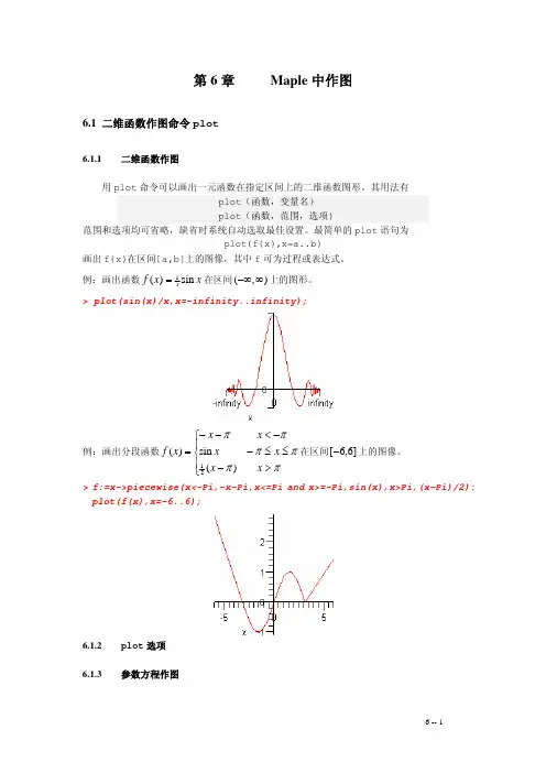
例：画出函数x x f sin )(1=在区间),(∞−∞上的图形。

> plot(sin(x)/x,x=-infinity..infinity);例：画出分段函数⎪⎩⎪⎨⎧>−≤≤−−<−−=ππππππx x x x x x x f )(sin )(21在区间]6,6[−上的图像。

> f:=x->piecewise(x<-Pi,-x-Pi,x<=Pi and x>=-Pi,sin(x),x>Pi,(x-Pi)/2):plot(f(x),x=-6..6);6.1.2 plot 选项 6.1.3 参数方程作图用plot 函数画参数曲线的一般形式为plot （[x(t),y(t),t=a..b]，选项） 或plot （[[x(t),y(t),t=a..b],[u(t),v(t),t=c..d]]，选项）在一个坐标系中同时画两条参数曲线。

例 ：画参数曲线]2,0[sin cos 1π∈⎩⎨⎧=+=t t y tx ，。

> plot([1+cos(t),sin(t),t=0..2*Pi]);6.1.4 特殊坐标系下作图plot 通常画的是直角坐标下的函数图像，通过设置coords 选项，plot 也可以画出特殊坐标下的函数图像。

例如，画出极坐标下函数b t a t r r ≤≤=，)(的图形可用命令plot(r(t),t=a..b,coords=polar) 或 plot([r(t),t,t=a..b],coords=polar)在6.3小节中，还将给出plots 程序包中画特殊坐标系下的函数图像的命令，例如polarplot(r(t),t=a..b)例 ：特殊坐标系下的函数图像。

(第六章M aple的绘图功能)§6.3 三维图形绘制三绘图原理上，三维图形与二维图形没有本质的区别，但由于涉及到如何在二维的显示设备上表示的问题，在图形学中，三维图形增加了投影方式的选择。

然而在Maple系统中，用户却不需要考虑投影方面的问题，因为几乎所有的三维图形都是以斜投影的方式表示的。

用户可以改变的，只有物体的方向以及视点的远近。

由于三维图形绘制时可以选择的参数同二维图形基本类似，所以在对plot3d函数做基本介绍后，本节的重点将转移到一些plot程序库附带的其他三维图形绘制函数上，比如等高线、密度图等的绘制。

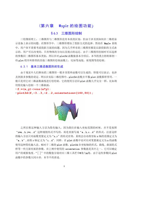
6.3.1 基本三维函数图形的生成由于现实中人们熟知的三维图形一般并非简单函数可以生成的，即使可以表示，也涉及到很多参数的设定，所以在实际三维绘图中，plot3d函数并不像plot函数那样常用。

一般只是用它对三维函数曲线进行绘绘制。

它的使用方法同plot函数几乎完全一样，比如利用简化输入绘制一个三维曲面：> f:=(x,y)->cos(x*y):> plot3d(f,-3..3,-2..2,orientation=[160,50]);之所以称这种输入方法为简化输入，因为我们在输入坐标范围的时候，并不是按照“x=a..b,y=c..d”这种规则形式书写的，而是直接写成“a..b,c..d”的形式。

注意这样的输入方法只对函数变量定义为“x,y”的形式有效，系统会自动将坐标x轴的范围定义为“a..b”,而将y轴定义为“c..d”。

同样，在plot函数中也可以对变量被定义为x的函数使用这种简化输入法。

相对于二维的plot函数，plot3d在坐标轴的形式，曲线、曲面的式样等一些方面有新的参数。

在上例中使用的orientation参数就是其中之一，它可以确定用户的观察角度。

“[ ]”中的数值分别对应三维工具栏中θ角与ϕ角。

由于这些参数同plot 函数中的参数大同小异，本节不再讲述。

Maple在数学作图中的应用数学图像在数学中是非常重要的，通过数学图像我们可以解决很多难以计算或证明的问题，同时，图像往往能给人一种比较直观易懂的感觉，因而有时利用作图的方法解决数学问题时会起到柳暗花明的奇效。

但是，不是所有的图像都是那么容易作出来的。

在很多情况下，我们虽然能给出其表达式，却难以或者无法真正作出来，甚至有时连直观想象都很困难。

这时，运用Maple作图就显得非常方便了。

Maple具有强大的作图功能，它的作图方法也非常简单方便，只需输入简短的指令操作即可，当然函数表达式必须给出的，不论用参数方程，还是在不同的坐标系下作图，Maple都可以很好地完成任务，以下我以Maple 13为例，主要从多个例子来说明Maple在数学作图中的应用。

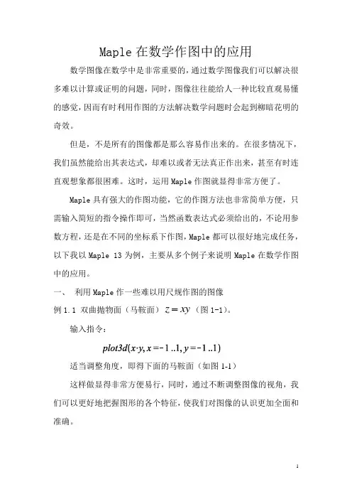
一、利用Maple作一些难以用尺规作图的图像（图1-1）。

例1.1 双曲抛物面（马鞍面）z xy输入指令：适当调整角度，即得下面的马鞍面（如图1-1）这样做显得非常方便易行，同时，通过不断调整图像的视角，我们可以更好地把握图形的各个特征，使我们对图像的认识更加全面和准确。

图1-1例1.2 函数441(,),,1sin cos f x y x y x x ππ=-≤≤++的图像。

输入指令：适当调整角度即得 图1-2例1.3 球面z=z=所围成立体及其表面。

输入指令：适当调整角度即得图1-3像例1.3中的这种类型的图像（曲面或者所围成的立体图形）在多元函数的积分中非常常见，通常作为多元函数积分的积分区域，通常这种区域是很难用尺规作图的，很大方面都要凭我们的空间想象。

而利用Maple作图，可以很好的展现图形的各个角度的情况，使图形显得十分直观(当然我们也可以直接用Maple计算积分)。

例1.4 阿基米德螺旋面()()(),02,,05,2u x y s t v x y s s s w x y ππ⎧=⎪⎪≤≤⎪=-⎨≤≤⎪⎪=+⎪⎩输入指令： plot3d适当调整角度，即得图1-4例1.5 在柱坐标和球坐标下函数(),cos f r r θθ=的图形。

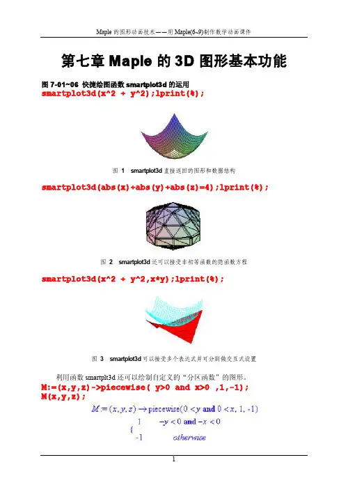
第七章Maple的3D图形基本功能图7-01~06快捷绘图函数smartplot3d的运用smartplot3d(x^2+y^2);lprint(%);图1smartplot3d直接返回的图形和数据结构smartplot3d(abs(x)+abs(y)+abs(z)=4);lprint(%);图2smartplot3d还可以接受非初等函数的隐函数方程smartplot3d(x^2+y^2,x*y);lprint(%);图3smartplot3d可以接受多个表达式并可分别做交互式设置利用函数smartplt3d还可以绘制自定义的“分区函数”的图形。

M:=(x,y,z)->piecewise(y>0and x>0,1,-1);M(x,y,z);smartplot3d(M(x,y,z));lprint(%);图4利用smartplot3d绘制“分区函数”的图形（做过交互式设置）smartplot3d函数具有multyple功能，因而可以绘制曲面族的图形。

smartplot3d(seq(x^2+y^2+125*i,i=1..4));图5利用smartplot3d函数的multyple功能绘制曲面族的图形可以把smartplot3d函数返回的图形数据结构拷入一个执行组，并添加一些plot设置选项，再次执行。

INTERFACE_SMARTPLOT3D([x^2+y^2,x,y,_NoZ],style=LINE,a xes=frame,color=blue);lprint(%);图6把图１的返回数据拷入一个执行组，并添加一些设置选项，再次执行的结果图73D图形窗口图83D图形工具栏的第一组图93D图形工具栏的第二组图10各钮对应的图形样式图113D图形工具栏的第三组图12不同样式的坐标架图13Style级联菜单图14Color级联菜单INTERFACE_SMARTPLOT3D([x^2+y^2-z^2=1,x,y,z],color=cya n,view=[-3..3,-3..3,-2..2]);图15按着命令语句生成的图形图16鼠标指向图形，颜色变得灰暗图17选中color命令引出级联菜单图186条命令的不同着色效果图19使用曲面样式选项和颜色选项分别设置的实例图20坐标架的四种样式图21Ranges命令可确定各个坐标轴的显示范围图22Projection级联菜单图23不同的投影类型图24绘制3D图形的子菜单命令图25从返回信息中选定一个三元表达式，绘制快捷图形图26从返回信息中选定一个二元表达式，绘制3D快捷图形图27从返回信息中选定一个二元表达式，绘制2D快捷图形图28从返回信息中选定一个一元表达式，绘制2D快捷图形图29从返回信息中选定一个一元表达式，绘制3D快捷图形图30 6.0中选定单变量表达式只能绘制2D图形图317.0中选定单变量表达式还能绘制3D图形图7-32~34plot3d的调用语句plot3d(x*exp(-x^2-y^2),x=-2..2,y=-2..2,color=green);图32用plot3d绘制单片曲面plot3d([sin(x)*cos(y),sin(x)*sin(y),cos(x)],x=0..Pi/2, y=0..x);图33用plot3d绘制参数曲面plot3d([x,y,sqrt(4-x^2-y^2)],x=-1.999..1.999,y=-sqrt( 4-x^2)+1/920..sqrt(4-x^2),grid=[15,35]);图34参数曲面，变量y的范围界线是x的函数图7-35~41plot3d的调用语句的设置选项plot3d(1,t=0..2*Pi,p=0..Pi,orientation=[50,70],scalin g=constrained,axes=box);plot3d(1,t=0..2*Pi,p=0..Pi,coords=cylindrical,scaling =constrained,orientation=[50,70],axes=box);plot3d(1,t=0..2*Pi,p=0..Pi,coords=spherical,scaling=c onstrained,orientation=[50,70],axes=box);图35表达式“1”在三种坐标系（直角系、圆柱系、球面系）中的图形plot3d(v,u=0..2*Pi,v=-1..1,title=`CONE`,scaling=uncon strained,orientation=[50,70],axes=box);plot3d(v,u=0..2*Pi,v=-1..1,coords=cylindrical,title=` CONE`,scaling=unconstrained,orientation=[50,70],axes= box);plot3d(v,u=0..2*Pi,v=-1..1,coords=spherical,title=`CONE`,scaling=unconstrained,orientation=[50,70],axes=bo x);图36表达式“v ”在三种坐标系（直角系、圆柱系、球面系）中的图形plot3d(u,u=0..2*Pi,v=-2..2,title=`CONE`,scaling=uncon strained,orientation=[50,70],axes=box);plot3d(u,u=0..2*Pi,v=-2..2,coords=cylindrical,title=`CONE`,scaling=unconstrained,orientation=[50,70],axes=box);plot3d(u,u=0..2*Pi,v=-2..2,coords=spherical,title=`CO NE`,scaling=unconstrained,orientation=[50,70],axes=bo x);图37表达式“u ”在三种坐标系（直角系、圆柱系、球面系）中的图形plot3d((1.3)^x*sin(y),x=-1..2*Pi,y=0..Pi,style=patch);plot3d((1.3)^x*sin(y),x=-1..2*Pi,y=0..Pi,coords=cylin drical,style=patch);plot3d((1.3)^x*sin(y),x=-1..2*Pi,y=0..Pi,coords=spher ical,style=patch);图38表达式“(1.3)^x*sin(y)”在三种坐标系（直角系、圆柱系、球面系）中的图形范围的端值可以使用变量在某些情况下，范围的端值可以使用变量。

第五章绘图：作图有两个软件包。

(1)图形软件包，用with(plots)调入。

(2)图形工具包with(plottools)图形包)中有下列作图命令：animate, animate3d动画changecoords改变坐标系complexplot, complexplot3d复函数图conformal contourplot contourplot3d coordplot coordplot3d cylinderplot柱坐标函数图densityplot密度图display display3d图函数显示fieldplot fieldplot3d区域图gradplot gradplot3d梯度图implicitplot implicitplot3d 隐函数图inequal listcontplot listcontplot3d listdensityplot listplot listplot3d loglogplot logplot matrixplot odeplot微分方程数值解图pareto pointplot pointplot3d点图polarplot极坐标图polygonplot polygonplot3d多边形图polyhedraplot replot rootlocus semilogplot setoptions setoptions3d作图选项设置spacecurve空间曲线图sparsematrixplot sphereplot球坐标图surfdata textplot textplot3d tubeplot工具包中有下列图形工具：arc弧arrow 箭头circle圆cone 圆锥cuboid长方体curve曲线cutin cutout cylinder柱disk 圆盘dodecahedron十二面ellipse椭圆ellipticArc椭圆弧hemisphere半球hexahedron 六面体hyperbola双曲线icosahedron二十面体line线段octahedron八面体pieslice point点polygon多边形rectangle矩形semitorus sphere球tetrahedron四面体torus轮第一节二维曲线图：一．基本命令(不需调图形包)plot({f1(x)，f2(x),…},x=a..b，选项)；一元函数曲线plot(f,a..b，选项); 作过程函数图x=a..b(中间两点)表示变量x在[a,b]区间。

Maple作图命令详解在使用Maple进行计算的时候，很多情况下需要对函数进行绘图以便能够进行更深入的研究与说明，那么，在Maple中怎样作图呢？作图的命令有哪些呢？作图有两个软件包。

（1）图形软件包，用with(plots)调入。

（2）图形工具包with(plottools)图形包中有下列作图命令：animate、animate3d 动画；changecoords 改变坐标系；complexplot、complexplot3d复函数图；conformal、contourplot、contourplot3d、coordplot、coordplot3d、cylinderplo柱坐标函数图；densityplot密度图；display、display3d图函数显示；fieldplot、fieldplot3d区域图；gradplot、gradplot3d梯度图；implicitplot、implicitplot3d隐函数图；inequal listcontplot、listcontplot3d listdensityplot、listplot listplot3d、loglogplot、logplot、matrixplot、odeplot微分方程数值解图；pareto pointplot、pointplot3d点图；polarplot极坐标图；polygonplot、polygonplot3d多边形图；polyhedraplot、replot、rootlocus semilogplot、setoptions setoptions3d作图选项设置；spacecurve空间曲线图；sparsematrixplot、sphereplot球坐标图；surfdata textplot、textplot3d、tubeplot工具包中有下列图形工具：arc弧，arrow箭头，circle圆，cone圆锥，cuboid长方体，curve曲线，cutin cutout cylinder 柱，disk圆盘，dodecahedron十二面，ellipse椭圆，ellipticArc椭圆弧，hemisphere半球，hexahedron 六面体，hyperbola双曲线，icosahedron，二十面体，line线段，octahedron八面体，pieslice point点，polygon 多边形，rectangle矩形，semitorus、sphere球，tetrahedron四面体，torus轮Maple绘图示例基本命令（不需调图形包）一元函数曲线作过程函数图x=a..b(中间两点)表示变量x在[a,b]区间。

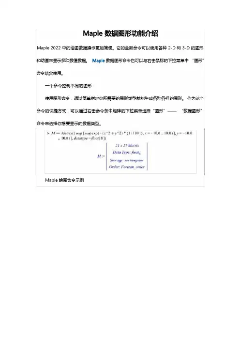
Maple 2022 中的绘图数据操作更加简便。

它的全新命令可以使用各种 2-D 和 3-D 的图形和动画来显示多种数值数据。

数据图形命令也可以与右击鼠标的下拉菜单中“图形”命令结合使用。

一个命令控制不同的图形：使用图形命令，通过简单指定你所需要的图形类型就能生成各种各样的图形。

作为这个命令的快捷方式，可以通过右击命令条中矩阵的下拉菜单选择“图形”——“数据图形”命令来选择你想要显示的数据类型。

Maple 绘图命令示例利用 Maple 绘图命令绘制的物体表面图形利用 Maple 绘图命令绘制的 3-D 图形利用 Maple 绘图命令绘制的密度图形全新的直观调用序列并且支持相同的数据类型数据图形命令可以调用序列，这使得生成图形时不用将你的数据转换到右边的表格中。

此外，在实例中调用 2 个或者更多序列会更加容易。

对数据的标注也可以是一个目录、向量、矩阵或者是箭头。

Maple 支持相同的数据类型在 2-D 点状图中调用序列可以使一个 x 值生成不同的 y 值图形集合变得很容易。

Maple 调用序列使一个 x 值生成不同的 y 值在 3-D 图面调用序列可以根据网格中 z 轴的数值联合调整 x 轴和 y 轴的值。

Maple 3-D 图中根据x、y 值生成 z 值2-D 点状图的更多功能利用数据绘图命令可以使用不少功能，使用这些功能你可以改变 2-D 点图的外观。

挪移一个点状图，为了能够更好地看到动画效果，右击鼠标选择“动画”——“演示”。

Maple 2-D 图的更多功能数据绘图会自动给不同的数据集合添加不同的颜色，但是如果你指定了一个单独的颜色，就会浮现不同的标识将这个数据集区分开来。

Maple 2-D 图中用不同的标识区分图形调色板功能可以改变选中的默认颜色。

Maple 2-D 图中用不同的颜色区分图形统计图数据绘图命令可以生成各种各样的统计图形并且能够将 Quandl 数据集合可视化。

Maple 2-D 图统计图示例比如统计图中的条形图和区域图都是可以的：Maple 2-D 图中的区域图示例Quandl 数据集合也是可以绘图的。

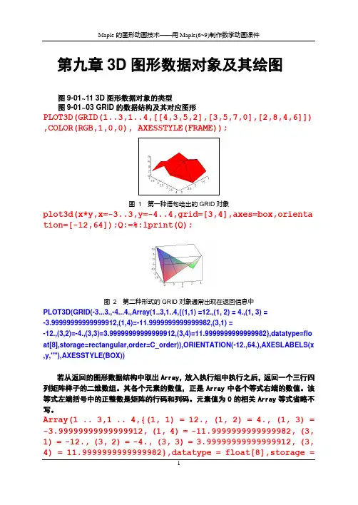
第九章3D图形数据对象及其绘图图9-01~11 3D图形数据对象的类型图9-01~03 GRID的数据结构及其对应图形PLOT3D(GRID(1..3,1..4,[[4,3,5,2],[3,5,7,0],[2,8,4,6]]) ,COLOR(RGB,1,0,0), AXESSTYLE(FRAME));图 1 第一种语句给出的GRID对象plot3d(x*y,x=-3..3,y=-4..4,grid=[3,4],axes=box,orienta tion=[-12,64]);Q:=%:lprint(Q);图 2 第二种形式的GRID对象通常出现在返回信息中PLOT3D(GRID(-3...3.,-4...4.,Array(1..3,1..4,{(1,1) =12.,(1, 2) = 4.,(1, 3) =-3.99999999999999912,(1,4)=-11.9999999999999982,(3,1) =-12.,(3,2)=-4.,(3,3)=3.99999999999999912,(3,4)=11.9999999999999982},datatype=flo at[8],storage=rectangular,order=C_order)),ORIENTATION(-12.,64.),AXESLABELS(x ,y,""),AXESSTYLE(BOX))若从返回的图形数据结构中取出Array，放入执行组中执行之后，返回一个三行四列矩阵样子的二维数组。

其各个元素的数值，正是Array中各个等式右端的数值。

该等式左端括号中的正整数是矩阵的行码和列码。

元素值为0的相关Array等式省略不写。

Array(1 .. 3,1 .. 4,{(1, 1) = 12., (1, 2) = 4., (1, 3) = -3.99999999999999912, (1, 4) = -11.9999999999999982, (3, 1) = -12., (3, 2) = -4., (3, 3) = 3.99999999999999912, (3, 4) = 11.9999999999999982},datatype = float[8],storage =rectangular,order = C_order);同一个单片曲面图形，可以使用两种形式的数据结构表示它的数据对象，效果是相同的。

[转载]maple之绘图篇~by zn~原⽂地址：maple之绘图篇~by zn~作者：ctrle如何设置maple中坐标轴的格式，look for help ?tickmarks还有⼀个问题尚未解决，就是maple中legend的位置只能放在“上下左右”四个位置，能不能⾃由放置legend哎，真费解啊，期待⾼⼈解决/maple 作图选项（图像中字体、字号等的设置）选项设置格式取值范围说明adaptive adaptive= true还有false⾃适应，取消axes axes=normal frame, boxed,normal, none坐标轴设置，四种axesfont axesfont=[family,style,size]参看plot,options 设置刻度线标号字形color color=n参看plot,color设置图象颜⾊coords coords=name polar (极坐标)参看plot[coords]选择作图所⽤坐标系discont discont=false还有true是否在间断点⽤垂直线连接filled filled=false还有true是否在图象和x轴之间填充font font=[family,style,size ]参看plot,options 设置图象中⽂字部分的字形labels labels=[x,y]　标记坐标轴labeldirections labeldirections=[x,y]horizontal, vertical设置坐标轴的⽅向Labelfont labelfont=[family,style,size ]　设置坐标轴标记的字形legend legend=s s是元素与曲线条数相同的表加⼊图例linestyle linestyle=11-4对应实线,点线,虚线和点划线设置图象线的类型numpoints numpoints =50正整数设置作图区间的分点数resolution resolution=200正整数设置图象的⽔平分辨率sample sample =[x1,..,xk]⾃变量的取值选定作图是必须取的点scaling scaling=unconstrained constrained x轴与y轴单位的⽐style,style=line point, 参看plot,options设置图象点之间的连接⽅式symbol symbol=point box, cross, circle设置图象中点的类型symbolsize symbolsize=10正整数,单位：吋/72设置图象中点的⼤⼩thickness thickness=01, 2, 3设置图象中线的厚度tickmarks tickmarks =[m,n]正整数或default设置图象中坐标轴标号个数title title =”…n…”n⽤作题⽬中的换⾏作图象标题titlefont titlefont[family,style,size ]参看plot,options 设置图象标题⽂字字形view view =[x1..x2, y1 ..y2]　设置图象坐标选取范围xtickmarks xtickmarks =n正整数设置横坐标轴标号个数Plotting Options (English help)The style of the displayed graph may be controlled with a number of plotting options embedded in the plotting command. For instance the command> plot3d(x^2+y^2, x=-1..1, y=-1..1, style=wireframe, grid=[15,15]);displays the graph in wireframe using a 15x15 grid. (Dynagraph's default action is to display the graph as a solid surface using an (invisible) grid of 25x25.)All options take the form option=value. These can be supplied to the plotting command in any order, separated by commas. The following list describes all the options recognized by dynagraph. These form a subset of options available in Maple. The listing below has been obtained mostly by cut-and-paste from Maple's online help. The options pointsize and the option values x_gridlines and y_gridlines are specific to dynagraph and do not exist in Maple.Option values which are keywords, such as WIREFRAME or HELVETICA can be typed either in all uppercase or all lowercase. Therefore axesfont=[HELVETICA,10] and axesfont=[helvetica,10] are equivalent. In the listing below only the uppercase variants are shown.Alphabetical listing of all optionsaxes=fThis option specifies how the axes are to be drawn, where f is one of BOXED, NORMAL, FRAME, and NONE.Default: axes=NONERemark: In this release of dynagraph all axes options other than NONE are treated as synonymous with BOXED. This may be fixed in future releases.axesfont=lThis option defines the font for the labels on the tick marks of the axes, specified in the same manner as font.Default: axesfont=[HELVETICA,10]color=colornamePrescribes a solid color for the object. Colorname may be any color name recognizable by the X server, such as "red" or "MidnightBlue", or an RGB specification such as "#009000". It must be quoted if it contains non-alphanumericcharacters. For the convenience of our continental friends, colour is provided as a synonym to color.contours=nThis option specifies the number of contours in a contour plot.Default: contours=10coords=cThis option specifies the coordinate system to be used, where c is one of CARTESIAN, SPHERICAL, CYLINDRICAL,Z_CYLINDRICAL.Default: coords=CARTESIANfont=fontspecThis option defines the font for text objects in the plot. Fontspec is a list of the form [family,style,size], where family is one of TIMES, COURIER, HELVETICA, and SYMBOL. For TIMES, style may be one of ROMAN, BOLD, ITALIC or BOLDITALIC. ForHELVETICA and COURIER style may be omitted or select one of BOLD, OBLIQUE, or BOLDOBLIQUE. SYMBOL does not accepta style option. The final value, size, is the point size to be used.Default: font=[HELVETICA,10]grid=[m,n]This option specifies the dimensions of the rectangular grid to use to represent a surface.Default: grid=[25,25]gridstyle=xThis option specifies the type of mesh which is drawn to represent the surface. The value of x is one of RECTANGULAR, TRIANGULAR, X_GRIDLINES, Y_GRIDLINES. (XY_GRIDLINES is also provided as a synonym for RECTANGULAR.) Note that these options set the mesh style but do not cause the mesh to be drawn. The drawing of the mesh is determined by the value of the style option described below.Default: gridstyle=RECTANGULARlabelfont=lThis option defines the font for the labels on the axes of the plot, specified in the same manner as font.Default: labelfont=[HELVETICA,12]labels=[x,y,z]This option specifies labels for the axes. The values of x, y, and z must be strings. The default label for the x and y axesare the names of the variables for the x and y axes and no label on the z axis. Labels are shown only when thecoords=CARTESIAN is in effect.linewidth=nSame as thickness=nnumpoints=nWhen plotting a surface this option specifies the minimum total number of points to be generated (default 625 = 25^2).Plot3d will use a rectangular grid of dimensions ~= sqrt(n). When plotting a spacecurve or a tube, this option specifies the number of points to use along the curve or along the axis of the tube. The default is 60.orientation=[longitude,colatitude]This option sets the viewing position at a point at infinity along the ray given by the spherical coordinates(longitude,colatitude), looking towards the origin.Default: orientation=[45,45]pointsize=nThis option defines the size (in pixels) of points drawn in the plots. n should be an integer from 0 to 10. 0 selects the default pointsize.Default: pointsize=3scaling=sThis option specifies whether the surface should be scaled so that it fits the screen with axes using a relative orabsolute scaling, where s is either UNCONSTRAINED or CONSTRAINED. The dynagraph graphics window is initially set to scaling=CONSTRAINED. The user may toggle the CONSTRAINED/UNCONSTRAINED button at will. Subsequent graphs will obey the button's setting unless specified otherwise on the command line.shading=sThis option specifies how the surface is colored, where s is one of XYZ, XY, Z, ZGREYSCALE, ZHUE, NONE.Default: shading=XYZstyle=sThis specifies how the surface is to be drawn, where s is one of POINT, HIDDEN, PATCH, WIREFRAME, CONTOUR,PATCHNOGRID, PATCHCONTOUR, or LINE.Default: style=PATCHNOGRIDRemark: LINE is synonymous with WIREFRAMEthickness=nThis option defines the thickness (in pixels) of lines in the plots. n should be an integer from 0 to 10. 0 selects the default thickness.Default: thickness=1tickmarks=[l,n,m]This option specifies reasonable numbers no less than l, n and m should be marked along the x-axis, y-axis, and z-axis, respectively. Each tickmarks value must be a positive integer or zero, in which case no tickmarks will drawn on the corresponding axis.Default: tickmarks=[5,5,5]title=tThis option specifies a title for the plot. The value of t must be a string. The two-character sequence n (that is, abackslash followed by n) acts as a line break within the title string, thus making multi-line titles possible. Each line of a multi-line title is horizontally centered within the window.Default: no titletitlefont=lThis option defines the font for the title of the plot, specified in the same manner as font.Default: titlefont=[HELVETICA,BOLDOBLIQUE,14]tuberadius=rThis sets the radius of the tube in a tubeplot.Default: tuberadius=1.0tubepoints=nThis sets the number of points to use for drawing each cross-section of a tubeplot. Note that the circular cross section will appear to have only n-1 equally-spaced points on its circumference, because the first and last points coincide.Default: tubepoints=16view=zmin..zmax or view=[xmin..xmax,ymin..ymax,zmin..zmax]This option indicates the minimum and maximum coordinates of the surface to be displayed on the screen.Default: displays the entire surface/~rouben/dynagraph/index.html。

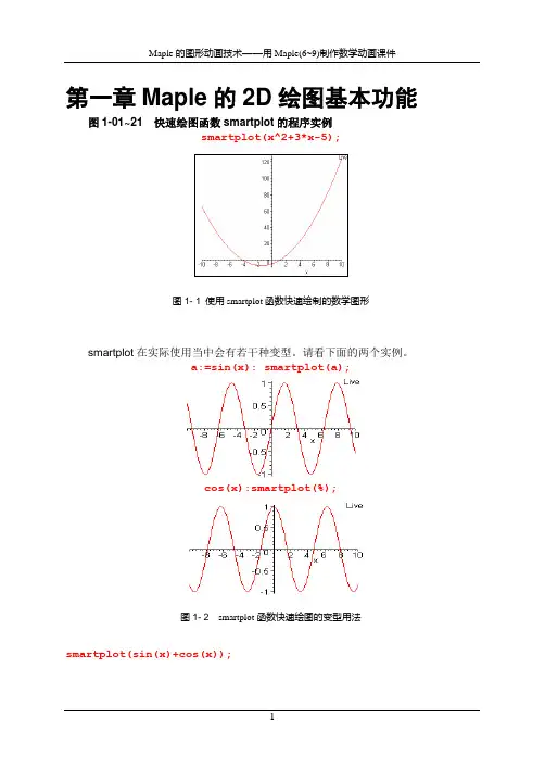
第一章Maple的2D绘图基本功能图1-01~21 快速绘图函数smartplot的程序实例smartplot(x^2+3*x-5);图1- 1 使用smartplot函数快速绘制的数学图形smartplot在实际使用当中会有若干种变型。

请看下面的两个实例。

a:=sin(x): smartplot(a);cos(x):smartplot(%);图1- 2 smartplot函数快速绘图的变型用法smartplot(sin(x)+cos(x));图1- 3 三角函数的smartplot smartplot((x^3)/7-2*x^2+15);图1- 4 多项式函数的smartplotsmartplot(sqrt(x));图1- 5 算术平方根函数的smartplot smartplot(2^x);图1- 6 指数函数的smartplotsmartplot(arctan(x));图1- 7 反正切函数的smartplot smartplot(abs(x));图1- 8 绝对值函数的smartplot smartplot(abs(x)*sin(x));图1- 9 含有绝对值符号初等函数的smartplot smartplot(ceil(x));图1- 10 内置函数ceil的smartplotsmartplot(round(x));图1- 11 内置函数round的smartplot smartplot(frac(x));图1- 12 内置函数frac的smartplot smartplot(cos(t),sin(t));图1- 13 同一自变量的函数set smartplot(cos(x),sin(y));图1- 14 不同变量的函数set smartplot(tan(x),y^2);图1- 15 以横轴做x轴的smartplot smartplot(y^2,tan(x));图1- 16 以纵轴做x轴的smartplot smartplot(x^2+y^2=64);图1- 17 代数隐函数的smartplot smartplot(abs(x-2)+abs(y-2)=7);图1- 18 含绝对值隐函数的smartplot f:=x->piecewise(x>=0 and x<3,x^3-8,x<0 and x>=-3,x,9<x^2,5):f(x);⎧⎩⎪⎪⎪⎪⎪⎪⎨ - x 38 and ≤ -x 0 < x 3x and < x 0 ≤ - - 3x 05 < 9x2smartplot(f(x));图1- 19 编程自定义函数的smartplotsmartplot([cos(t),sin(t)]);图1- 20 一对函数组成的list 被绘制成两条曲线smartplot([[1,1],[2,2]]);Error, smartplot expects its 1stargument, f, to be of type {algebraic, algebraic = algebraic, {set, list} ({algebraic, algebraic = algebraic})}, but received [[1, 1], [2, 2]]smartplot(y-2*x<1);smartplot(cos(x),sin(x),coord=polar);图1- 21 设置项coord=polar被理解为方程y=z型表达式图1-33~38 基本绘图函数plot()的程序实例plot((x^2)/3+x-4,x=-8..5);图1-33 只有描绘范围设置的plotf:=x->piecewise(x>=0 and x<3,x^3-8,x<0 and x>=-3,x,9<x^2,5): plot(f(x),x=-5..5,view=[-8..8,-15..25] );图1-34 描绘范围和显示范围各司其职plot([x^2,x^2+30*x*sin(x)],x=-6*Pi..6*Pi);图1-45 单元函数list的plotplot({sin(x),cos(x),sin(x)-cos(x)},x=0..2*Pi,y=-1.5..1.5);图1-36单元函数set的plotplot([seq(sin(5*t)+n*cos(t),n=-5..5)],t=0..Pi);图1-37 单元函数list of seq的plotplot(sin(t),t=-infinity..infinity,y=-1.2..1.2);图1-38 “无穷区间”上单元函数的plot图1-39~42 绘制参数方程曲线的程序实例plot([2*cos(t),sin(t),t=0..2*Pi]);图1-39 单条参数曲线plot([sin(4*t),sin(3*t),t=0..4*Pi],x=-2..2,y=-1.5..1.5);图1-40 参数曲线图中xy范围可控制显示范围plot([[cos(t),sin(t),t=0..2*Pi],[sin(2*t),sin(3*t),t=0..4*Pi] ]);图1-41 两条参数曲线的ploteq1:=[sin(2*t),sin(3*t),t=0..4*Pi]:eq2:=[cos(t),sin(t),t=0..2 *Pi]:plot([eq1,eq2]);图1-42 两条参数曲线plot的另一种语句图1-43~55 绘制点列或折线的程序实例plot([[1.5,1],[2,2],[0.4,1.4]],view=[0..2.5,0..3],style=POINT );图1-43 不连线的点列图1-44 连线的点列plot([[3,2],[2,3],[0,1],[2,0],[3,2]]);图1-45 封闭折线n:=5:plot([[seq([cos(2*Pi*i/n),sin(2*Pi*i/n)],i=0..n)]]);图1-46 用seq给出的点列（不联线）图1-47 用seq给出的点列（联线）plot([[seq([cos(2*Pi*2*i/n),sin(2*Pi*2*i/n)],i=0..n)]]);图1-48 用seq给出的点列（隔点联线）孤立点的图形是特例，但有特殊用途。

第三章2D图形数据对象及其绘图图3. 1 Maple的绘图机理图3. 2 图形数据对象的组成图3-03~04 用PLOT法给数据对象绘图编写一批（8个）图形数据对象。

对前四个，侧重注意它们的对象名称和对象信息；对后四个，注意局部信息。

O1:=POINTS([0,0],SYMBOL(DIAMOND,28)):O2:=CURVES([[3.1416,0],[0,3.1416]],[[-4,0],[0,-4]],STYLE(POINT),SYMBOL(CIRCLE,36),COLOR(RGB,0,0,1)):O3:=CURVES([[3,0],[0,3]],STYLE(LINE),LINESTYLE(4),THICKNESS(3),COLOR(RGB,1,0,1)):O4:=POLYGONS([[-4,0],[-4,-4],[0,-4]],COLOR(HUE,0.5)):O5:=TEXT([0,0],"Yuandian",ALIGNBELOW,FONT(TIMES,BOLD,12),COL OR(RGB,1,0,0)):O6:=TEXT([0+.5,3.1416],"p",ALIGNABOVE,ALIGNRIGHT,FONT(SYMBOL ,12)):O7:=TEXT([3.1416+.5,0+.5],"p",ALIGNABOVE,ALIGNRIGHT,FONT(SYM BOL,12)):O8:=TEXT([-3,-3],"Sanjiaoxing",FONT(TIMES,BOLD,12)):下图中的8个小图形，是将前述8个命令逐一添加到组合图形中去的结果。

每一小图，都是前一小图又加入新对象的结果。

图3. 3 把前述8个数据对象逐一添加到图形中去若想把前面分别写出的8个数据对象O1~O8放在一个图中描绘，就可如下处理。

这里我们给图形的整体添加了7个设置选项（都属于表1）。

Maple⼆维曲线图命令介绍
Maple⼆维曲线图命令介绍
Maple作图的功能很强⼤且界⾯简单直观，能够对图形进⾏修改。

并且Maple作图可以作出平⾯图也可以作出⽴体图，下⾯介绍⼀些常见的Maple⼆维曲线图的命令。

参数⽅程曲线：
plot([x(t),y(t),t=t1..t2],x=a..b,y=c..d,选项)；
动画曲线：
动画曲线不是基本作图命令，必需先调⼊图形包，才能运⾏。

Aninate(f(x,t),x=a..b,t=t1..t2，选项)；其中t为参数
当点击动画图后，会显⽰动画按钮，由按钮控制动画。

极坐标：
注：如果函数由f:=proc(x)定义，作图由plot(f)或plot(f,a..b)或plot(f(x),x=a..b)
多边形及填⾊：polygon([顶点坐标]，颜⾊)要调⽤图形⼯具包
曲边梯形⾯积：y=sin（x），y=0，x=π/2所围图形⾯积。

隐函数图：implicitplot(⽅程，范围，选项)；
注：⼆元⽅程为平⾯曲线，没有等号默认为等于0。

以上内容向⼤家介绍了常见的Maple⼆维曲线图的命令及调⽤格式，Maple不仅可以绘制⼆维图形，三维也可以。

1 二维图形制作Maple所提供的二维绘图指令plot可以绘制二维的函数图、参数图、极坐标图、等高线图、不等式图，等等. 这些绘图指令有些已经内嵌在其核心程序里, Maple启动时即被装入，直接调用函数命令即可，有些则需要使用with(plots)调用plots函数库才能完成.1.1 基本二维绘图指令plot (f(x), x=xmin .. xmax);plot (f(x), x=xmin .. xmax, y=ymin .. ymax);plot ([f1(x), f2(x), …], x=xmin .. xmax);plot (f(x), x=xmin .. xmax, option);其中，xmin..xmax为x的变化范围，ymin..ymax为y(即f(x))的变化范围. option选项参数主要有：axes：设定坐标轴的显示方式, 一般有FRAME(坐标轴在图形的左边与下面)、BOXED(坐标轴围绕图形)、NORMAL(一般方式显示)或NONE(无)color：设定图形所要涂的颜色(可选用也可自设)coords：指定绘图时所用的坐标系(笛卡尔坐标系(cartesian，默认)、极坐标系(polar)、双极坐标系(bipolar)、logarthmic(对数坐标系)等discont：设定函数在不是否用线段连接起来(discont=true则不连接, 默认是discont=false) labels：设定坐标轴的名称(labels=[x, y], x与y分别为x与y坐标轴的名称)linestyle：设定所绘线条的线型(linestyle=n, n为1是实线, 2为点, 3为虚线, 4为虚线与点交错)numpoints：设定产生一个函数图形所需的最少样点scaling：设置x与y轴的比例(unconstrained非约束，constrained约束，比例为1:1)style：设定图形的显示样式(LINE(线形)、POINT(点)、PA TCH(显示多边形与边线)、PA TCHNOGRID(只显示色彩而无边界)symbol：设定点的格式(主要有BOX(方块)、CROSS(十字)、CIRCLE(圆形)、POINT(点)、DIAMOND(菱形)等几项)thickness：设定线条的粗细(0、1、2、3几种参数, 数值越大线条越粗)tickmarks：设定坐标轴刻度的数目(设定tickmarks=[m, n], 则x轴刻度为m, y轴为n)title：定义图形的标题(要用" "把标题引起来)view：设定屏幕上图形显示的最大坐标和最小坐标，缺省是整个曲线下面通过一些实例学习：> plot(sin(1/x),x=-0.1..0.1,title="y=sin(1/x)",axes=normal);> plot(1/(2*sin(x)),x=-10..10,y=-30..30);试比较下述三图的效果:> plot(tan(x),x=-2*Pi..2*Pi);> plot(tan(x),x=-2*Pi..2*Pi, y=-5..5);> plot(tan(x),x=-2*Pi..2*Pi, y=-5..5,discont=true);(此处命令discont=true的作用是去除垂直渐近线)> plot(sin(cos(6*x))/x, x=0..15*Pi, y=-0.6..0.5, axes=NONE);> plot(Zeta(x),x=-3..3,y=-3..3,discont=true);除了绘制基本的函数图之外, plot还可绘制自定义函数的图形, 也可以同时绘制多个函数图. > f:=x->sin(x)+cos(x)^2;plot(f(x),x=0..16);> plot([sin(x),sin(x^2),sin(x^3/10)],x=-2*Pi..2*Pi);利用seq指令产生一个由函数所组成的序列, 并将此函数的序列赋给变量, 然后将函数序列绘于同一张图上.> f:=x->sin(x)+cos(x);fs:=seq(f(x)^(n-1)+f(x)^n,n=1..4):plot([fs],x=0..20);> f:=x->x*ln(x^2):g:=x->ln(x):plot({f,g},0..2,-1.5..1.5);也可以直接把seq指令放在plot里来绘出一系列的函数图.> plot([seq(f(x)^(2/n),n=1..3)],x=0..10);1.2 二维参数绘图更多情况下，我们无法把隐函数化成显函数的形式, 因而plot指令无法在二维的平面里直接绘图. 但是, 在某些情况下, 我们可以把平面上的曲线f(x, y)化成x=x(t), y=y(t)的形式, 其中t为参数(parameter). 据此即可绘图, 其命令格式如下：plot ([x(t), y(t), t=tmin .. tmax])；plot ([x(t), y(t), t=tmin .. tmax], xmin .. xmax, y=ymin .. ymax)；plot ([x(t), y(t), t=tmin .. tmax], scaling=CONSTRAINED);plot ([[x1(t), y1(t), t1=t1min .. t1max], [x2(t), y2(t), t2=t2min .. t2max],…]);> plot([t*exp(t),t,t=-4..1],x=-0.5..1.5,y=-4..1);> plot([sin(t),cos(t),t=0..2*Pi]);> plot([sin(t),cos(t),t=0..2*Pi],scaling=CONSTRAINED);上述两上语句都是绘制圆的命令, 但由于后者指定的x、y坐标的比例为1:1, 所以才得到了一个真正的圆, 而前者由于比例不同, 则像个椭圆. 下面则是内摆线的图形：> x:=(a,b)->(a-b)*cos(t)+b*cos((a-b)*t/b);> y:=(a,b)->(a-b)*sin(t)-b*sin((a-b)*t/b);当a=1, b=0.58时，(x(a,b), y(a,b))图形绘制命令为：> plot ([x(1,0.58), y(1,0.58), t=0..60*Pi], scaling=CONSTRAINED);再作a, b取其它值时的情形：> plot([x(2,1.2),y(2,1.2),t=0..6*Pi],scaling=CONSTRAINED);> plot([x(2,8),y(2,8),t=0..16*Pi],scaling=CONSTRAINED);> plot([x(2,12),y(2,12),t=0..16*Pi],scaling=CONSTRAINED);下面再看同时绘制多个图形的情形.> plot([[cos(3*t),sin(2*t),t=0..2*Pi],[sin(t),cos(3*t),t=0..2*Pi]]);1.3 数据点绘图如果所绘的图形是间断性的数据, 而不是一个连续的函数, 那么我们可以把数据点绘在x-y 坐标系中, 这就是所谓的数据点绘图. 其命令格式如下：plot([[x1, y1], [x2, y2], …], style=point);plot([[x1, y1], [x2, y2], …] );> data1:=seq([2*n,n^3+1],n=1..10):plot([data1],style=point);> data2:=seq([n,1+(-1)^n/n],n=1..15):plot([data2],style=point,view=[0..20,0..2]);> data3:=seq([t*cos(t/3),t*sin(t/3)],t=1..30):plot([data3],style=point);1.4 其它坐标系作图由于所研究的问题的特殊性，常常需要选用不同的坐标系, 在Maple中除笛卡尔坐标系(cartesian, 也称平面直角坐标系, 默认)外，还提供了polar(极坐标系)、elliptic(椭圆坐标系)、bipolar(双极坐标系)、maxwell(麦克斯韦坐标系)、logarithmic(双数坐标系)等14种二维坐标系，其中最常用的是极坐标系。

第七章Maple的3D图形基本功能图7-01~06快捷绘图函数smartplot3d的运用smartplot3d(x^2+y^2);lprint(%);图1smartplot3d直接返回的图形和数据结构smartplot3d(abs(x)+abs(y)+abs(z)=4);lprint(%);图2smartplot3d还可以接受非初等函数的隐函数方程smartplot3d(x^2+y^2,x*y);lprint(%);图3smartplot3d可以接受多个表达式并可分别做交互式设置利用函数smartplt3d还可以绘制自定义的“分区函数”的图形。

M:=(x,y,z)->piecewise(y>0and x>0,1,-1);M(x,y,z);smartplot3d(M(x,y,z));lprint(%);图4利用smartplot3d绘制“分区函数”的图形（做过交互式设置）smartplot3d函数具有multyple功能，因而可以绘制曲面族的图形。

smartplot3d(seq(x^2+y^2+125*i,i=1..4));图5利用smartplot3d函数的multyple功能绘制曲面族的图形可以把smartplot3d函数返回的图形数据结构拷入一个执行组，并添加一些plot设置选项，再次执行。

INTERFACE_SMARTPLOT3D([x^2+y^2,x,y,_NoZ],style=LINE,a xes=frame,color=blue);lprint(%);图6把图１的返回数据拷入一个执行组，并添加一些设置选项，再次执行的结果图73D图形窗口图83D图形工具栏的第一组图93D图形工具栏的第二组图10各钮对应的图形样式图113D图形工具栏的第三组图12不同样式的坐标架图13Style级联菜单图14Color级联菜单INTERFACE_SMARTPLOT3D([x^2+y^2-z^2=1,x,y,z],color=cya n,view=[-3..3,-3..3,-2..2]);图15按着命令语句生成的图形图16鼠标指向图形，颜色变得灰暗图17选中color命令引出级联菜单图186条命令的不同着色效果图19使用曲面样式选项和颜色选项分别设置的实例图20坐标架的四种样式图21Ranges命令可确定各个坐标轴的显示范围图22Projection级联菜单图23不同的投影类型图24绘制3D图形的子菜单命令图25从返回信息中选定一个三元表达式，绘制快捷图形图26从返回信息中选定一个二元表达式，绘制3D快捷图形图27从返回信息中选定一个二元表达式，绘制2D快捷图形图28从返回信息中选定一个一元表达式，绘制2D快捷图形图29从返回信息中选定一个一元表达式，绘制3D快捷图形图30 6.0中选定单变量表达式只能绘制2D图形图317.0中选定单变量表达式还能绘制3D图形图7-32~34plot3d的调用语句plot3d(x*exp(-x^2-y^2),x=-2..2,y=-2..2,color=green);图32用plot3d绘制单片曲面plot3d([sin(x)*cos(y),sin(x)*sin(y),cos(x)],x=0..Pi/2, y=0..x);图33用plot3d绘制参数曲面plot3d([x,y,sqrt(4-x^2-y^2)],x=-1.999..1.999,y=-sqrt( 4-x^2)+1/920..sqrt(4-x^2),grid=[15,35]);图34参数曲面，变量y的范围界线是x的函数图7-35~41plot3d的调用语句的设置选项plot3d(1,t=0..2*Pi,p=0..Pi,orientation=[50,70],scalin g=constrained,axes=box);plot3d(1,t=0..2*Pi,p=0..Pi,coords=cylindrical,scaling =constrained,orientation=[50,70],axes=box);plot3d(1,t=0..2*Pi,p=0..Pi,coords=spherical,scaling=c onstrained,orientation=[50,70],axes=box);图35表达式“1”在三种坐标系（直角系、圆柱系、球面系）中的图形plot3d(v,u=0..2*Pi,v=-1..1,title=`CONE`,scaling=uncon strained,orientation=[50,70],axes=box);plot3d(v,u=0..2*Pi,v=-1..1,coords=cylindrical,title=` CONE`,scaling=unconstrained,orientation=[50,70],axes= box);plot3d(v,u=0..2*Pi,v=-1..1,coords=spherical,title=`CONE`,scaling=unconstrained,orientation=[50,70],axes=bo x);图36表达式“v ”在三种坐标系（直角系、圆柱系、球面系）中的图形plot3d(u,u=0..2*Pi,v=-2..2,title=`CONE`,scaling=uncon strained,orientation=[50,70],axes=box);plot3d(u,u=0..2*Pi,v=-2..2,coords=cylindrical,title=`CONE`,scaling=unconstrained,orientation=[50,70],axes=box);plot3d(u,u=0..2*Pi,v=-2..2,coords=spherical,title=`CO NE`,scaling=unconstrained,orientation=[50,70],axes=bo x);图37表达式“u ”在三种坐标系（直角系、圆柱系、球面系）中的图形plot3d((1.3)^x*sin(y),x=-1..2*Pi,y=0..Pi,style=patch);plot3d((1.3)^x*sin(y),x=-1..2*Pi,y=0..Pi,coords=cylin drical,style=patch);plot3d((1.3)^x*sin(y),x=-1..2*Pi,y=0..Pi,coords=spher ical,style=patch);图38表达式“(1.3)^x*sin(y)”在三种坐标系（直角系、圆柱系、球面系）中的图形范围的端值可以使用变量在某些情况下，范围的端值可以使用变量。

利用数学软件MAPLE进行曲线拟合的操作方法
一、安装MAPLE（我这里有个镜像安装文件MAPLE 15，约400M，需要的可以来拷）
二、启动MAPLE，主界面如下：
三、点击“工具”→“助手”→“曲线拟合”
弹出如下界面，填入数值，第一列是X的值，第二列是Y的值，
然后点击按钮“Fit”，弹出如下界面：
四、点击上图中红色部分按钮“Plot”，即可生成曲线，如下图所示：
图中，
区域2：调节曲线的圆滑度，数值8最圆滑最贴近；
区域3：可以选择进行几次多项式的拟合，如二次、三次、四次等等，注意表达式的书写方式，如三次表达式为a*x^3 + b*x^2 + c*x + d，四次表达式为a*x^4 + b*x^3 + c*x^2 + d*x +e，以此类推；
区域4：显示所指定次数多项式最终拟合曲线的函数表达式。

（此式便可以用来计算刘星老师所布置的不同温度下的吉布斯自由能）。

默认显示最贴近的拟合函数。