Rfmap使用文档

rf测试用例格式-概述说明以及解释1.引言1.1 概述概述在软件测试领域，RF测试用例格式是一种关键的工具，用于确保软件系统的质量和稳定性。

RF测试用例格式是指对软件系统进行功能测试时所需编写的测试用例的规范格式。

它包括了测试用例的名称、目的、前提条件、步骤、预期结果等内容，以便测试人员能够清晰地了解测试的目的和过程。

通过使用统一的RF测试用例格式，测试团队可以更加系统地编写和管理测试用例，提高测试效率和质量。

同时，RF测试用例格式也有助于提高团队间的沟通和协作，减少测试过程中的偏差和误解。

本文将详细探讨RF测试用例格式的重要性、具体要点以及实践中的应用建议，希望能够帮助读者更好地理解和运用RF测试用例格式，提高软件测试工作的效率和效果。

1.2 文章结构文章结构是指文章整体的组织框架和章节安排。

在本文中，我们采用了引言、正文和结论三个主要部分来组织文章结构。

- 引言部分会简要介绍文章的主题，包括概述、文章结构和目的，为读者提供对整篇文章的整体了解。

- 正文部分包括了什么是RF测试用例格式、RF测试用例格式的重要性以及RF测试用例格式的具体要点，详细讨论了RF测试用例格式的相关知识和重要性。

- 结论部分总结了RF测试用例格式的作用，并提出了在实践中应用RF测试用例格式的建议，同时展望了未来发展方向，为读者提供了对RF 测试用例格式的更深入的理解和展望。

1.3 目的RF测试用例格式的主要目的是为了规范和统一测试用例的编写和实施过程，以提高测试效率和准确性。

通过使用统一的格式，可以使测试用例更容易被理解和执行，并且可以帮助测试人员更好地掌握测试的范围和目标。

另外，RF测试用例格式的制定也是为了方便测试结果的记录和分析，从而推动测试过程的持续改进和提升。

最终的目的是确保产品的质量和稳定性，提升用户体验和满意度。

2.正文2.1 什么是RF测试用例格式在软件测试中，测试用例是用来验证软件系统是否符合需求和设计规范的重要工具。

全站仪的使用坐标测量操作步骤1.2.为安全起见,在进行外业测量之前,应预先充足电池,准备好已充满电的备用电池;按“MENU”键进入“菜单”,由主菜单选择“1数据采集”进入“选择文件”界面;文件主要功能是管理、存储所采集的数据;文件可直接按“F1输入”创建一个新文件名,文件名可以是数字或字母,建议以当天日期或当地地名建文件;文件也可按“F2调用”查找已经存在仪器当中的文件,当文件被选定时,在该文件名的左边显示一个符号“”然后“回车”;文件选定后,进入“数据采集”界面;选择“1设置测站点”进入设置测站点界面;“F1输入”测站点点号、编码一般不设、仪器高,然后按“F4测站”进入“测站点”界面;按“F3坐标”输入测站点坐标,然后“F4回车”,再按“F3记录”选择“F4是”,返回“数据采集”界面;这时测站点设置完毕;若内存中已有测站点坐标也可直接按F2调用,检核无误后选择“是”,“F3记录”;在“数据采集”界面中选择“2设置后视点”进入设置方位角界面;输入后视点点号、镜高,然后按“F4后视”进入“后视点”界面,按“F2调用”坐标或按“F3 NE/AZ”直接输入坐标,然后“F4回车”返回到设置方向角,将望远镜瞄准后视点,按“F3测量”再按“F3坐标”,测完后方向角即被设置也可以直接按F1角度,出现坐标方位角,对准后视点,选择是,然后返回“数据采集”界面;6.在“数据采集”界面中选择“3测量点”,输入待测点点号,设置镜高,然后按“F3测量”“F3坐标”,“F4是”存储数据;放样操作步骤：1.按“MENU”键进入“菜单”,由主菜单选择“2放样”进入“选择文件”界面;选择一个坐标数据文件,回车,进入“放样”;“1设置测站点”按“F2调用或F3坐标,直接输入”,“F4”确认2.“2设置后视点”按“F2调用”坐标或按“F3 NE/AZ”直接输入坐标,然后“F4回车”返回到设置方向角,将望远镜瞄准后视点,“F4是”3.“3设置放样点”进入,按“F2调用”或F3坐标直接输入,“F4确认”,按“F1距离”,将DHR调到0°00′00″即表明放样方向正确,锁定望远镜,指挥跑杆员走到该确定的方向,按“F3距离”测距,4. 当DHD=0时则表明放样点测设完成;。

全网性RF优化分析快捷方法案例电子地图-TAB图层制作深圳齐普生网络优化部Shenzhen Chips Information S&T Co.,Ltd2011-01-02目录1概述 (2)2分析步骤简介 (2)3原理简介 (2)4优化分析工具使用说明 (2)4.1E都市电子地图截取 (2)4.2使用图形图像处理软件对图片进行合并 (6)4.3图片制作TAB图层 (9)5分析案例 (10)6附件 (11)6.1电子地图一把抓软件 (11)1 概述RF调整在所有的无线网络优化中是最重要的手段之一，高效、快速的RF分析方法非常重要，下面对RF优化分析提供一种快速、高效的方法。

在一个项目启动，项目人员对本地的地理环境不是很熟悉，对站点周边无线覆盖环境情况不是很熟悉的时候，可以通过对网络上专业的电子地图进行截取，在Mapinfo软件中以地图的方式呈现，对地理环境站点小区周边存在的信号阻挡、反射、拐角效应，针尖效应了如指掌，提高工作效率。

2 分析步骤简介第一步：通过电子地图一把抓软件将E都市电子地图进行多图抓取；第二步：通过图形图像软件进行整图合并；第三步：在Mapinfo中对图片进行3点定位，生成TAB图层；第四步：制作好后，进行分析；3 原理简介电子地图一把抓：使用电子地图一把抓软件，抓取多屏图片，软件可以智能截取合并；Photoshop：；使用Photoshop软件对多图片进行合并处理，生成城市完整电子地图；Mapinfo：使用Mapinfo中对图片3点定位，确定经纬度，生成TAB图层。

4 优化分析工具使用说明4.1 E都市电子地图截取图片使用电子地图一把抓软件。

图1运行MapCap_LZW.exe打开软件运行抓图向导。

图2电子地图一把抓运行抓图向导设置截取区域：运行抓图向导后，此时程序主窗口将会隐藏,出现区域设定窗口。

切换到目标地图软件，调整区域设定窗口的大小和位置，使得该窗口正好完全覆盖目标地图软件中的地图窗口。

MapInfo常规使用方法使用M apInfo Pro fessi o nal第一部分MAPINFO桌面地图系统简介一.概述GIS出现20年,成为比较成熟的技术。

80S以来,商品软件如ARC/INFO,CICAD,MGE(Intergraph)等, GIS走出实验室进入实用。

用户中有大量的如数据可视化,地理分析等的需求,但传统GIS产品的价格高,专业性强,应用平台高,界面复杂,普通用户难以完成开发。

而MAPINFO结合数据库与电子地图,适合PC机运行,易于使用和二次开发,是一种桌面地图信息系统。

MAPINFO总部在美国,用户遍及58个国家,有6种语言的版本。

应用于市政管理,市场策划与规划,土地与自然管理,交通运输,保险服务,通讯业务,治安,教育,经济,银行等。

MICROSOFT与MAPINFO协议, OFFICE组件及EXCEL中融入基本的桌面地理信息功能。

95年北京成立MAPINFO中国有限公司,在上海,广州,成都等地设立分公司。

二.MAPINFO软件1.总体介绍85%以上的数据具有地理信息,而表格式和文字式的数据表达形式不能把大量的信息清晰地表现在人们面前,如将各种数据放在地图上表示出来,辅以地理分析,可使它们之间的关系趋势一目了然。

3.0 FOR WIN 的环境要求CPU 386以上,内存4M-8M,VGA以上显示器,软件4.5M空间,样本数据7.5M空间.WIN3.1以上。

地图输入及编辑1)数字化仪输入地图(如利用美DTC公司的VTI接口软件,MAPINFO可与流行的SUMMAGRAGHICS ,CALCOMP等200多种数字化仪连接)2)通过其它绘图工具绘制地图(支持标准的DXF格式输入,可ACAD,COREL DRAW通过等输入地图,再输出成DXF文件,MAPINFO 再读入DXF文件)3)光栅图象(RAST ER IMAGE)输入(支持BMP,GIF,J PEG,PCX,SPOT[卫星航空照片位图],TGA,TIFF格式,输入后,可用MAPINFO的作图工具在其上作图,编辑,再存成单独的矢量地图层,也可把光栅图象作为底图,以增强图面效果)作图工具和命令包括:直线,折线,圆/椭圆,多边形,圆弧,矩形/方形,文本;改变状态,增加节点;各种数据的增删改等编辑命令。

Arc Map的基本使用介绍Arc Map是一款强大的地理信息系统软件，广泛应用于地理空间数据的管理、分析和可视化。

本文将详细介绍Arc Map的基本使用，包括软件的安装与配置、数据的导入与管理、地图的创建与编辑、空间分析等方面。

安装与配置1.下载Arc Map安装程序；2.运行安装程序，按照提示完成安装；3.打开Arc Map，进入软件的设置界面；4.配置软件的默认存储路径、界面语言等参数。

数据的导入与管理导入数据1.点击”添加数据”按钮，选择要导入的数据文件；2.在弹出的对话框中选择数据源和数据类型；3.确认导入选项，点击”确定”按钮。

管理数据1.在”目录”窗格中，右键点击数据，选择相应的管理操作；2.可以对数据进行重命名、删除、复制、移动等操作；3.可以创建数据集、数据集合、地图文档等组织数据。

地图的创建与编辑创建地图1.点击”新建地图”按钮，选择地图模板；2.设置地图的名称、坐标系统、单位等属性；3.确认设置，点击”确定”按钮。

地图的基本操作1.放大与缩小：使用放大工具或缩小工具，点击地图进行相应操作；2.平移：使用平移工具，点击并拖动地图；3.查询：使用查询工具，点击地图进行查询操作。

地图的编辑1.启用编辑：点击”编辑”菜单，选择”启用编辑”；2.选择要编辑的图层，点击”编辑工具”按钮；3.进行编辑操作，如添加、删除、移动要素等；4.保存编辑结果，点击”保存编辑”按钮。

空间分析空间查询1.选择要查询的图层，点击”查询”按钮；2.在查询对话框中设置查询条件，点击”确定”按钮；3.查询结果将以高亮显示在地图上。

缓冲区分析1.选择要进行缓冲区分析的图层，点击”缓冲区”按钮；2.在缓冲区对话框中设置缓冲区半径、单位等参数；3.确认设置，点击”确定”按钮；4.缓冲区结果将以新的图层显示在地图上。

空间统计1.选择要进行空间统计的图层，点击”统计”按钮；2.在统计对话框中选择统计字段和统计方法；3.确认设置，点击”确定”按钮；4.空间统计结果将以表格形式显示。

Package‘rfm’October14,2022Type PackageTitle Recency,Frequency and Monetary Value AnalysisVersion0.2.2Description Tools for RFM(recency,frequency and monetary value)analysis.Generate RFM score from both transaction and customer level data.Visualize therelationship between recency,frequency and monetary value using heatmap,histograms,bar charts and scatter plots.Includes a'shiny'app forinteractive segmentation.References:i.Blattberg R.C.,Kim BD.,Neslin S.A(2008)<doi:10.1007/978-0-387-72579-6_12>. License MIT+file LICENSEURL https:///rsquaredacademy/rfm,https:///BugReports https:///rsquaredacademy/rfm/issuesDepends R(>=3.2)Imports dplyr,ggplot2,ggthemes,lubridate,magrittr,RColorBrewer,rlang,stats,tibble,tidyr,utils,xplorerrSuggests covr,DT,kableExtra,knitr,rmarkdown,testthat,vdiffrVignetteBuilder knitrEncoding UTF-8LazyData trueRoxygenNote7.1.0NeedsCompilation noAuthor Aravind Hebbali[aut,cre](<https:///0000-0001-9220-9669>) Maintainer Aravind Hebbali<*************************>Repository CRANDate/Publication2020-07-2111:10:03UTC1R topics documented:rfm (2)rfm_barchart_data (2)rfm_bar_chart (3)rfm_data_customer (4)rfm_data_orders (5)rfm_heatmap (5)rfm_heatmap_data (6)rfm_histograms (7)rfm_hist_data (8)rfm_launch_app (9)rfm_order_dist (9)rfm_plot_median_recency (11)rfm_rm_plot (12)rfm_segment (13)rfm_table_customer (14)rfm_table_customer_2 (16)rfm_table_order (17)Index19 rfm rfm packageDescriptionTools for customer segmentation analysisrfm_barchart_data Bar chart dataDescriptionData for generating bar charts.Usagerfm_barchart_data(rfm_table)Argumentsrfm_table An object of class rfm_table.Examples#using transaction dataanalysis_date<-lubridate::as_date( 2006-12-31 )rfm_order<-rfm_table_order(rfm_data_orders,customer_id,order_date,revenue,analysis_date)#bar chart datarfm_barchart_data(rfm_order)#using customer dataanalysis_date<-lubridate::as_date( 2007-01-01 )rfm_customer<-rfm_table_customer(rfm_data_customer,customer_id,number_of_orders,recency_days,revenue,analysis_date)#bar chart datarfm_barchart_data(rfm_customer)rfm_bar_chart RFM bar chartDescriptionExamine the distribution of monetary scores for the different combinations of frequency and recency scores.Usagerfm_bar_chart(rfm_table,bar_color="blue",xaxis_title="Monetary Score",sec_xaxis_title="Frequency Score",yaxis_title="",sec_yaxis_title="Recency Score",print_plot=TRUE)Argumentsrfm_table An object of class rfm_table.bar_color Color of the bars.xaxis_title X axis title.sec_xaxis_titleSecondary x axis title.yaxis_title Y axis title.sec_yaxis_titleSecondary y axis title.print_plot logical;if TRUE,prints the plot else returns a plot object.4rfm_data_customer ValueBar chart.Examples#using transaction dataanalysis_date<-lubridate::as_date( 2006-12-31 )rfm_order<-rfm_table_order(rfm_data_orders,customer_id,order_date,revenue,analysis_date)#bar chartrfm_bar_chart(rfm_order)rfm_data_customer RFM customer dataDescriptionA dataset containing customer level data.Usagerfm_data_customerFormatA tibble with39,999rows and5variables:customer_id Customer id.total_amount Total amount of all orders.most_recent_visit Date of the most recent transaction.number_of_purchases Total number of transactions/orders.purchase_interval Number of days since last transaction/order.rfm_data_orders5 rfm_data_orders RFM transaction dataDescriptionA dataset containing transactions of different customers.Usagerfm_data_ordersFormatA tibble with49.6rows and3variables:order_date order datecustomer_id customer idrevenue transaction amountrfm_heatmap RFM heatmapDescriptionThe heat map shows the average monetary value for different categories of recency and frequency scores.Higher scores of frequency and recency are characterized by higher average monetary value as indicated by the darker areas in the heatmap.Usagerfm_heatmap(data,plot_title="RFM Heat Map",plot_title_justify=0.5,xaxis_title="Frequency",yaxis_title="Recency",legend_title="Mean Monetary Value",brewer_n=5,brewer_name="PuBu",print_plot=TRUE)6rfm_heatmap_dataArgumentsdata An object of class rfm_table.plot_title Title of the plot.plot_title_justifyHorizontal justification of the plot title;0for left justified and1for right justi-fied.xaxis_title X axis title.yaxis_title Y axis title.legend_title Legend title.brewer_n Indicates the number of colors in the palette;RColorBrewer is used for the color palette of the heatmap;check the documentation of brewer.pal.brewer_name Palette name;check the documentation of brewer.pal.print_plot logical;if TRUE,prints the plot else returns a plot object.Examples#using transaction dataanalysis_date<-lubridate::as_date( 2006-12-31 )rfm_order<-rfm_table_order(rfm_data_orders,customer_id,order_date,revenue,analysis_date)#heat maprfm_heatmap(rfm_order)#using customer dataanalysis_date<-lubridate::as_date( 2007-01-01 )rfm_customer<-rfm_table_customer(rfm_data_customer,customer_id,number_of_orders,recency_days,revenue,analysis_date)#heat maprfm_heatmap(rfm_customer)rfm_heatmap_data Heatmap dataDescriptionData for generating heatmap.Usagerfm_heatmap_data(rfm_table)Argumentsrfm_table An object of class rfm_table.rfm_histograms7Examples#using transaction dataanalysis_date<-lubridate::as_date( 2006-12-31 )rfm_order<-rfm_table_order(rfm_data_orders,customer_id,order_date,revenue,analysis_date)#heat map datarfm_heatmap_data(rfm_order)#using customer dataanalysis_date<-lubridate::as_date( 2007-01-01 )rfm_customer<-rfm_table_customer(rfm_data_customer,customer_id,number_of_orders,recency_days,revenue,analysis_date)#heat map datarfm_heatmap_data(rfm_customer)rfm_histograms RFM histogramsDescriptionHistograms of recency,frequency and monetary value.Usagerfm_histograms(rfm_table,hist_bins=9,hist_color="blue",plot_title="RFM Histograms",xaxis_title="",yaxis_title="Count",hist_m_label="Monetary",hist_r_label="Recency",hist_f_label="Frequency",plot_title_justify=0.5,print_plot=TRUE)Argumentsrfm_table An object of class rfm_table.hist_bins Number of bins of the histograms.hist_color Color of the histogram.plot_title Title of the plot.8rfm_hist_data xaxis_title X axis title.yaxis_title Y axis title.hist_m_label Label of the monetary value histogram.hist_r_label Label of the recency histogram.hist_f_label Label of the frequency histogram.plot_title_justifyHorizontal justification of the plot title;0for left justified and1for right justi-fied.print_plot logical;if TRUE,prints the plot else returns a plot object.ValueHistogramsExamples#using transaction dataanalysis_date<-lubridate::as_date( 2006-12-31 )rfm_order<-rfm_table_order(rfm_data_orders,customer_id,order_date,revenue,analysis_date)#histogramrfm_histograms(rfm_order)#using customer dataanalysis_date<-lubridate::as_date( 2007-01-01 )rfm_customer<-rfm_table_customer(rfm_data_customer,customer_id,number_of_orders,recency_days,revenue,analysis_date)#histogramrfm_histograms(rfm_customer)rfm_hist_data Histogram dataDescriptionData for generating histograms.Usagerfm_hist_data(rfm_table)Argumentsrfm_table An object of class rfm_table.rfm_launch_app9Examples#using transaction dataanalysis_date<-lubridate::as_date( 2006-12-31 )rfm_order<-rfm_table_order(rfm_data_orders,customer_id,order_date,revenue,analysis_date)#histogram datarfm_hist_data(rfm_order)#using customer dataanalysis_date<-lubridate::as_date( 2007-01-01 )rfm_customer<-rfm_table_customer(rfm_data_customer,customer_id,number_of_orders,recency_days,revenue,analysis_date)#histogram datarfm_hist_data(rfm_customer)rfm_launch_app Launch shiny appDescriptionLaunches shiny app.Usagerfm_launch_app()Examples##Not run:rfm_launch_app()##End(Not run)rfm_order_dist Customers by ordersDescriptionVisualize the distribution of customers across orders.10rfm_order_distUsagerfm_order_dist(rfm_table,bar_color="blue",xaxis_title="Orders",yaxis_title="Customers",plot_title="Customers by Orders",plot_title_justify=0.5,print_plot=TRUE)Argumentsrfm_table An object of class rfm_table.bar_color Color of the bars.xaxis_title X axis title.yaxis_title Y axis title.plot_title Title of the plot.plot_title_justifyHorizontal justification of the plot title;0for left justified and1for right justi-fied.print_plot logical;if TRUE,prints the plot else returns a plot object.ValueBar chart.Examples#using transaction dataanalysis_date<-lubridate::as_date( 2006-12-31 )rfm_order<-rfm_table_order(rfm_data_orders,customer_id,order_date,revenue,analysis_date)#order distributionrfm_order_dist(rfm_order)#using customer dataanalysis_date<-lubridate::as_date( 2007-01-01 )rfm_customer<-rfm_table_customer(rfm_data_customer,customer_id,number_of_orders,recency_days,revenue,analysis_date)#order distributionrfm_order_dist(rfm_customer)rfm_plot_median_recency11 rfm_plot_median_recencySegmentation plotsDescriptionSegment wise median recency,frequency&monetary value plot.Usagerfm_plot_median_recency(rfm_segment_table,print_plot=TRUE)rfm_plot_median_frequency(rfm_segment_table,print_plot=TRUE)rfm_plot_median_monetary(rfm_segment_table,print_plot=TRUE)Argumentsrfm_segment_tableOutput from rfm_segment.print_plot logical;if TRUE,prints the plot else returns a plot object.Examplesanalysis_date<-lubridate::as_date( 2006-12-31 )rfm_result<-rfm_table_order(rfm_data_orders,customer_id,order_date,revenue,analysis_date)segment_names<-c("Champions","Loyal Customers","Potential Loyalist","New Customers","Promising","Need Attention","About To Sleep","At Risk","Can t Lose Them","Lost")recency_lower<-c(4,2,3,4,3,2,2,1,1,1)recency_upper<-c(5,5,5,5,4,3,3,2,1,2)frequency_lower<-c(4,3,1,1,1,2,1,2,4,1)frequency_upper<-c(5,5,3,1,1,3,2,5,5,2)monetary_lower<-c(4,3,1,1,1,2,1,2,4,1)monetary_upper<-c(5,5,3,1,1,3,2,5,5,2)segments<-rfm_segment(rfm_result,segment_names,recency_lower,recency_upper,frequency_lower,frequency_upper,monetary_lower,monetary_upper)rfm_plot_median_recency(segments)rfm_plot_median_frequency(segments)rfm_plot_median_monetary(segments)12rfm_rm_plot rfm_rm_plot RFM Scatter plotDescriptionExamine the relationship between recency,frequency and monetary values.Usagerfm_rm_plot(rfm_table,point_color="blue",xaxis_title="Monetary",yaxis_title="Recency",plot_title="Recency vs Monetary",print_plot=TRUE)rfm_fm_plot(rfm_table,point_color="blue",xaxis_title="Monetary",yaxis_title="Frequency",plot_title="Frequency vs Monetary",print_plot=TRUE)rfm_rf_plot(rfm_table,point_color="blue",xaxis_title="Frequency",yaxis_title="Recency",plot_title="Recency vs Frequency",print_plot=TRUE)Argumentsrfm_table An object of class rfm_table.point_color Color of the scatter points.xaxis_title X axis title.yaxis_title Y axis title.plot_title Title of the plot.print_plot logical;if TRUE,prints the plot else returns a plot object.rfm_segment13ValueScatter plot.Examples#rfm tableanalysis_date<-lubridate::as_date( 2006-12-31 )rfm_result<-rfm_table_order(rfm_data_orders,customer_id,order_date,revenue,analysis_date)#monetary value vs recencyrfm_rm_plot(rfm_result)#frequency vs monetary valuerfm_fm_plot(rfm_result)#frequency vs recencyrfm_rf_plot(rfm_result)rfm_segment SegmentationDescriptionCreate segments based on recency,frequency and monetary scores.Usagerfm_segment(data,segment_names=NULL,recency_lower=NULL,recency_upper=NULL,frequency_lower=NULL,frequency_upper=NULL,monetary_lower=NULL,monetary_upper=NULL)Argumentsdata An object of class rfm_table.segment_names Names of the segments.recency_lower Lower boundary for recency score.recency_upper Upper boundary for recency score.frequency_lowerLower boundary for frequency score.frequency_upperUpper boundary for frequency score.monetary_lower Lower boundary for monetary score.monetary_upper Upper boundary for monetary score.Examplesanalysis_date<-lubridate::as_date( 2006-12-31 )rfm_result<-rfm_table_order(rfm_data_orders,customer_id,order_date, revenue,analysis_date)segment_names<-c("Champions","Loyal Customers","Potential Loyalist", "New Customers","Promising","Need Attention","About To Sleep","At Risk","Can t Lose Them","Lost")recency_lower<-c(4,2,3,4,3,2,2,1,1,1)recency_upper<-c(5,5,5,5,4,3,3,2,1,2)frequency_lower<-c(4,3,1,1,1,2,1,2,4,1)frequency_upper<-c(5,5,3,1,1,3,2,5,5,2)monetary_lower<-c(4,3,1,1,1,2,1,2,4,1)monetary_upper<-c(5,5,3,1,1,3,2,5,5,2)rfm_segment(rfm_result,segment_names,recency_lower,recency_upper,frequency_lower,frequency_upper,monetary_lower,monetary_upper)rfm_table_customer RFM table(customer data)DescriptionRecency,frequency,monetary and RFM score.Usagerfm_table_customer(data=NULL,customer_id=NULL,n_transactions=NULL,recency_days=NULL,total_revenue=NULL,analysis_date=NULL,recency_bins=5,frequency_bins=5,monetary_bins=5,...)Argumentsdata A data.frame or tibble.customer_id Unique id of the customer.n_transactions Number of transactions/orders.recency_days Number of days since the last transaction.total_revenue Total revenue from the customer.analysis_date Date of analysis.recency_bins Number of bins for recency or custom threshold.frequency_bins Number of bins for frequency or custom threshold.monetary_bins Number of bins for monetary or custom threshold....Other arguments.Valuerfm_table_order returns a list with the following:rfm RFM table.analysis_date Date of analysis.frequency_bins Number of bins used for frequency score.recency_bins Number of bins used for recency score.monetary_bins Number of bins used for monetary score.threshold tibble with thresholds used for generating RFM scores.Examplesanalysis_date<-lubridate::as_date( 2007-01-01 )rfm_table_customer(rfm_data_customer,customer_id,number_of_orders,recency_days,revenue,analysis_date)#access rfm tableresult<-rfm_table_customer(rfm_data_customer,customer_id,number_of_orders, recency_days,revenue,analysis_date)result$rfm#using custom thresholdrfm_table_customer(rfm_data_customer,customer_id,number_of_orders,recency_days,revenue,analysis_date,recency_bins=c(115,181,297,482), frequency_bins=c(4,5,6,8),monetary_bins=c(256,382,506,666))rfm_table_customer_2RFM table2(customer data)DescriptionRecency,frequency,monetary and RFM score.Usagerfm_table_customer_2(data=NULL,customer_id=NULL,n_transactions=NULL,latest_visit_date=NULL,total_revenue=NULL,analysis_date=NULL,recency_bins=5,frequency_bins=5,monetary_bins=5,...)Argumentsdata A data.frame or tibble.customer_id Unique id of the customer.n_transactions Number of transactions/orders.latest_visit_dateDate of the latest visit.total_revenue Total revenue from the customer.analysis_date Date of analysis.recency_bins Number of bins for recency or custom threshold.frequency_bins Number of bins for frequency or custom threshold.monetary_bins Number of bins for monetary or custom threshold....Other arguments.Valuerfm_table_order returns a list with the following:rfm RFM table.analysis_date Date of analysis.frequency_bins Number of bins used for frequency score.recency_bins Number of bins used for recency score.monetary_bins Number of bins used for monetary score.threshold tibble with thresholds used for generating RFM scores.Examplesanalysis_date<-lubridate::as_date( 2007-01-01 )rfm_table_customer_2(rfm_data_customer,customer_id,number_of_orders,most_recent_visit,revenue,analysis_date)#access rfm tableresult<-rfm_table_customer_2(rfm_data_customer,customer_id,number_of_orders, most_recent_visit,revenue,analysis_date)result$rfm#using custom thresholdrfm_table_customer_2(rfm_data_customer,customer_id,number_of_orders,most_recent_visit,revenue,analysis_date,recency_bins=c(115,181,297,482), frequency_bins=c(4,5,6,8),monetary_bins=c(256,382,506,666))rfm_table_order RFM table(transaction data)DescriptionRecency,frequency,monetary and RFM score.Usagerfm_table_order(data=NULL,customer_id=NULL,order_date=NULL,revenue=NULL,analysis_date=NULL,recency_bins=5,frequency_bins=5,monetary_bins=5,...)Argumentsdata A data.frame or tibble.customer_id Unique id of the customer.order_date Date of the transaction.revenue Revenue from the customer.analysis_date Date of analysis.recency_bins Number of bins for recency or custom threshold.frequency_bins Number of bins for frequency or custom threshold.monetary_bins Number of bins for monetary or custom threshold....Other arguments.Valuerfm_table_order returns a list with the following:rfm RFM table.analysis_date Date of analysis.frequency_bins Number of bins used for frequency score.recency_bins Number of bins used for recency score.monetary_bins Number of bins used for monetary score.threshold tibble with thresholds used for generating RFM scores.Examplesanalysis_date<-lubridate::as_date( 2006-12-31 )rfm_table_order(rfm_data_orders,customer_id,order_date,revenue,analysis_date)#access rfm tableresult<-rfm_table_order(rfm_data_orders,customer_id,order_date,revenue,analysis_date) result$rfm#using custom thresholdrfm_table_order(rfm_data_orders,customer_id,order_date,revenue,analysis_date,recency_bins=c(115,181,297,482),frequency_bins=c(4,5,6,8),monetary_bins=c(256,382,506,666))Index∗datasetsrfm_data_customer,4rfm_data_orders,5rfm,2rfm_bar_chart,3rfm_barchart_data,2rfm_data_customer,4rfm_data_orders,5rfm_fm_plot(rfm_rm_plot),12rfm_heatmap,5rfm_heatmap_data,6rfm_hist_data,8rfm_histograms,7rfm_launch_app,9rfm_order_dist,9rfm_plot_median_frequency(rfm_plot_median_recency),11rfm_plot_median_monetary(rfm_plot_median_recency),11rfm_plot_median_recency,11rfm_rf_plot(rfm_rm_plot),12rfm_rm_plot,12rfm_segment,13rfm_table_customer,14rfm_table_customer_2,16rfm_table_order,1719。

Introducing ArcGIS Field MapsJeff ShanerUnderstandArcGIS Explorer NavigateArcGIS NavigatorPlanArcGIS WorkforceCaptureArcGIS CollectorMonitorArcGIS TrackerCoordinateArcGISPublisher extensionArcGIS Workforce ArcGIS Tracker ArcGIS ExplorerPlanNavigateCoordinateUnderstandCaptureMonitorArcGIS Field MapsArcGIS Survey123ArcGIS QuickCaptureArcGIS Mission Responder ArcGIS Indoors ArcGIS EarthSpecialized Apps5 key capabilities in one app 1.Map Viewing 2.Map Markup 3.Data Collection 4.Asset Inspection 5.Location TrackingArcGIS Field MapsTrackCollect ViewDecember 2020 Release•Map viewing•View rich cartographic maps, update in real-time•Search location, addresses, features•Support for Indoor maps•Map markup•Notes, freehand sketch, markers•Share peer-to-peer, by email, to organization•High accuracy data collection•Capture point, line, area features•Use external GPS or Map•Robust smart form editing for inspections•Simplified form management, conditional visibility, required fields•View, record and share location tracks•Apple watch support, track for durationField Maps requires iOS 13.5, Android 8 (API 26)Mapping capabilitiesMap Support•Advanced symbology/Labeling (w/Arcade)•Group layers, Annotation•Popups (w/Arcade including feature sets)•Layer refresh for auto-updatesMap Tools•GPS, Basemaps, Bookmarks, Layers, Legend •Measure, Search•Download, Sync•Directions, CompassMarkup and Share Map•Place a marker•Freehand sketch lines and areas•Recognize shapesData collection capabilities•GPS Capture capabilities-Single Point/vertex capture (w/ Z-value)-Streaming data capture (lines/areas)-Averaging•Understanding Accuracy-GPS bar-GPS metadata-Required accuracy-Confidence level•Connecting to Receiver-Location Provider-Location ProfileLocation Tracking capabilities•Supports Viewer user type + ArcGIS Tracker license•Battery savings location tracking capability,driven by activity•Switch tracking on/off for all maps frommaps screen or within a map-Track for a duration•View location tracks in any map (iOS/Android) -Turn tracks layer on/off-Set track duration•Supported on Apple Watch•Use Track Viewer to share tracks with othersDecember 2020 ReleaseCapabilities•Configure map visibility and properties•Configure map content•Manage offline experience•Share maps into groupsRequirements-ArcGIS Online or ArcGIS Enterprise 10.8.1+-Not supported on IE 11 browser-Create privilege required-Maps you ownData collection typesFeature Templates•Unique types of features you create in afeature layer using the map or GPS•Include a symbol, name, description, and setof values•Configuration Capabilities•Order Feature Templates and Types•Alter name and description•Apply default values per template•Delete templates•Duplicate templatesFeaturetemplatesMap-based forms•New way to create and edit attributesin ArcGIS-Forms included in web maps-Form editing in Map Viewer Beta•Simplifies field editing experience•Design experience in Field Maps web appKey capabilities•Use groups to organize fields•Apply conditional visibility to fields•Format your form and it’s fields•Qualify required and read-only fields Much more to come in future phased releases…Central management of offline capabilitiesManage Offline Map Capabilities •Enable/Disable offline mode•Diagnose and fix map layer issues •Create and manage offline map areas •Adjust delivery of features and attachments •Reference offline basemapsArcGIS Field MapsDEMOEvaluate quitable drinking fountain distributionArcGIS Field Maps |Additional informationResourcesProduct Content•Product page and resources page•Blog articles•GuidesArticle -Migration guide, Offline guide•Learn Pathways-Try ArcGIS Field Maps•YouTube Playlist•GeoNet(community, ideas)ArticleArticle。

User's GuideRF EMF Strength Meter Model 480836Safety InformationCAUTION•display when the meter is switched on. Replace the battery if the symbol is displayed.• In the case of prolonged storage, it is preferable to remove the battery from the meter.• Avoid shaking the meter, particularly in the measurement mode.• The accuracy and function of the meter may be adversely affected by exceeding the specified limits as well as by improper handling.DANGER!•Use caution when working in the vicinity of powerful radiation sources.• Persons with electronic implants (e.g. cardiac pacemakers) should avoid powerful radiation sources.• Observe the local safety regulations.• Observe the operating instructions for equipment that is used to generate or conduct electromagnetic energy.• Be aware that secondary radiators (e.g. reflective objects such as a metallic fence) can cause a local amplification of the field.• Be aware that the field strength in the near vicinity of radiators increases proportionally to the inverse cube of the distance. This means that enormous field strengths can result in theimmediate vicinity of small radiation sources (e.g. leak in waveguides, inductive ovens).• Field strength measuring devices can underrate pulsed signals, particularly with radar signals in which case significant measurement errors can arise.• All field strength measuring devices have a limited specified frequency range. Fields with spectral components outside of this frequency range are generally incorrectly evaluated and tend to be underrated. Before using field strength measuring devices, you should thus be certain that all field components to be measured lie in the specified frequency range of the measuring device.IntroductionFundamentalsElectromagnetic RadiationThis meter is used to indicate radiated electromagnetic fields. Wherever there is a voltageor a current, electric (E) and magnetic (H) fields arise. Examples include theelectromagnetic fields from radio broadcasting and TV transmitters.Electric Field StrengthThis is a field vector quantity that represents the force (F) on an infinitesimal unit positivetest charge (q) at a point divided by that charge. Electric field strength is expressed inunits of volts per meter (V/m).Use the units of electric field strength for measurements in the following situations:• In the near-field area of the source• Where the nature of the electromagnetic field is unknownMagnetic field strength (H) :This is a field vector that is equal to the magnetic flux density divided by the permeabilityof the medium. Magnetic field strength is expressed in units of amperes per meter (A/m).Power density (S) :Power per unit area in the direction of propagation, usually expressed in units of watts persquare meter (W/m2) or, for convenience, units such as milliwatts per square centimeter(mW/cm2).The characteristic of electromagnetic fields :Electromagnetic fields propagate as waves and travel at the speed of light (c). Thewavelength is proportional to the frequency.λ(wavelength) = c (speed of light) f (frequency)Near-field is assumed if the distance to the field source is less than three wavelengths.For far-fields, the distance is more than three wavelengths. In the near-field, the ratio ofelectric field strength (E) and magnetic field strength (H) is not constant, so measure eachseparately. In the far-field, however, it is enough to just measure one field quantity, andcompute the other accordingly.ApplicationHigh frequency (RF) electromagnetic wave field strength measurementMobile phone base station antenna radiation power density measurementWireless communication applications (CW, TDMA, GSM, DECT)RF power measurement for transmittersWireless LAN (Wi-Fi) detection, installationSpy camera, wireless bug finderCellular/Cordless phone radiation safety levelMicrowave oven leakage detectionPersonal, environmental EMF safetyThis meter is a broadband device for monitoring high-frequency radiation in the specific ranges of 900MHz, 1800MHz, and 2.7GHz. Other measurements can be made, for reference purposes only, using the entire range of 50MHz to 3.5GHz. The non-directional electric field and high sensitivity also allow measurements of electric field strength in TEM cells and absorber rooms. The unit of measurement and the measurement types are expressed in units of electrical and magnetic field strength and power density.At high frequencies, the power density is of particular significance. It provides a measure of the power absorbed by a person exposed to the field. This power level must be kept as low as possible at high frequencies. The meter can be set to display the instantaneous value, the maximum value measured or the average value. Instantaneous and maximum value measurements are useful for orientation, e.g. when first entering an exposed area.Measurements in the specific frequency ranges of 900MHz, 1800MHz, and 2.7GHzFor isotropic measurements of electromagnetic fieldsNon-directional (isotropic) measurement with three-channel measurement sensorHigh dynamic range due to three-channel digital processingConfigurable alarm threshold and memory functionFront Panel Description(1). E-field sensor.(2). LCD display.(3). MAX/AVG/↵key :c Press this key to scroll through the following:“Instantaneous”→ “Max. instantaneous” → “Average” →“Max. average”.d In the read mode, press this key to exit.e In the alarm setting mode, press this key to store the settingvalue.f Press and hold this key while turning the meter on to disablethe audible sound. The “ ” symbol will disappear.(4). MODE/ALARM key :c Press this key to change the sensor axis: “XYZ axis” → “Xaxis” → “Y axis” → “Z axis”.d Press and hold this key while turning the meter on to switch thedevice to the alarm setting mode.e Press this key for 2 seconds to switch the alarm function on oroff.(5). UNIT/key:c Press this key to change the units: “mV/m or V/m” → “μA/m ormA/m” → “μW/m2 or mW/m2 or W/m2 “ → “μW/cm2 or mW/cm2 “d Press this key for 2 seconds to turn the backlight on. The backlight turns offautomatically in 15 seconds later.e Press and hold this key and turn on the meter again to disable the backlight auto offfunction.(6). key: Press this key to turn the meter on or off.(7). MEM/▲key:c Press this key momentarily to store one data set to memory.d Press and hold this key while turning the meter ON to enter the manual clear recorded datamode.e In the manual data reading mode, press this key to read the next stored data.f In the alarm setting mode, press this key to increase the setting value.(8). READ/▼key:c Press this key to switch to the manual data reading mode.d Press and hold this key while turning the meter on to disable the auto power off function.e In the manual data reading mode, press this key to read the previous stored data.f In the alarm setting mode, press this key to decrease the setting value.LCD display description(2). : Audible sound function on / off.(3). MAX: Maximum measured value displayed.MAX AVG: Maximum average value displayed.(4). AVG: Average measured value displayed.(6). Units : mV/m and V/m : Electric field strength.μA/m and mA/m : Magnetic field strength.μW/m2 , mW/m2, W/m2, μW/cm2 and mW/cm2: Power density(11). ALM: Alarm function on / off or alarm setting indication.(12). ▲: Displays when the alarm function is on and the instantaneous measured value exceeds theobserving trends.(14). X: X axis measured value displayed.(15). Y: Y axis measured value displayed.(16). Z: Z axis measured value displayed.Using E-field sensorThe 3-channel sensor is located at the top of the meter. The three voltages generated by thesensor are fed back to the meter. In far-fields, an E-field sensor is preferable due to the greater bandwidth. The E-field sensor frequency ranges from 50MHz to 3.5GHz (calibration accuracy only supports measurements in the 900MHz, 1800MHz, and 2.7GHz ranges, othermeasurements made in the 50MHz to 3.5GHz range are for reference purposes only).The meter is a small portable instrument that measures the electric field in the atmosphere of thesensor’s surroundings. The measurement of the field is done by moving the aerial of the sensor in the desired measured environment.A direct wide band measurement is obtained of the field that the measurement sensor issubjected to. To find the value of the field emitted by a source of interference, simply point the aerial towards it and get as close as possible (the value of the field is inversely proportional to the distance of the sensor/emission source). The operator must take care not to be between thesource of disturbance and the zone to be checked. The human body shields electromagneticfields. The E-field sensor is isotropic; it does not require special handling. It measures the field according to 3 axes without the aerial having to be moved in the 3 planes. Simply point it at the target to make the measurement.Explanatory notesUnits of measurementThe meter measures the electrical component of the field; the default units are those of electrical field strength (mV/m, V/m). The meter converts the measurement values to the other units of measurement, i.e. the corresponding magnetic field strength units (μA/m, mA/m) and power density units (μW/m2 , mW/m2, W/m2, μW/cm2 or mW/cm2) using the standard far-field formulate for electromagnetic radiation.The conversion is invalid for near-field measurements, as there is no generally validrelationship between electrical and magnetic field strength in this situation. Always use thedefault units of the sensor when making near-field measurements.Result modesThe bar graph display always shows each axis (X, Y or Z) the instantaneous measured dynamic range value. The digit display shows the measurement according to one of four selectable modes:• Instantaneous: The display shows the last value measured by the sensor, no symbol isdisplayed.• Maximum instantaneous (MAX): The digital display shows the highest instantaneous valuemeasured, the “MAX” symbol is displayed.• Average (AVG): The digital display shows the average value measured, the “AVG” symbolis displayed.• Maximum average (MAX AVG): The digital display shows the highest average valuemeasured, the “MAX AVG” symbol is displayed.Field strengthAlarm limit value (ALM)The alarm limit value is used to monitor the display value and control the alarm indicationfunction. The alarm limit value can be edited in the displayed V/m unit; the smallest value thatcan be set is 0.05V/m.NOTE: Alarm limit function can only be used for the total three axial measurement value.Calibration Factor (CAL)The calibration factor “CAL” corrects for variances in the frequency response of the fieldsensor. When a known RF calibration source is not available for precise calibration, acalibration factor of 1.00 is sufficient for most applications.E-Field typically calibration data:Frequency CAL50MHz 3.16100MHz 2.46200MHz 2.01300MHz 1.91433MHz 0.55500MHz 0.37600MHz 2.41700MHz 4.63800MHz 4.21900MHz 4.471GHz 2.801.2GHz 1.381.4GHz 3.261.6GHz 1.251.8GHz 1.872GHz 1.672.2GHz 1.952.45GHz 1.93Setting the meterSetting the units of measurementUse the UNIT key as follows.(a)(b)(b). Computed magnetic field strength (mA/m).(c). Computed power density (mW/m2).(d). Computed power density (μW/cm2).Setting the result modeInstantaneous result mode is automatically set when the meter is turned on.With the MAX/AVG key as followings:Setting the alarm limit value (ALM)1. Press key to turn off the meter.2. Press and hold the MODE key, then press key to turn on the meter, the display thenshows “ALM” and “▲” (The Alarm setting mode). The four flashing digits can now be changed.3. Press ▼ or ▼ key to increase or decrease the value.4. Press ↵ key to store the new setting value and exit.Switching the alarm function on or off1. Press ALARM key for 2 seconds to switch the alarm function on or off. The “ALM” and“” symbols in the display indicates that the alarm function is on.2. When the alarm function is on, the display will show “▲” if the instantaneous measuredvalue exceed the limit value.Setting the audible sound function offWhen the meter is normally turned on, the audible sound function is on.1. Press key to turn off the meter.2. Press and hold MAX/AVG key and turn on the meter again to disable the audible sound, the “” symbol will disappear from the display.Setting the auto power off function offWhen the meter is normally turned on, the auto power off function is on.1. Press key to turn off the meter.key and turn on the meter again to disable the auto power offSetting the backlight auto off function off1. Press key to turn off the meter.2. Press and hold key and turn on the meter again to disable the backlight auto off function.Setting the calibration factor (CAL)1. Press thekey to turn on the meter, Making measurementsImportant:If the sensor is moved quickly, excessive field strength values will be displayed which do not reflect the actual field conditions. This effect is caused by electrostatic charges. Recommendation:Hold the meter steady during the measurement.Short-term measurementsApplication:Use either the “Instantaneous” or the “Max. Instantaneous” mode if the characteristics and orientation of the field are unknown when entering an area exposed to electromagnetic radiation.Procedure1. Hold the meter at arm’s length.2. Make several measurements at various locations around the work place or the interested areas as described above. This is particularly important if the field conditions are unknown.3. Pay special attention to measuring the neighboring vicinity for possible radiation sources. Apart from active sources, those components connected to a source may also act as radiators. For example, the cables used in diathermy equipment may also radiate electromagnetic energy. Note that metallic objects within the field may locally concentrate or amplify the field from a distant source.Long-term exposure measurementsLocation:Place the meter between yourself and the suspected source of radiation. Make measurements at those points where parts of your body are nearest to the source of radiation.Note: Use the “Average ” or “Max average” modes only when the instantaneous measurement values are fluctuating greatly.Alarm functionUse this feature in the “Instantaneous”, “Max. Instantaneous”, “Average” or “Max. Average”modes.When the instantaneous measured value exceeds the limit value, a sequence of warning beeps will sound.Storing readingsThe meter includes a non-volatile data memory that can store a maximum of 99 measured values.Storing individual measured valuesThe current memory location number appears in the lower right small display.Once you press the MEMmemory location number shows “99”, to indicate the manual data memory is full, the use must clear the entire contents of the data memory before storing new values. Reading individual measured values1. Press READ2. Press ▼ or ▲ key to select the desired memory location.3. Press UNIT key to select the desired reading units.4. Press MODE key to select the desired sensor axis reading.5. Press MAX key to exit.Deleting stored valuesOnce the memory is full, the entire contents of the memory can be cleared.1. Press to turn off the meter.2. Press and hold MEM and turn on the meter again; the display will shows:3. Press ▼4. Press ▲ to clear memory.SpecificationsGeneral Specifications•Measurement method: Digital, triaxial measurement.•Directional characteristic: Isotropic, triaxial.•Measurement ranges: One continuous range•Display resolution: 0.1mV/m, 0.1μA/m, 0.1μW/m2, 0.001μW/cm2•Setting time: Typically 1s (0 to 90% of measurement value).•Display refresh rate: Typically 0.5 seconds•Display type: 4-digit Liquid-crystal display (LCD)•Audible alarm: Buzzer.•Units: mV/m, V/m, μA/m, mA/m, μW/m2, mW/m2, W/m2, μW/cm2, mW/cm2•Display value: Instantaneous measured value, maximum value, or maximum average value.•Alarm function: Adjustable threshold with ON/OFF.•Manual data memory and read storage: 99 data sets.•Dry batteries: 9V NEDA 1604/1604A•Battery life: > 15 hours•Auto power off: 15 minutes.•Operating temperature range: 0°C to +50°C•Operating humidity range: 25% to 75%RH•Storage temperature range: -10°C to +60°C•Storage humidity range: 0% to 80%RH•Dimensions: Approx. 60(W)×60(T)×237(L)mm.•Weight (including battery): Approx. 200g•Accessories: Instruction manual, battery, carrying case.Electrical SpecificationsUnless otherwise stated, the following specifications hold under the following conditions: • The meter is located in the far-field of a source, the sensor head is pointed towards the source.• Ambient temperature: +23C±3C• Relative air humidity: 25% to 75%Sensor type: Electrical field (E)Frequency ranges: 900MHz, 1800MHz, and 2.7GHz (measurements can be made, for reference purposes only, using the entire range of 50MHz to 3.5GHz)Specified measurement range:•CW signal (f > 900MHz): 20mV/m to 108.0V/m ,53μA/m to 286.4mA/m,1μW/m2 to 30.93W/m2,0μW/cm2 to 3.093mW/cm2Dynamic range: Typically 75dBAbsolute error at 1 V/m and 50 MHz: ±1.0dBFrequency response:•Sensor (taking into account typical CAL factors):±1.0dB (900MHz, 1800MHz)±2.4dB (2.7GHz)•Isotropy deviation: Typically ±1.0dB (f>900MHz)•Overload limit: 10.61mW/cm2 (200V/m)•Thermal response (0 to 50C): ±0.2dBBattery Installation and ReplacementBattery LoadingRemove the rear battery cover and insert a fresh 9V battery.Battery Replacementappears and flashes. If it appears, the battery should be replaced.You, as the end user, are legally bound (EU Battery ordinance) to return all usedbatteries, disposal in the household garbage is prohibited! You can hand over yourused batteries / accumulators at collection points in your community or wherever batteries/ accumulators are sold!Disposal: Follow the valid legal stipulations in respect of the disposal of the device at theend of its lifecycleCopyright © 2011 Extech Instruments Corporation (a FLIR company) All rights reserved including the right of reproduction in whole or in part in any form.。

1、文件菜单按Ctrl + N文件>新建表Ctrl + O文件>打开按Ctrl + S文件>保存表Ctrl + K文件>保存工作区Ctrl + P文件>打印Alt + F4文件>退出2、编辑菜单Ctrl+Z撤销编辑>Ctrl + X编辑>切按Ctrl + C复制编辑>编辑>复制映射窗口按Ctrl + V粘贴编辑>德尔编辑>清除按Ctrl + R编辑>重塑Ctrl + E编辑>新排F7编辑>获取信息3、工具菜单按Ctrl + U工具>运行MapBasic程序4、对象菜单按Ctrl + T对象>设定目标Ctrl + Del对象>目标明确5、查询菜单Ctrl + W查询>全部取消按Ctrl + F查找查询>按Ctrl + G查询选择当前地图窗口>找到在所有的窗口> Ctrl +查询选择找到6、表格菜单Alt + F5刷新表> WFS表7、一、选项菜单轴+ F8选项>线风格Ctrl + F8选项>地域风格Alt + F8选项>符号样式F8选项>文本风格8、地图菜单按Ctrl + L地图>层控制F10地图>创建棱柱地图F11地图>创建3D地图F9地图>创建专题地图Alt + F9地图>修改专题地图Alt +左箭头图>前视图9、布局菜单Alt +左箭头布局>之前的观点10、窗口菜单F3窗口>新建地图窗口F4窗口>新图形窗口F5窗口>新建布局窗口按Ctrl + D窗口重画窗口>轴+ F4窗口>平铺窗口轴+ F5窗口>层叠窗口11、快捷键Alt +左箭头图前视图和布局> >前视图在所有的窗口> Ctrl +查询选择找到按Ctrl + C复制文件>按Ctrl + D窗口重画窗口>Ctrl + E文件>新排按Ctrl + F查找查询>按Ctrl + G查询选择当前窗口>找到Ctrl + K文件>保存工作区按Ctrl + L地图>层控制按Ctrl + N文件>新建表Ctrl + O文件>打开Ctrl + P文件>打印按Ctrl + R文件>重塑按Ctrl + S文件>保存表按Ctrl + T对象>设定目标按Ctrl + U工具>运行MapBasic程序按Ctrl + V粘贴文件>Ctrl + W查询>全部取消Ctrl + X文件>切Ctrl+Z撤销文件>Ctrl +删除对象>目标明确F2 >新浏览器窗口F3窗口>新制图F4窗口>新的记录仪F5窗口>新布局F7文件>获取信息F8选项>文本风格F9地图>创建专题地图F10地图>创建棱柱地图F11地图>创建3D地图Alt + F4文件>退出Alt + F5刷新表> WFS表Alt + F8选项>符号样式Alt + F9地图>修改专题地图Ctrl + F8选项>地域风格轴+ F4窗口>平铺窗口轴+ F8选项>线风格德尔编辑>删除。

rfimpute用法-回复[rfimpute用法]是指使用R语言中的rfImpute软件包来进行数据的缺失值填补。

缺失值是现实生活中经常遇到的一个问题，它可能由于各种原因导致，例如数据采集过程中的错误、调查对象的主观不愿意回答等。

缺失值的存在会导致数据的不完整和不准确，从而影响后续的分析和建模工作。

rfImpute是基于随机森林算法的一种缺失值填补方法，在数据分析和机器学习领域具有广泛的应用。

下面我们将一步一步地介绍rfImpute的使用方法。

第一步：安装rfImpute软件包在R语言中，我们首先需要安装rfImpute软件包。

在R控制台中输入以下命令来安装rfImpute：install.packages("rfImpute")第二步：加载rfImpute软件包安装完成后，我们需要加载rfImpute软件包以便使用其中的函数。

在R 控制台中输入以下命令来加载rfImpute：library(rfImpute)第三步：加载数据接下来，我们需要加载包含缺失值的数据。

假设我们的数据文件名为"mydata.csv"，其中包含了多个变量和观测值。

我们可以使用以下命令来加载数据到R：data <- read.csv("mydata.csv")第四步：预处理数据在进行缺失值填补之前，我们需要对数据进行一些预处理工作。

首先，我们需要检查数据中的缺失值情况，以便了解缺失值的分布和特征。

可以使用以下命令来查看缺失值情况：summary(data)接下来，我们需要将数据中的缺失值转换为R中的缺失值表示方式。

在R中，缺失值通常用NA表示。

我们可以使用以下命令来将数据中的缺失值转换为NA：data[data==""] <- NA第五步：应用rfImpute进行填补接下来，我们可以使用rfImpute函数来进行缺失值填补。

rfImpute函数的基本语法如下：rfImpute(data, mtry, ntree, block.size, seed)其中，data是我们的数据集；mtry表示每棵树的随机特征个数；ntree 表示随机森林的树的数量；block.size表示每个进程负责的块的大小；seed表示随机种子。

Femap学习CAE建模过程（从大的方面说）：几何模型建立，简化，网格划分，有限元模型建立。

想想我们漏掉了什么？CAE建模中还有一个对于连接的处理，比如：螺栓，面面接触；啊，一个非常重要的问题：模型的修改和删除。

还有什么吗？Group！组的操作。

好了，我们来对一下Femap的菜单。

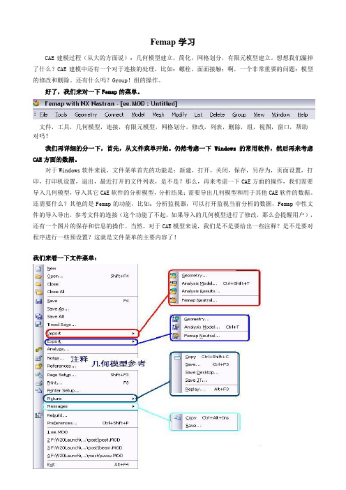
文件，工具，几何模型，连接，有限元模型，网格划分，修改，列表，删除，组，视图，窗口，帮助对吗？我们再详细的分一下，首先，从文件菜单开始。

仍然考虑一下Windows的常用软件，然后再来考虑CAE方面的数据。

对于Windows软件来说，文件菜单首先的功能是：新建，打开，关闭，保存，另存为，页面设置，打印，打印机设置，退出，最近打开的文件列表，是不是？那么，再来考虑一下CAE方面的操作，我们需要导入几何模型，导入其它CAE软件的分析模型，分析结果；需要导出几何模型和用于其他CAE软件的数据。

还需要什么？其他的是Femap的功能，比如：分析监视器，可以打开监视当前分析的数据，Femap中性文件的导入导出，参考文件的连接（这个功能了不起，如果导入的几何模型进行了修改，那么会提醒用户），还有一个图片的保存和信息的操作。

当然，对于CAE模型来说，我们是不是要给出一些注释？是不是要对程序进行一些预设置？这就是文件菜单的主要内容了！我们来看一下文件菜单：对不对？为什么有Close All呀？Femap可以同时打开多个文档，每一个文档可以有多个窗口，比如：对于一个分析模型，可以建立一个几何窗口，建立一个有限元模型的窗口，可以建立一个应力窗口，再建立一个位移窗口。

这样就需要全部关闭了！不是吗？Pcitrue里面有一个JT是什么呀？JT是UGS组织开发的3D数据交换标准。

可以用于轻量化模型，包含了几何模型的材料信息和物理属性信息，当然，可以进行剖切，打印，标注，测量，当然还可以嵌入到Office文档进行查看。

Time Save是什么呀？很简单，以前我们使用CAE程序是不是程序出错了就没有办法了，这个东西可以解决问题那么，我希望大家准备一下Femap，然后，我们来讨论一下File菜单里面的内容，关于菜单的内容就在这个主题下进行讨论吧。

调Matching前，至少准备两块板子。

一块完整PCB，有上全部零件:一块裸版，完全都没上零件:匹配前注意事项—铜管很多人忽略这点，但其实这是最重要的，因为你在调匹配过程中，会量S11(阻抗)，跟S21(Loss)。

如果铜管这边，该注意的没注意，那么你量到的S11跟S21，都是错的。

更直接一点讲，你所有的匹配工作，都是白费工。

1.铜管长度不宜过长Q. 反正我用Port Extension 把铜管校掉就好啦不对!! Port Extension不是万能的。

如果铜管过长，便无法完全校掉，如下图:由上图可知，若铜管过长，即便你做完Port Extension，其阻抗并非完美的一点Open，而是会拖一段轨迹，那么当你实际上去量PCB时，你量到的阻抗，其实包含了铜管。

也就是说，此时你量到的PCB阻抗，是不准的，是有误差的。

你若根据不准的阻抗去做匹配，你调出来的匹配永远不会好而且，不管是PCB走线，还是铜管，都一样，只要长度一长，其50奥姆就会偏掉，那就会导致Mismatch Loss。

换言之，当你实际去量PCB的Insertion Loss 时，因为包含了铜管本身的Mismatch Loss，以至于你量出来的Insertion Loss，会比PCB实际的Insertion Loss还大。

因此常有人误解，单纯量Insertion Loss，因为不看阻抗，所以不需要校正。

这是不对的观念，你量出来的阻抗错误，会连带使你量出来的Insertion Loss过大。

简单讲，只要用到铜管量S参数，不管是S11，还是S21，Open/Short/Load 校正跟Port Extension就是要做，而且铜管长度不宜过长。

2.铜管要弯折后，再做Port Extension。

因为实际上，你在做匹配时，铜管可能会弯折:如果你还没弯折时，就先做Port Extension，如下图左，即便此时你的阻抗是完美的一点Open，但是当你把铜管弯折后，其阻抗会偏，亦即此时阻抗并非完美的一点Open，如下图右:你一开始就未把铜管给校掉，亦即你量到的PCB阻抗，是不准的，是有误差的。