Matlab Exercise

实验一MATLAB介绍及其基础操作0800210402 冯晓霏1.实验目的：<1 ）熟悉MATLAB软件的集成开发环境，学习常用窗口的功能和使用方法。

<2 ）掌握帮助的使用方法以及搜索路径的添加方法。

<3 ）掌握基本的MATLAB函数操作及其使用。

<4 ）掌握简单的计算及其绘图操作。

<5 ）了解M文件的编写和运行方法。

2.实验原理<1 ）MATLAB 简介MATLAB是美国MathWorks公司开发的高性能的科学与工程计算软件。

经过几十年的扩充和完善,MATLAB已经发展成为集科学计算、可视化和编程于一体的高性能的科学计算语言和软件开发环境。

MATLAB的主要特点包括强大的矩阵计算能力、方便的绘图功能及仿真能力。

另外，MATLAB还附带了大量的专用工具箱，用于解决各种特定领域的问题。

通过学习软件的基本操作及其编程方法，体会和逐步掌握它在矩阵运算、信号处理等方面的功能及其具体应用。

通过本课程实验的学习，要求学生初步掌握MATLAB的使用方法，初步掌握M文件的编写和运行方法，初步将MATLAB运用于信号分析和系统分析中。

循序渐进地培养学生运用所学知识分析和解决问题的能力。

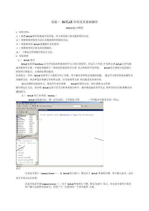
<2 ）MATLAB 的工作界面<Desktop ）MATLAB安装成功后，第一次启动时，主界面如下图< 不同版本可能有差异）所示：其中①是命令窗口<Command Window ），是MATLAB的主窗口，默认位于MATLAB 界面的右侧，用于输入命令、运行命令并显示运行结果。

②是历史命令窗<Command History ），位于MATLAB界面的左下侧，默认为前台显示。

历史命令窗用于保存用户输入过的所有的命令，为用户下一次使用同一个命令提供方便。

③是当前目录浏览器<Current Directory )，位于MATLAB界面的左上侧，默认为前台显示。

该窗口用于显示当前目录和目录中的所有文件。

MATLAB教程及实训MATLAB是一种强大的计算机软件，主要用于数值计算、数据分析和可视化，广泛应用于科学、工程和金融领域。

以下是一个针对初学者的MATLAB教程及实训，旨在帮助读者快速入门并掌握基本的MATLAB使用技巧。

第一部分：MATLAB基础1.MATLAB的安装与启动2.MATLAB命令行介绍MATLAB的命令行界面，包括如何输入和执行MATLAB命令以及查看命令的输出结果。

3.MATLAB的基本数据类型介绍MATLAB中常用的数据类型，包括标量、向量、矩阵和字符串等，并讲解如何创建和操作这些数据类型。

4.数学运算介绍如何在MATLAB中进行基本的数学运算，包括加减乘除、指数运算和三角函数等，并讲解MATLAB提供的数学函数。

5.逻辑运算和控制流程介绍如何在MATLAB中进行逻辑运算和比较运算，以及如何使用条件语句、循环语句和逻辑判断语句来控制程序的流程。

第二部分：MATLAB数据处理与分析1.数据导入和导出介绍如何使用MATLAB读取和写入各种格式的数据文件，包括文本文件、Excel文件和MAT文件等，并讲解如何处理和转换数据。

2.数据可视化介绍如何使用MATLAB绘制各种类型的图表，包括折线图、散点图、柱状图和饼图等，并讲解如何设置图表的样式和属性。

3.数据统计和分析介绍如何使用MATLAB进行常见的数据统计和分析，包括均值、方差、相关系数和回归分析等，并讲解如何使用MATLAB的统计工具箱进行高级数据分析。

第三部分：MATLAB编程与应用实例1.MATLAB编程基础介绍如何使用MATLAB编写脚本和函数，包括变量的定义和赋值、条件语句和循环语句的使用，并讲解MATLAB的函数库和程序调试技巧。

2.MATLAB的应用实例介绍几个典型的MATLAB应用实例，包括信号处理、图像处理和机器学习等领域，通过实际案例演示如何使用MATLAB解决实际问题。

3.MATLAB与其他工具的集成介绍如何将MATLAB与其他科学计算和数据处理工具集成，包括Python、R和Excel等，并讲解如何使用MATLAB的接口进行数据交互和共享。

数学实验答案Chapter 1Page20,ex1(5) 等于[exp(1),exp(2);exp(3),exp(4)](7) 3=1*3, 8=2*4(8) a为各列最小值，b为最小值所在的行号(10) 1>=4,false, 2>=3,false, 3>=2, ture, 4>=1,ture(11) 答案表明：编址第2元素满足不等式(30>=20)和编址第4元素满足不等式(40>=10)(12) 答案表明：编址第2行第1列元素满足不等式(30>=20)和编址第2行第2列元素满足不等式(40>=10)Page20, ex2(1)a, b, c的值尽管都是1，但数据类型分别为数值，字符，逻辑，注意a与c相等，但他们不等于b(2)double(fun)输出的分别是字符a,b,s,(,x,)的ASCII码Page20,ex3>> r=2;p=0.5;n=12;>> T=log(r)/n/log(1+0.01*p)Page20,ex4>> x=-2:0.05:2;f=x.^4-2.^x;>> [fmin,min_index]=min(f)最小值最小值点编址>> x(min_index)ans =0.6500 最小值点>> [f1,x1_index]=min(abs(f)) 求近似根--绝对值最小的点f1 =0.0328x1_index =24>> x(x1_index)ans =-0.8500>> x(x1_index)=[];f=x.^4-2.^x; 删去绝对值最小的点以求函数绝对值次小的点>> [f2,x2_index]=min(abs(f)) 求另一近似根--函数绝对值次小的点f2 =0.0630x2_index =65>> x(x2_index)ans =1.2500>> z=magic(10)z =92 99 1 8 15 67 74 51 58 4098 80 7 14 16 73 55 57 64 414 81 88 20 22 54 56 63 70 4785 87 19 21 3 60 62 69 71 2886 93 25 2 9 61 68 75 52 3417 24 76 83 90 42 49 26 33 6523 5 82 89 91 48 30 32 39 6679 6 13 95 97 29 31 38 45 7210 12 94 96 78 35 37 44 46 5311 18 100 77 84 36 43 50 27 59>> sum(z)>> sum(diag(z))>> z(:,2)/sqrt(3)>> z(8,:)=z(8,:)+z(3,:)Chapter 2Page 45 ex1先在编辑器窗口写下列M函数，保存为eg2_1.m function [xbar,s]=ex2_1(x)n=length(x);xbar=sum(x)/n;s=sqrt((sum(x.^2)-n*xbar^2)/(n-1));例如>>x=[81 70 65 51 76 66 90 87 61 77];>>[xbar,s]=ex2_1(x)Page 45 ex2s=log(1);n=0;while s<=100n=n+1;s=s+log(1+n);endm=nPage 40 ex3clear;F(1)=1;F(2)=1;k=2;x=0;e=1e-8; a=(1+sqrt(5))/2;while abs(x-a)>ek=k+1;F(k)=F(k-1)+F(k-2); x=F(k)/F(k-1);enda,x,k计算至k=21可满足精度clear;tic;s=0;for i=1:1000000s=s+sqrt(3)/2^i;ends,toctic;s=0;i=1;while i<=1000000s=s+sqrt(3)/2^i;i=i+1;ends,toctic;s=0;i=1:1000000;s=sqrt(3)*sum(1./2.^i);s,tocPage 45 ex5t=0:24;c=[15 14 14 14 14 15 16 18 20 22 23 25 28 ...31 32 31 29 27 25 24 22 20 18 17 16];plot(t,c)Page 45 ex6(1)x=-2:0.1:2;y=x.^2.*sin(x.^2-x-2);plot(x,y)y=inline('x^2*sin(x^2-x-2)');fplot(y,[-2 2]) (2)参数方法t=linspace(0,2*pi,100);x=2*cos(t);y=3*sin(t); plot(x,y)(3)x=-3:0.1:3;y=x;[x,y]=meshgrid(x,y);z=x.^2+y.^2;surf(x,y,z)(4)x=-3:0.1:3;y=-3:0.1:13;[x,y]=meshgrid(x,y);z=x.^4+3*x.^2+y.^2-2*x-2*y-2*x.^2.*y+6;surf(x,y,z)(5)t=0:0.01:2*pi;x=sin(t);y=cos(t);z=cos(2*t);plot3(x,y,z)(6)theta=linspace(0,2*pi,50);fai=linspace(0,pi/2,20); [theta,fai]=meshgrid(theta,fai);x=2*sin(fai).*cos(theta);y=2*sin(fai).*sin(theta);z=2*cos(fai);surf(x,y,z)(7)x=linspace(0,pi,100);y1=sin(x);y2=sin(x).*sin(10*x);y3=-sin(x);plot(x,y1,x,y2,x,y3)page45, ex7x=-1.5:0.05:1.5;y=1.1*(x>1.1)+x.*(x<=1.1).*(x>=-1.1)-1.1*(x<-1.1);plot(x,y)page45,ex9clear;close;x=-2:0.1:2;y=x;[x,y]=meshgrid(x,y);a=0.5457;b=0.7575;p=a*exp(-0.75*y.^2-3.75*x.^2-1.5*x).*(x+y>1);p=p+b*exp(-y.^2-6*x.^2).*(x+y>-1).*(x+y<=1);p=p+a*exp(-0.75*y.^2-3.75*x.^2+1.5*x).*(x+y<=-1);mesh(x,y,p)page45, ex10lookfor lyapunovhelp lyap>> A=[1 2 3;4 5 6;7 8 0];C=[2 -5 -22;-5 -24 -56;-22 -56 -16];>> X=lyap(A,C)X =1.0000 -1.0000 -0.0000-1.0000 2.0000 1.0000-0.0000 1.0000 7.0000Chapter 3Page65 Ex1>> a=[1,2,3];b=[2,4,3];a./b,a.\b,a/b,a\bans =0.5000 0.5000 1.0000ans =2 2 1ans =0.6552 一元方程组x[2,4,3]=[1,2,3]的近似解ans =0 0 00 0 00.6667 1.3333 1.0000矩阵方程[1,2,3][x11,x12,x13;x21,x22,x23;x31,x32,x33]=[2,4,3]的特解Page65 Ex 2(1)>> A=[4 1 -1;3 2 -6;1 -5 3];b=[9;-2;1];>> rank(A), rank([A,b]) [A,b]为增广矩阵ans =3ans =3 可见方程组唯一解>> x=A\bx =2.38301.48942.0213(2)>> A=[4 -3 3;3 2 -6;1 -5 3];b=[-1;-2;1];>> rank(A), rank([A,b])ans =3ans =3 可见方程组唯一解>> x=A\bx =-0.4706-0.2941(3)>> A=[4 1;3 2;1 -5];b=[1;1;1];>> rank(A), rank([A,b])ans =2ans =3 可见方程组无解>> x=A\bx =0.3311-0.1219 最小二乘近似解(4)>> a=[2,1,-1,1;1,2,1,-1;1,1,2,1];b=[1 2 3]';%注意b的写法>> rank(a),rank([a,b])ans =3ans =3 rank(a)==rank([a,b])<4说明有无穷多解>> a\bans =110 一个特解Page65 Ex3>> a=[2,1,-1,1;1,2,1,-1;1,1,2,1];b=[1,2,3]';>> x=null(a),x0=a\bx =-0.62550.6255-0.20850.4170x0 =11通解kx+x0Page65 Ex 4>> x0=[0.2 0.8]';a=[0.99 0.05;0.01 0.95];>> x1=a*x, x2=a^2*x, x10=a^10*x>> x=x0;for i=1:1000,x=a*x;end,xx =0.83330.1667>> x0=[0.8 0.2]';>> x=x0;for i=1:1000,x=a*x;end,xx =0.83330.1667>> [v,e]=eig(a)v =0.9806 -0.70710.1961 0.7071e =1.0000 00 0.9400>> v(:,1)./xans =1.17671.1767 成比例，说明x是最大特征值对应的特征向量Page65 Ex5用到公式(3.11)(3.12)>> B=[6,2,1;2.25,1,0.2;3,0.2,1.8];x=[25 5 20]'; >> C=B/diag(x)C =0.2400 0.4000 0.05000.0900 0.2000 0.01000.1200 0.0400 0.0900>> A=eye(3,3)-CA =0.7600 -0.4000 -0.0500-0.0900 0.8000 -0.0100-0.1200 -0.0400 0.9100>> D=[17 17 17]';x=A\Dx =37.569625.786224.7690Page65 Ex 6(1)>> a=[4 1 -1;3 2 -6;1 -5 3];det(a),inv(a),[v,d]=eig(a) ans =-94ans =0.2553 -0.0213 0.04260.1596 -0.1383 -0.22340.1809 -0.2234 -0.0532v =0.0185 -0.9009 -0.3066-0.7693 -0.1240 -0.7248-0.6386 -0.4158 0.6170d =-3.0527 0 00 3.6760 00 0 8.3766(2)>> a=[1 1 -1;0 2 -1;-1 2 0];det(a),inv(a),[v,d]=eig(a) ans =1ans =2.0000 -2.0000 1.00001.0000 -1.0000 1.00002.0000 -3.0000 2.0000v =-0.5773 0.5774 + 0.0000i 0.5774 - 0.0000i-0.5773 0.5774 0.5774-0.5774 0.5773 - 0.0000i 0.5773 + 0.0000id =1.0000 0 00 1.0000 + 0.0000i 00 0 1.0000 - 0.0000i(3)>> A=[5 7 6 5;7 10 8 7;6 8 10 9;5 7 9 10]A =5 76 57 10 8 76 8 10 95 7 9 10>> det(A),inv(A), [v,d]=eig(A)ans =1ans =68.0000 -41.0000 -17.0000 10.0000-41.0000 25.0000 10.0000 -6.0000-17.0000 10.0000 5.0000 -3.000010.0000 -6.0000 -3.0000 2.0000v =0.8304 0.0933 0.3963 0.3803-0.5016 -0.3017 0.6149 0.5286-0.2086 0.7603 -0.2716 0.55200.1237 -0.5676 -0.6254 0.5209d =0.0102 0 0 00 0.8431 0 00 0 3.8581 00 0 0 30.2887(4)(以n=5为例)方法一（三个for）n=5;for i=1:n, a(i,i)=5;endfor i=1:(n-1),a(i,i+1)=6;endfor i=1:(n-1),a(i+1,i)=1;enda方法二（一个for）n=5;a=zeros(n,n);a(1,1:2)=[5 6];for i=2:(n-1),a(i,[i-1,i,i+1])=[1 5 6];enda(n,[n-1 n])=[1 5];a方法三（不用for）n=5;a=diag(5*ones(n,1));b=diag(6*ones(n-1,1));c=diag(ones(n-1,1));a=a+[zeros(n-1,1),b;zeros(1,n)]+[zeros(1,n);c,zeros(n-1,1)] 下列计算>> det(a)ans =665>> inv(a)ans =0.3173 -0.5865 1.0286 -1.6241 1.9489-0.0977 0.4887 -0.8571 1.3534 -1.62410.0286 -0.1429 0.5429 -0.8571 1.0286-0.0075 0.0376 -0.1429 0.4887 -0.58650.0015 -0.0075 0.0286 -0.0977 0.3173>> [v,d]=eig(a)v =-0.7843 -0.7843 -0.9237 0.9860 -0.92370.5546 -0.5546 -0.3771 -0.0000 0.3771-0.2614 -0.2614 0.0000 -0.1643 0.00000.0924 -0.0924 0.0628 -0.0000 -0.0628-0.0218 -0.0218 0.0257 0.0274 0.0257d =0.7574 0 0 0 00 9.2426 0 0 00 0 7.4495 0 00 0 0 5.0000 00 0 0 0 2.5505Page65 Ex 7(1)>> a=[4 1 -1;3 2 -6;1 -5 3];[v,d]=eig(a)v =0.0185 -0.9009 -0.3066-0.7693 -0.1240 -0.7248-0.6386 -0.4158 0.6170d =-3.0527 0 00 3.6760 00 0 8.3766>> det(v)ans =-0.9255 %v行列式正常, 特征向量线性相关，可对角化>> inv(v)*a*v 验算ans =-3.0527 0.0000 -0.00000.0000 3.6760 -0.0000-0.0000 -0.0000 8.3766>> [v2,d2]=jordan(a) 也可用jordanv2 =0.0798 0.0076 0.91270.1886 -0.3141 0.1256-0.1605 -0.2607 0.4213 特征向量不同d2 =8.3766 0 00 -3.0527 - 0.0000i 00 0 3.6760 + 0.0000i>> v2\a*v2ans =8.3766 0 0.00000.0000 -3.0527 0.00000.0000 0.0000 3.6760>> v(:,1)./v2(:,2) 对应相同特征值的特征向量成比例ans =2.44912.44912.4491(2)>> a=[1 1 -1;0 2 -1;-1 2 0];[v,d]=eig(a)v =-0.5773 0.5774 + 0.0000i 0.5774 - 0.0000i-0.5773 0.5774 0.5774-0.5774 0.5773 - 0.0000i 0.5773 + 0.0000id =1.0000 0 00 1.0000 + 0.0000i 00 0 1.0000 - 0.0000i>> det(v)ans =-5.0566e-028 -5.1918e-017i v的行列式接近0, 特征向量线性相关，不可对角化>> [v,d]=jordan(a)v =1 0 11 0 01 -1 0d =1 1 00 1 10 0 1 jordan标准形不是对角的，所以不可对角化(3)>> A=[5 7 6 5;7 10 8 7;6 8 10 9;5 7 9 10]A =5 76 57 10 8 76 8 10 95 7 9 10>> [v,d]=eig(A)v =0.8304 0.0933 0.3963 0.3803-0.5016 -0.3017 0.6149 0.5286-0.2086 0.7603 -0.2716 0.55200.1237 -0.5676 -0.6254 0.5209d =0.0102 0 0 00 0.8431 0 00 0 3.8581 00 0 0 30.2887>> inv(v)*A*vans =0.0102 0.0000 -0.0000 0.00000.0000 0.8431 -0.0000 -0.0000-0.0000 0.0000 3.8581 -0.0000-0.0000 -0.0000 0 30.2887本题用jordan不行, 原因未知(4)参考6(4)和7(1)Page65 Exercise 8只有(3)对称, 且特征值全部大于零, 所以是正定矩阵. Page65 Exercise 9(1)>> a=[4 -3 1 3;2 -1 3 5;1 -1 -1 -1;3 -2 3 4;7 -6 -7 0]>> rank(a)ans =3>> rank(a(1:3,:))ans =2>> rank(a([1 2 4],:)) 1,2,4行为最大无关组ans =3>> b=a([1 2 4],:)';c=a([3 5],:)';>> b\c 线性表示的系数ans =0.5000 5.0000-0.5000 1.00000 -5.0000Page65 Exercise 10>> a=[1 -2 2;-2 -2 4;2 4 -2]>> [v,d]=eig(a)v =0.3333 0.9339 -0.12930.6667 -0.3304 -0.6681-0.6667 0.1365 -0.7327d =-7.0000 0 00 2.0000 00 0 2.0000>> v'*vans =1.0000 0.0000 0.00000.0000 1.0000 00.0000 0 1.0000 v确实是正交矩阵Page65 Exercise 11设经过6个电阻的电流分别为i1, ..., i6. 列方程组如下20-2i1=a; 5-3i2=c; a-3i3=c; a-4i4=b; c-5i5=b; b-3i6=0;i1=i3+i4;i5=i2+i3;i6=i4+i5;计算如下>> A=[1 0 0 2 0 0 0 0 0;0 0 1 0 3 0 0 0 0;1 0 -1 0 0 -3 0 0 0; 1 -1 0 0 0 0 -4 0 0;0 -1 1 0 0 0 0 -5 0;0 1 0 0 0 0 0 0 -3; 0 0 0 1 0 -1 -1 0 0;0 0 0 0 -1 -1 0 1 0;0 0 0 0 0 0 -1 -1 1];>>b=[20 5 0 0 0 0 0 0 0]'; A\bans =13.34536.44018.54203.3274-1.18071.60111.72630.42042.1467Page65 Exercise 12>> A=[1 2 3;4 5 6;7 8 0];>> left=sum(eig(A)), right=sum(trace(A))left =6.0000right =6>> left=prod(eig(A)), right=det(A) 原题有错, (-1)^n应删去left =27.0000right =27>> fA=(A-p(1)*eye(3,3))*(A-p(2)*eye(3,3))*(A-p(3)*eye(3,3)) fA =1.0e-012 *0.0853 0.1421 0.02840.1421 0.1421 0-0.0568 -0.1137 0.1705>> norm(fA) f(A)范数接近0ans =2.9536e-013Chapter 4Page84 Exercise 1(1)roots([1 1 1])(2)roots([3 0 -4 0 2 -1])(3)p=zeros(1,24);p([1 17 18 22])=[5 -6 8 -5];roots(p)(4)p1=[2 3];p2=conv(p1, p1);p3=conv(p1, p2);p3(end)=p3(end)-4; %原p3最后一个分量-4roots(p3)Page84 Exercise 2fun=inline('x*log(sqrt(x^2-1)+x)-sqrt(x^2-1)-0.5*x');fzero(fun,2)Page84 Exercise 3fun=inline('x^4-2^x');fplot(fun,[-2 2]);grid on;fzero(fun,-1),fzero(fun,1),fminbnd(fun,0.5,1.5)Page84 Exercise 4fun=inline('x*sin(1/x)','x');fplot(fun, [-0.1 0.1]);x=zeros(1,10);for i=1:10, x(i)=fzero(fun,(i-0.5)*0.01);end;x=[x,-x]Page84 Exercise 5fun=inline('[9*x(1)^2+36*x(2)^2+4*x(3)^2-36;x(1)^2-2*x(2)^2-20*x(3);16*x(1)-x(1)^3-2*x(2)^ 2-16*x(3)^2]','x');[a,b,c]=fsolve(fun,[0 0 0])Page84 Exercise 6fun=@(x)[x(1)-0.7*sin(x(1))-0.2*cos(x(2)),x(2)-0.7*cos(x(1))+0.2*sin(x(2))];[a,b,c]=fsolve(fun,[0.5 0.5])Page84 Exercise 7clear; close; t=0:pi/100:2*pi;x1=2+sqrt(5)*cos(t); y1=3-2*x1+sqrt(5)*sin(t);x2=3+sqrt(2)*cos(t); y2=6*sin(t);plot(x1,y1,x2,y2); grid on; 作图发现4个解的大致位置，然后分别求解y1=fsolve('[(x(1)-2)^2+(x(2)-3+2*x(1))^2-5,2*(x(1)-3)^2+(x(2)/3)^2-4]',[1.5,2])y2=fsolve('[(x(1)-2)^2+(x(2)-3+2*x(1))^2-5,2*(x(1)-3)^2+(x(2)/3)^2-4]',[1.8,-2])y3=fsolve('[(x(1)-2)^2+(x(2)-3+2*x(1))^2-5,2*(x(1)-3)^2+(x(2)/3)^2-4]',[3.5,-5])y4=fsolve('[(x(1)-2)^2+(x(2)-3+2*x(1))^2-5,2*(x(1)-3)^2+(x(2)/3)^2-4]',[4,-4])Page84 Exercise 8(1)clear;fun=inline('x.^2.*sin(x.^2-x-2)');fplot(fun,[-2 2]);grid on; 作图观察x(1)=-2;x(3)=fminbnd(fun,-1,-0.5);x(5)=fminbnd(fun,1,2);fun2=inline('-x.^2.*sin(x.^2-x-2)');x(2)=fminbnd(fun2,-2,-1);x(4)=fminbnd(fun2,-0.5,0.5);x(6)=2feval(fun,x)答案: 以上x(1)(3)(5)是局部极小，x(2)(4)(6)是局部极大，从最后一句知道x(1)全局最小，x(2)最大。

matlab函数大全Matlab函数大全。

Matlab是一种强大的数学软件，它提供了丰富的函数库，可以帮助用户进行各种数学计算、数据分析和可视化操作。

在Matlab中，函数是一种用来完成特定任务的代码块，它可以接受输入参数并返回输出结果。

本文将介绍一些常用的Matlab函数，希望能够帮助读者更好地理解和使用Matlab。

1. plot函数。

plot函数是Matlab中最常用的函数之一，它用于绘制二维图形。

通过plot函数，用户可以将数据点连接起来，形成折线图或者曲线图。

plot函数的基本语法是，plot(x, y)，其中x和y分别表示横轴和纵轴的数据点。

用户可以通过设置不同的参数，如颜色、线型、线宽等，来定制绘制的图形。

2. linspace函数。

linspace函数用于生成指定范围内的等间距数据点。

其基本语法是，linspace(start, end, n)，其中start和end分别表示起始值和终止值，n表示生成的数据点个数。

linspace函数常用于生成绘图的横轴数据点，也可以用于生成一维数组。

3. meshgrid函数。

meshgrid函数用于生成二维网格数据点。

其基本语法是，[X, Y] = meshgrid(x, y)，其中x和y分别表示横轴和纵轴的数据点，X和Y分别表示生成的二维网格数据点。

meshgrid函数常用于三维曲面的绘制，也可以用于生成二维数组。

4. fft函数。

fft函数用于进行快速傅里叶变换，它可以将时域信号转换为频域信号。

其基本语法是，Y = fft(X)，其中X表示输入的时域信号，Y表示输出的频域信号。

fft函数常用于信号处理和频谱分析。

5. polyfit函数。

polyfit函数用于进行多项式拟合，它可以根据给定的数据点拟合出一个多项式模型。

其基本语法是，p = polyfit(x, y, n)，其中x和y表示数据点，n表示拟合的多项式阶数，p表示拟合出的多项式系数。

MATLAB 程序设计及应用习题二维平面绘图1． 椭圆的参数表示为⎩⎨⎧==)sin()cos(t b y t a x ，请利用这个公式画一个椭圆，其中a=5,b=3要求椭圆上有100个点。

2． Chebysheve 多项式的定义如下：11)),(cos cos(1≤≤-=-x x m y ;当m 的值从1变化到5时，得到五条曲线。

请将这五条曲线画在同一张图上。

使用legend 命令来标记每一条曲线。

3． 用contour 命令画出下列隐函数：2522=+y x 。

提示：画出函数：22y x z +=高度为25的等高线。

三维立体绘图1． 请利用surf 命令画出函数：)ex p(*22y x x z --=的图形。

其中x 在[-2，2]范围内均匀取21个点，y 在[-1，1]范围内均匀取21个点。

2． 一个空间的椭球可以表示为1222222=++cz b y a x ，请使用任何方法画出一个空间的光滑的椭球。

其中a=3,b=4,c=8。

3． 画出函数)cos()2/sin(),(y x y x f =的曲面图和等高线图，其中x 在[-2π，2π]范围内均匀取21个点，y 在[-1.5π，1.5π]范围内均匀取31个点。

用subplot(2,1,1)和subplot(2,1,2)将的曲面图和等高线图画在一个窗口中。

特殊图形1． 以下是某学校信息系各年度的人员组成表，请分别用bar 和bar3画出上述数据的统计图。

2． 请使用上题的数据作出（1）按每年度人数来划分的立体扇形图，并加上适当的说明。

（2）按每种类别人数来划分的立体扇形图，并加上适当的说明。

图象的显示与读写1．读入文件clown.mat中的小丑图象，显示图象，并将调色板colormap改为grey,你会发现图象偏暗，请调整调色板，使其亮度提高。

2．读入文件clown.mat中的小丑图象，显示图象，请调整调色板，使得显示的图象由全黑或全白的象素做成，且其个数的比例大约是1:1。

MATLAB命令汇总1.基本运算：-`+`:加法运算-`-`:减法运算-`*`:乘法运算-`/`:除法运算-`^`或`**`:幂运算- `sqrt(`: 平方根函数- `exp(`: 指数函数- `log(`: 对数函数2.矩阵和向量：- `zeros(`: 创建全零矩阵- `ones(`: 创建全一矩阵- `eye(`: 创建单位矩阵- `rand(`: 创建随机矩阵- `diag(`: 提取矩阵的对角线元素- `transpose(`或`'`: 转置矩阵- `det(`: 求矩阵的行列式- `inv(`: 求矩阵的逆矩阵- `trace(`: 求矩阵的迹3.数据处理和统计函数：- `mean(`: 求平均值- `median(`: 求中位数- `std(`: 求标准差- `var(`: 求方差- `sort(`: 排序- `histogram(`: 绘制直方图- `corrcoef(`: 计算相关系数矩阵- `cov(`: 计算协方差矩阵- `unique(`: 去掉重复元素4.数据可视化：- `plot(`: 绘制二维折线图- `scatter(`: 绘制散点图- `bar(`: 绘制柱状图- `hist(`: 绘制直方图- `pie(`: 绘制饼图- `imagesc(`: 绘制热图- `contour(`: 绘制等高线图- `surf(`: 绘制三维曲面图5.逻辑和条件语句：- `if`: 条件判断语句- `else`: 条件判断的可选分支- `elseif`: 多个条件判断的中间分支- `while`: 循环语句- `for`: 循环语句- `break`: 跳出循环- `continue`: 跳过本次循环6.文件和数据输入输出：- `load(`: 从文件加载数据- `save(`: 将数据保存到文件- `fopen(`: 打开文件- `fclose(`: 关闭文件- `fprintf(`: 格式化输出到文件- `fscanf(`: 从文件按格式读取数据7.函数和脚本文件：- `function`: 定义函数- `script`: 脚本文件- `input(`: 从命令行输入数据- `disp(`: 显示结果或变量值- `return`: 返回函数结果- `clear(`: 清除变量或内存- `clc(`: 清除命令窗口内容以上是一些常用的MATLAB命令和函数的汇总，这只是冰山一角，MATLAB还提供了许多其他功能和扩展性更强的函数和工具箱，可以根据不同的需求进行更详细的学习和使用。

信号与系统实验报告实验一、信号基本运算的MATLAB 实现一、实验目的学习如何利用Matlab 实现信号的基本运算，掌握信号的基本运算的原理，加深对书本知识的理解。

二、实验材料PC 机一台三、实验内容1、（1）编写如图Exercise1.1所示波形的MATLAB 函数。

（2）试画出f(t),f(0.5t),f(1-2t)的波形。

解：程序如下： 实验结果： function yt = f2(t)yt=tripuls(t,4,0.5); t=-3:0.01:5; subplot(311) plot(t,tx(t)) title('f£¨t£©') subplot(312) plot(t,tx(0.5*t)) title('f(0.5t)') subplot(313) plot(t,tx(-2*t)) title('f(-2t)') 2、画出如图exercise1.2所示序列f[2k]、f[-k]和f[k+2],f[k-2]的波形。

并求f[k]的和。

解：程序如下：function f=ls(k)f=3.*(k==-2)+1.*(k==-1)+(-2).*(k==0)+(-1).*(k==1)+2.*(k==2)+(-3).*(k==3);Exercise 1.1－3f[k] kExercise1.2k=-5:0.01:10;subplot(321)stem(k,ls(k)) 实验结果：title('f[k]')subplot(322)stem(k,ls(2*k))title('f[2k]')subplot(323)stem(k,ls(-1*k))title('f[-k]')subplot(324)stem(k,ls(k+2))title('f[k+2]')subplot(325)stem(k,ls(k-2))title('f[k-2]')subplot(326)plot(k,sum(ls(-2:3)))title('Sum f[k]')3、解：程序如下：function y=tx(t)y=0.*(t>=2|t<-1)+(2-t).*(t>=1&t<2)+1.*(t>=-1&t<1); t=-5:0.01:5; 实验结果：ft1=tripuls(t-3,2,0.5);subplot(311)plot(t,ft1)title('f(t)')ft1=tripuls(-t-3,2,0.5);subplot(312)plot(t,ft1)title('f(-t)')ft1=tripuls(-2*t-2,2,0.5);subplot(313)plot(t,ft1)title('f(1-2t)')。

数学实验MATLAB参考答案（重要部分）P20,ex1(5) 等于[exp(1),exp(2);exp(3),exp(4)](7) 3=1*3, 8=2*4(8) a为各列最小值，b为最小值所在的行号(10) 1>=4,false, 2>=3,false, 3>=2, ture, 4>=1,ture(11) 答案表明：编址第2元素满足不等式(30>=20)和编址第4元素满足不等式(40>=10)(12) 答案表明：编址第2行第1列元素满足不等式(30>=20)和编址第2行第2列元素满足不等式(40>=10)P20, ex2(1)a, b, c的值尽管都是1，但数据类型分别为数值，字符，逻辑，注意a 与c相等，但他们不等于b(2)double(fun)输出的分别是字符a,b,s,(,x,)的ASCII码P20,ex3>> r=2;p=0.5;n=12;>> T=log(r)/n/log(1+0.01*p)T =11.5813P20,ex4>> x=-2:0.05:2;f=x.^4-2.^x;>> [fmin,min_index]=min(f)fmin =-1.3907 %最小值min_index =54 %最小值点编址>> x(min_index)ans =0.6500 %最小值点>> [f1,x1_index]=min(abs(f)) %求近似根--绝对值最小的点f1 =0.0328x1_index =24>> x(x1_index)ans =-0.8500>> x(x1_index)=[];f=x.^4-2.^x; %删去绝对值最小的点以求函数绝对值次小的点>> [f2,x2_index]=min(abs(f)) %求另一近似根--函数绝对值次小的点f2 =0.0630x2_index =65>> x(x2_index)ans =1.2500P20,ex5>> z=magic(10)z =92 99 1 8 15 67 74 51 58 4098 80 7 14 16 73 55 57 64 414 81 88 20 22 54 56 63 70 4785 87 19 21 3 60 62 69 71 2886 93 25 2 9 61 68 75 52 3417 24 76 83 90 42 49 26 33 6579 6 13 95 97 29 31 38 45 7210 12 94 96 78 35 37 44 46 5311 18 100 77 84 36 43 50 27 59>> sum(z)ans =505 505 505 505 505 505 505 505 505 505 >> sum(diag(z))ans =505>> z(:,2)/sqrt(3)ans =57.157746.188046.765450.229553.693613.85642.88683.46416.928210.3923>> z(8,:)=z(8,:)+z(3,:)z =92 99 1 8 15 67 74 51 58 4098 80 7 14 16 73 55 57 64 414 81 88 20 22 54 56 63 70 4785 87 19 21 3 60 62 69 71 2886 93 25 2 9 61 68 75 52 3423 5 82 89 91 48 30 32 39 6683 87 101 115 119 83 87 101 115 11910 12 94 96 78 35 37 44 46 5311 18 100 77 84 36 43 50 27 59P 40 ex1先在编辑器窗口写下列M函数，保存为eg2_1.m function [xbar,s]=ex2_1(x)n=length(x);xbar=sum(x)/n;s=sqrt((sum(x.^2)-n*xbar^2)/(n-1));例如>>x=[81 70 65 51 76 66 90 87 61 77];>>[xbar,s]=ex2_1(x)xbar =72.4000s =12.1124P 40 ex2s=log(1);n=0;while s<=100n=n+1;s=s+log(1+n);endm=n计算结果m=37clear;F(1)=1;F(2)=1;k=2;x=0;e=1e-8; a=(1+sqrt(5))/2;while abs(x-a)>ek=k+1;F(k)=F(k-1)+F(k-2); x=F(k)/F(k-1); enda,x,k计算至k=21可满足精度P 40 ex4clear;tic;s=0;for i=1:1000000s=s+sqrt(3)/2^i;ends,toctic;s=0;i=1;while i<=1000000s=s+sqrt(3)/2^i;i=i+1;ends,toctic;s=0;i=1:1000000;s=sqrt(3)*sum(1./2.^i);s,tocP 40 ex5c=[15 14 14 14 14 15 16 18 20 22 23 25 28 ...31 32 31 29 27 25 24 22 20 18 17 16];plot(t,c)P 40 ex6(1)clear;fplot('x^2*sin(x^2-x-2)',[-2,2])x=-2:0.1:2;y=x.^2.*sin(x.^2-x-2);plot(x,y)y=inline('x^2*sin(x^2-x-2)');fplot(y,[-2 2])(2)参数方法t=linspace(0,2*pi,100);x=2*cos(t);y=3*sin(t); plot(x,y)(3)x=-3:0.1:3;y=x;[x,y]=meshgrid(x,y);z=x.^2+y.^2;surf(x,y,z)(4)x=-3:0.1:3;y=-3:0.1:13;[x,y]=meshgrid(x,y);z=x.^4+3*x.^2+y.^2-2*x-2*y-2*x.^2.*y+6;surf(x,y,z)(5)t=0:0.01:2*pi;x=sin(t);y=cos(t);z=cos(2*t);plot3(x,y,z)(6)theta=linspace(0,2*pi,50);fai=linspace(0,pi/2,20);[theta,fai]=meshgrid(theta,fai); x=2*sin(fai).*cos(theta);y=2*sin(fai).*sin(theta);z=2*cos(fai);surf(x,y,z)(7)x=linspace(0,pi,100);y1=sin(x);y2=sin(x).*sin(10*x);y3=-sin(x);plot(x,y1,x,y2,x,y3)page41, ex7x=-1.5:0.05:1.5;y=1.1*(x>1.1)+x.*(x<=1.1).*(x>=-1.1)-1.1*(x<-1.1);plot(x,y)page41,ex8分别使用which trapz, type trapz, dir C:\MATLAB7\toolbox\matlab\datafun\ page41,ex9clear;close;x=-2:0.1:2;y=x;[x,y]=meshgrid(x,y);a=0.5457;b=0.7575;p=a*exp(-0.75*y.^2-3.75*x.^2-1.5*x).*(x+y>1);p=p+b*exp(-y.^2-6*x.^2).*(x+y>-1).*(x+y<=1);p=p+a*exp(-0.75*y.^2-3.75*x.^2+1.5*x).*(x+y<=-1);mesh(x,y,p)page41, ex10lookfor lyapunovhelp lyap>> A=[1 2 3;4 5 6;7 8 0];C=[2 -5 -22;-5 -24 -56;-22 -56 -16];>> X=lyap(A,C)X =1.0000 -1.0000 -0.0000 -1.00002.0000 1.0000 -0.0000 1.0000 7.0000Chapter 3%Exercise 1>> a=[1,2,3];b=[2,4,3];a./b,a.\b,a/b,a\bans =0.5000 0.5000 1.0000ans =2 2 1ans =0.6552 %一元方程组x[2,4,3]=[1,2,3]的近似解ans =0 0 00 0 00.6667 1.3333 1.0000%矩阵方程[1,2,3][x11,x12,x13;x21,x22,x23;x31,x32,x33]=[2,4,3]的特解Exercise 2(1)>> A=[4 1 -1;3 2 -6;1 -5 3];b=[9;-2;1];>> rank(A), rank([A,b]) %[A,b]为增广矩阵ans =3ans =3 %可见方程组唯一解>> x=A\bx =2.38301.48942.0213Exercise 2(2)>> A=[4 -3 3;3 2 -6;1 -5 3];b=[-1;-2;1];>> rank(A), rank([A,b]) ans =3ans =3 %可见方程组唯一解>> x=A\bx =-0.4706-0.2941Exercise 2(3)>> A=[4 1;3 2;1 -5];b=[1;1;1];>> rank(A), rank([A,b])ans =2ans =3 %可见方程组无解>> x=A\bx =0.3311-0.1219 %最小二乘近似解Exercise 2(4)>> a=[2,1,-1,1;1,2,1,-1;1,1,2,1];b=[1 2 3]';%注意b的写法>> rank(a),rank([a,b])ans =3ans =3 %rank(a)==rank([a,b])<4说明有无穷多解>> a\bans =110 %一个特解Exercise 3>> a=[2,1,-1,1;1,2,1,-1;1,1,2,1];b=[1,2,3]';>> x=null(a),x0=a\bx =-0.62550.6255-0.20850.4170x0 =11%通解kx+x0 Exercise 4>> x0=[0.2 0.8]';a=[0.99 0.05;0.01 0.95];>> x1=a*x, x2=a^2*x, x10=a^10*x>> x=x0;for i=1:1000,x=a*x;end,xx =0.83330.1667>> x0=[0.8 0.2]';>> x=x0;for i=1:1000,x=a*x;end,xx =0.83330.1667>> [v,e]=eig(a)v =0.9806 -0.70710.1961 0.7071e =1.0000 00 0.9400>> v(:,1)./xans =1.17671.1767 %成比例，说明x是最大特征值对应的特征向量Exercise 5%用到公式(3.11)(3.12)>> B=[6,2,1;2.25,1,0.2;3,0.2,1.8];x=[25 5 20]'; >> C=B/diag(x)C =0.2400 0.4000 0.05000.0900 0.2000 0.0100 0.1200 0.0400 0.0900 >> A=eye(3,3)-CA =0.7600 -0.4000 -0.0500 -0.0900 0.8000 -0.0100 -0.1200 -0.0400 0.9100 >> D=[17 17 17]';x=A\D x =37.569625.786224.7690%Exercise 6(1)>> a=[4 1 -1;3 2 -6;1 -5 3];det(a),inv(a),[v,d]=eig(a) ans =-94ans =0.2553 -0.0213 0.04260.1596 -0.1383 -0.22340.1809 -0.2234 -0.0532v =0.0185 -0.9009 -0.3066-0.7693 -0.1240 -0.7248-0.6386 -0.4158 0.6170d =-3.0527 0 00 3.6760 00 0 8.3766%Exercise 6(2)>> a=[1 1 -1;0 2 -1;-1 2 0];det(a),inv(a),[v,d]=eig(a) ans =1ans =2.0000 -2.0000 1.00001.0000 -1.0000 1.00002.0000 -3.0000 2.0000v =-0.5773 0.5774 + 0.0000i 0.5774 - 0.0000i-0.5773 0.5774 0.5774-0.5774 0.5773 - 0.0000i 0.5773 + 0.0000id =1.0000 0 00 1.0000 + 0.0000i 00 0 1.0000 - 0.0000i%Exercise 6(3)>> A=[5 7 6 5;7 10 8 7;6 8 10 9;5 7 9 10]A =5 76 57 10 8 76 8 10 95 7 9 10>> det(A),inv(A), [v,d]=eig(A)ans =1ans =68.0000 -41.0000 -17.0000 10.0000-41.0000 25.0000 10.0000 -6.0000-17.0000 10.0000 5.0000 -3.000010.0000 -6.0000 -3.0000 2.0000v =0.8304 0.0933 0.3963 0.3803-0.5016 -0.3017 0.6149 0.5286-0.2086 0.7603 -0.2716 0.55200.1237 -0.5676 -0.6254 0.5209d =0.0102 0 0 00 0.8431 0 00 0 3.8581 00 0 0 30.2887%Exercise 6(4)、(以n=5为例)%关键是矩阵的定义%方法一（三个for）n=5;for i=1:n, a(i,i)=5;endfor i=1:(n-1),a(i,i+1)=6;endfor i=1:(n-1),a(i+1,i)=1;enda%方法二（一个for）n=5;a=zeros(n,n);a(1,1:2)=[5 6];for i=2:(n-1),a(i,[i-1,i,i+1])=[1 5 6];enda(n,[n-1 n])=[1 5];a%方法三（不用for）n=5;a=diag(5*ones(n,1));b=diag(6*ones(n-1,1));c=diag(ones(n-1,1));a=a+[zeros(n-1,1),b;zeros(1,n)]+[zeros(1,n);c,zeros(n-1,1)] %下列计算>> det(a)ans =665>> inv(a)ans =0.3173 -0.5865 1.0286 -1.6241 1.9489-0.0977 0.4887 -0.8571 1.3534 -1.62410.0286 -0.1429 0.5429 -0.8571 1.0286-0.0075 0.0376 -0.1429 0.4887 -0.5865 0.0015 -0.0075 0.0286 -0.0977 0.3173 >> [v,d]=eig(a)v =-0.7843 -0.7843 -0.9237 0.9860 -0.9237 0.5546 -0.5546 -0.3771 -0.0000 0.3771-0.2614 -0.2614 0.0000 -0.1643 0.0000 0.0924 -0.0924 0.0628 -0.0000 -0.0628-0.0218 -0.0218 0.0257 0.0274 0.0257d =0.7574 0 0 0 00 9.2426 0 0 00 0 7.4495 0 00 0 0 5.0000 00 0 0 0 2.5505%Exercise 7(1)>> a=[4 1 -1;3 2 -6;1 -5 3];[v,d]=eig(a) v =0.0185 -0.9009 -0.3066-0.7693 -0.1240 -0.7248-0.6386 -0.4158 0.6170d =-3.0527 0 00 3.6760 00 0 8.3766>> det(v)ans =-0.9255 %v行列式正常, 特征向量线性相关，可对角化>> inv(v)*a*v %验算ans =-3.0527 0.0000 -0.00000.0000 3.6760 -0.0000-0.0000 -0.0000 8.3766>> [v2,d2]=jordan(a) %也可用jordanv2 =0.0798 0.0076 0.91270.1886 -0.3141 0.1256-0.1605 -0.2607 0.4213 %特征向量不同d2 =8.3766 0 00 -3.0527 - 0.0000i 00 0 3.6760 + 0.0000i>> v2\a*v2ans =8.3766 0 0.00000.0000 -3.0527 0.00000.0000 0.0000 3.6760>> v(:,1)./v2(:,2) %对应相同特征值的特征向量成比例ans =2.44912.44912.4491%Exercise 7(2)>> a=[1 1 -1;0 2 -1;-1 2 0];[v,d]=eig(a)v =-0.5773 0.5774 + 0.0000i 0.5774 - 0.0000i-0.5773 0.5774 0.5774-0.5774 0.5773 - 0.0000i 0.5773 + 0.0000id =1.0000 0 00 1.0000 + 0.0000i 00 0 1.0000 - 0.0000i>> det(v)ans =-5.0566e-028 -5.1918e-017i %v的行列式接近0, 特征向量线性相关，不可对角化>> [v,d]=jordan(a)v =1 0 11 -1 0d =1 1 00 1 10 0 1 %jordan标准形不是对角的，所以不可对角化%Exercise 7(3)>> A=[5 7 6 5;7 10 8 7;6 8 10 9;5 7 9 10]A =5 76 57 10 8 76 8 10 95 7 9 10>> [v,d]=eig(A)0.8304 0.0933 0.3963 0.3803-0.5016 -0.3017 0.6149 0.5286-0.2086 0.7603 -0.2716 0.55200.1237 -0.5676 -0.6254 0.5209d =0.0102 0 0 00 0.8431 0 00 0 3.8581 00 0 0 30.2887>> inv(v)*A*vans =0.0102 0.0000 -0.0000 0.00000.0000 0.8431 -0.0000 -0.0000-0.0000 0.0000 3.8581 -0.0000-0.0000 -0.0000 0 30.2887%本题用jordan不行, 原因未知%Exercise 7(4)参考6(4)和7(1), 略%Exercise 8 只有(3)对称, 且特征值全部大于零, 所以是正定矩阵. %Exercise 9(1)>> a=[4 -3 1 3;2 -1 3 5;1 -1 -1 -1;3 -2 3 4;7 -6 -7 0]>> rank(a)ans =3>> rank(a(1:3,:))ans =2>> rank(a([1 2 4],:)) %1,2,4行为最大无关组3>> b=a([1 2 4],:)';c=a([3 5],:)'; >> b\c %线性表示的系数ans =0.5000 5.0000-0.5000 1.00000 -5.0000%Exercise 10>> a=[1 -2 2;-2 -2 4;2 4 -2]>> [v,d]=eig(a)0.3333 0.9339 -0.12930.6667 -0.3304 -0.6681-0.6667 0.1365 -0.7327d =-7.0000 0 00 2.0000 00 0 2.0000>> v'*vans =1.0000 0.0000 0.00000.0000 1.0000 00.0000 0 1.0000 %v确实是正交矩阵%Exercise 11%设经过6个电阻的电流分别为i1, ..., i6. 列方程组如下%20-2i1=a; 5-3i2=c; a-3i3=c; a-4i4=b; c-5i5=b; b-3i6=0; %i1=i3+i4;i5=i2+i3;i6=i4+i5;%计算如下>> A=[1 0 0 2 0 0 0 0 0;0 0 1 0 3 0 0 0 0;1 0 -1 0 0 -3 0 0 0;1 -1 0 0 0 0 -4 0 0;0 -1 1 0 0 0 0 -5 0;0 1 0 0 0 0 0 0 -3;0 0 0 1 0 -1 -1 0 0;0 0 0 0 -1 -1 0 1 0;0 0 0 0 0 0 -1 -1 1];>>b=[20 5 0 0 0 0 0 0 0]'; A\bans =13.34536.44018.54203.3274-1.18071.60111.72630.42042.1467%Exercise 12>> A=[1 2 3;4 5 6;7 8 0];>> left=sum(eig(A)), right=sum(trace(A))left =6.0000right =6>> left=prod(eig(A)), right=det(A) %原题有错, (-1)^n应删去left =27.0000right =27>> fA=(A-p(1)*eye(3,3))*(A-p(2)*eye(3,3))*(A-p(3)*eye(3,3))fA =1.0e-012 *0.0853 0.1421 0.02840.1421 0.1421 0-0.0568 -0.1137 0.1705>> norm(fA) %f(A)范数接近0ans =2.9536e-013%Exercise 1(1)roots([1 1 1])%Exercise 1(2)roots([3 0 -4 0 2 -1])%Exercise 1(3)p=zeros(1,24);p([1 17 18 22])=[5 -6 8 -5];roots(p)%Exercise 1(4)p1=[2 3];p2=conv(p1, p1);p3=conv(p1, p2);p3(end)=p3(end)-4; %原p3最后一个分量-4roots(p3)%Exercise 2fun=inline('x*log(sqrt(x^2-1)+x)-sqrt(x^2-1)-0.5*x'); fzero(fun,2)】%Exercise 3fun=inline('x^4-2^x');fplot(fun,[-2 2]);grid on;fzero(fun,-1),fzero(fun,1),fminbnd(fun,0.5,1.5)%Exercise 4fun=inline('x*sin(1/x)','x');fplot(fun, [-0.1 0.1]);x=zeros(1,10);for i=1:10, x(i)=fzero(fun,(i-0.5)*0.01);end;x=[x,-x]%Exercise 5fun=inline('[9*x(1)^2+36*x(2)^2+4*x(3)^2-36;x(1)^2-2*x(2)^2-20*x(3);16*x(1)-x(1)^3-2*x(2)^2-16*x(3)^2]','x');[a,b,c]=fsolve(fun,[0 0 0])%Exercise 6fun=@(x)[x(1)-0.7*sin(x(1))-0.2*cos(x(2)),x(2)-0.7*cos(x(1))+0.2*sin(x(2))];[a,b,c]=fsolve(fun,[0.5 0.5])%Exercise 7clear; close; t=0:pi/100:2*pi; x1=2+sqrt(5)*cos(t); y1=3-2*x1+sqrt(5)*sin(t);x2=3+sqrt(2)*cos(t); y2=6*sin(t);plot(x1,y1,x2,y2); grid on; %作图发现4个解的大致位置，然后分别求解y1=fsolve('[(x(1)-2)^2+(x(2)-3+2*x(1))^2-5,2*(x(1)-3)^2+(x(2)/3)^2-4]',[1.5,2])y2=fsolve('[(x(1)-2)^2+(x(2)-3+2*x(1))^2-5,2*(x(1)-3)^2+(x(2)/3)^2-4]',[1.8,-2])y3=fsolve('[(x(1)-2)^2+(x(2)-3+2*x(1))^2-5,2*(x(1)-3)^2+(x(2)/3)^2-4]',[3.5,-5])y4=fsolve('[(x(1)-2)^2+(x(2)-3+2*x(1))^2-5,2*(x(1)-3)^2+(x(2)/3)^2-4]',[4,-4])%Exercise 8(1)clear;fun=inline('x.^2.*sin(x.^2-x-2)');fplot(fun,[-2 2]);grid on; %作图观察x(1)=-2;x(3)=fminbnd(fun,-1,-0.5);x(5)=fminbnd(fun,1,2);fun2=inline('-x.^2.*sin(x.^2-x-2)');x(2)=fminbnd(fun2,-2,-1);x(4)=fminbnd(fun2,-0.5,0.5);x(6)=2feval(fun,x)%答案: 以上x(1)(3)(5)是局部极小，x(2)(4)(6)是局部极大，从最后一句知道x(1)全局最小， x(2)最大。

MATLAB的基本使用方法一、MATLAB基础1.启动和退出MATLAB若要启动MATLAB，双击桌面上的MATLAB图标或通过命令行输入"matlab"。

若要退出MATLAB，可以在命令窗口中输入"quit"或直接关闭窗口。

2.MATLAB界面3.基本操作在命令窗口中，可以执行各种MATLAB命令和表达式。

例如，可以进行简单的数学计算：>>2+3>> sqrt(16)也可以定义变量：>>x=5;>>y=x+3;>>y84.矩阵和向量可以使用中括号创建矩阵和向量：>>A=[123;456;789];>>B=[123];>>C=[1;2;3];可以通过A(row, col)的方式访问矩阵元素：>>A(2,3)6可以进行矩阵运算：>>A+2>>A*B>> inv(A)5.图形绘制使用plot函数，可以绘制曲线图：>> x = linspace(0, 2*pi, 100);>> y = sin(x);>> plot(x, y);可以通过给plot函数传递额外参数来设置图形属性，如线型、颜色和标记等：>> plot(x, y, 'r--o');>> xlabel('x');>> ylabel('y');>> title('Sine Curve');6.控制流程可以使用if-else语句进行条件判断：>>x=5;>> if x > 0>> disp('x is positive');>> else>> disp('x is negative');>> end可以使用for循环语句进行迭代操作：>> for i = 1:10>> disp(i);>> end7.函数和脚本可以在MATLAB中编写和调用函数。

MATLAB的基本操作方法1. 概述MATLAB是一种高级数值计算软件，广泛应用于科学和工程领域。

它提供了丰富的功能和工具，可以用于数据分析、模拟、图形绘制等多种任务。

本文将介绍MATLAB的基本操作方法，帮助读者快速上手使用该软件。

2. MATLAB环境介绍MATLAB的主界面由命令行窗口和工具栏组成。

命令行窗口是用户与MATLAB交互最常用的方式，可以输入命令并立即得到结果。

工具栏包含了一些常用的功能按钮，例如文件操作、运行程序等。

3. 变量和运算在MATLAB中，变量的定义和使用非常简单。

只需输入变量名，并赋予相应的值即可。

例如，输入"a=2"，即可定义一个变量a，并赋予其值为2。

可以通过变量名来进行各种运算，如加减乘除、乘方等。

例如，输入"b=a+3"，即可将a加3的结果保存在变量b中。

4. 矩阵操作MATLAB可以轻松处理各种数学运算中的矩阵操作。

矩阵可以通过使用方括号来定义。

例如，输入"A=[1 2 3; 4 5 6; 7 8 9]"，即可定义一个3x3的矩阵A。

可以使用各种命令对矩阵进行操作，如转置、逆矩阵、矩阵乘法等。

例如，输入"B=A'"，即可得到矩阵A的转置矩阵B。

5. 数据可视化MATLAB提供了丰富的绘图函数，可以用于数据的可视化。

要绘制一条曲线，只需给定横轴和纵轴的数据即可。

例如，输入"x=0:0.1:2*pi"，即可定义一个从0到2π，步长为0.1的向量x。

然后输入"y=sin(x)"，即可得到y=sin(x)的曲线。

使用plot函数将x和y绘制出来即可。

6. 文件操作MATLAB可以方便地进行文件的读写操作。

可以使用load命令读取保存在文件中的数据，使用save命令将数据保存到文件中。

例如，使用load命令加载名为"data.txt"的文本文件中的数据，并将其保存到名为"data"的变量中。

matlab练习程序（dubins曲线）dubins曲线是在满⾜曲率约束和规定的始端和末端的切线⽅向的条件下，连接两点的最短路径。

计算⽅法：1. 给定起始终点位置和⽅向，并且设定最⼩转弯半径r。

2. 坐标转换，以起始点作为原点，起始点到结束点向量作为x轴，其垂直⽅向作为y轴构建新坐标系，在新坐标系下求解路径。

3. 根据论⽂《Classification of the Dubins set》中六个公式计算六种情况下起点到终点的距离，论⽂参考参考⽹址1。

4. 选择最短的距离所代表的转弯⽅向并计算路径中间所有的点。

5. 连接所有点得到从起点到终点的完整路径。

六种情况分为'LSL'，'LSR'，'RSL'，'RSR'，'RLR'，'LRL'。

LSL：LSR：RSL：RSR：RLR：LRL：matlab代码如下：main.m：clear all;close all;clc;r=5;%LSLp1 = [10100*pi/180];p2 = [15150*pi/180];%LSR% p1 = [10100*pi/180]; % p2 = [25250*pi/180]; %% %RSL% p1 = [10100*pi/180]; % p2 = [25 -250*pi/180]; %% %RSR% p1 = [0090*pi/180];% p2 = [15150*pi/180]; %% %RLR% p1 = [10100*pi/180]; % p2 = [1515180*pi/180]; %% %LRL% p1 = [1010180*pi/180]; % p2 = [15150*pi/180];dx = p2(1) - p1(1);dy = p2(2) - p1(2);d = sqrt( dx^2 + dy^2 ) / r;theta = mod(atan2( dy, dx ), 2*pi);alpha = mod((p1(3) - theta), 2*pi);beta = mod((p2(3) - theta), 2*pi);L = zeros(6,4);L(1,:) = LSL(alpha,beta,d);L(2,:) = LSR(alpha,beta,d);L(3,:) = RSL(alpha,beta,d);L(4,:) = RSR(alpha,beta,d);L(5,:) = RLR(alpha,beta,d);L(6,:) = LRL(alpha,beta,d);[~,ind] = min(L(:,1));types=['LSL';'LSR';'RSL';'RSR';'RLR';'LRL'];p_start = [00 p1(3)];mid1 = dubins_segment(L(ind,2),p_start,types(ind,1));mid2 = dubins_segment(L(ind,3), mid1,types(ind,2));path=[];for step=0:0.05:L(ind,1)*rt = step / r;if( t < L(ind,2) )end_pt = dubins_segment( t, p_start,types(ind,1));elseif( t < L(ind,2)+L(ind,3) )end_pt = dubins_segment( t-L(ind,2),mid1,types(ind,2));elseend_pt = dubins_segment( t-L(ind,2)-L(ind,3),mid2,types(ind,3));endend_pt(1) = end_pt(1) * r + p1(1);end_pt(2) = end_pt(2) * r + p1(2);end_pt(3) = mod(end_pt(3), 2*pi);path=[path;end_pt];endplot(p1(1),p1(2),'ro');hold on;quiver(p1(1),p1(2),2*cos(p1(3)),2*sin(p1(3)));plot(p2(1),p2(2),'r*');quiver(p2(1),p2(2),2*cos(p2(3)),2*sin(p2(3)));plot(path(:,1),path(:,2),'b');axis equal;dubins_segment.m：function seg_end = dubins_segment(seg_param, seg_init, seg_type)if( seg_type == 'L' )seg_end(1) = seg_init(1) + sin(seg_init(3)+seg_param) - sin(seg_init(3)); seg_end(2) = seg_init(2) - cos(seg_init(3)+seg_param) + cos(seg_init(3)); seg_end(3) = seg_init(3) + seg_param;elseif( seg_type == 'R' )seg_end(1) = seg_init(1) - sin(seg_init(3)-seg_param) + sin(seg_init(3)); seg_end(2) = seg_init(2) + cos(seg_init(3)-seg_param) - cos(seg_init(3)); seg_end(3) = seg_init(3) - seg_param;elseif( seg_type == 'S' )seg_end(1) = seg_init(1) + cos(seg_init(3)) * seg_param;seg_end(2) = seg_init(2) + sin(seg_init(3)) * seg_param;seg_end(3) = seg_init(3);endendLSL.m：function L = LSL(alpha,beta,d)tmp0 = d + sin(alpha) - sin(beta);p_squared = 2 + (d*d) -(2*cos(alpha - beta)) + (2*d*(sin(alpha) - sin(beta)));if( p_squared < 0 )L = [inf inf inf inf];elsetmp1 = atan2( (cos(beta)-cos(alpha)), tmp0 );t = mod((-alpha + tmp1 ), 2*pi);p = sqrt( p_squared );q = mod((beta - tmp1 ), 2*pi);L=[t+p+q t p q];endendLSR.m：function L = LSR(alpha,beta,d)p_squared = -2 + (d*d) + (2*cos(alpha - beta)) + (2*d*(sin(alpha)+sin(beta)));if( p_squared < 0 )L = [inf inf inf inf];elsep = sqrt( p_squared );tmp2 = atan2( (-cos(alpha)-cos(beta)), (d+sin(alpha)+sin(beta)) ) - atan2(-2.0, p);t = mod((-alpha + tmp2), 2*pi);q = mod(( -mod((beta), 2*pi) + tmp2 ), 2*pi);L=[t+p+q t p q];endendRSL.m：function L = RSL(alpha,beta,d)p_squared = (d*d) -2 + (2*cos(alpha - beta)) - (2*d*(sin(alpha)+sin(beta)));if( p_squared< 0 )L = [inf inf inf inf];elsep = sqrt( p_squared );tmp2 = atan2( (cos(alpha)+cos(beta)), (d-sin(alpha)-sin(beta)) ) - atan2(2.0, p);t = mod((alpha - tmp2), 2*pi);q = mod((beta - tmp2), 2*pi);L=[t+p+q t p q];endendRSR.m：function L = RSR(alpha,beta,d)tmp0 = d-sin(alpha)+sin(beta);p_squared = 2 + (d*d) -(2*cos(alpha - beta)) + (2*d*(sin(beta)-sin(alpha)));if( p_squared < 0 )L = [inf inf inf inf];elsetmp1 = atan2( (cos(alpha)-cos(beta)), tmp0 );t = mod(( alpha - tmp1 ), 2*pi);p = sqrt( p_squared );q = mod(( -beta + tmp1 ), 2*pi);L=[t+p+q t p q];endendRLR.m：function L = RLR(alpha,beta,d)tmp_rlr = (6. - d*d + 2*cos(alpha - beta) + 2*d*(sin(alpha)-sin(beta))) / 8.;if( abs(tmp_rlr) > 1)L = [inf inf inf inf];elsep = mod(( 2*pi - acos( tmp_rlr ) ), 2*pi);t = mod((alpha - atan2( cos(alpha)-cos(beta), d-sin(alpha)+sin(beta) ) + mod(p/2, 2*pi)), 2*pi); q = mod((alpha - beta - t + mod(p, 2*pi)), 2*pi);L=[t+p+q t p q];endendLRL.m：function L = LRL(alpha,beta,d)tmp_lrl = (6. - d*d + 2*cos(alpha - beta) + 2*d*(- sin(alpha) + sin(beta))) / 8.;if( abs(tmp_lrl) > 1)L = [inf inf inf inf];elsep = mod(( 2*pi - acos( tmp_lrl ) ), 2*pi);t = mod((-alpha - atan2( cos(alpha)-cos(beta), d+sin(alpha)-sin(beta) ) + p/2), 2*pi);q = mod((mod(beta, 2*pi) - alpha -t + mod(p, 2*pi)), 2*pi);L=[t+p+q t p q];endend参考：。

实验一 MATLAB运行基础与入门练习一、实验目的1.熟悉MATLAB环境，并能简单设置工作环境。

2.熟悉MATLAB的工作界面，了解各个窗口的功能。

3. 重点掌握指令窗的基本操作方式和常用操作指令。

二、实验要求1. 按照实验步骤认真完成实验。

2. 将每步操作所得结果与实验步骤中的结果相比较，加深理解。

3. 完成实验报告，内容包括：实验名称、实验目的、附加练习的程序清单及运行结果；最后注明姓名、班级、学号，并按学号顺序排好。

下次上课交齐。

三、实验步骤1. MATLAB工作环境Desktop的启动方法一：双击桌面上的或matlab\下的快捷方式图标方法二：双击matlab\bin\win32中的matlab.exe比较两种启动方法在当前工作目录方面的区别。

建议使用方法一。

2. 用户目录的创建及当前工作目录的设置交互界面设置法：在MATLAB操作桌面找到当前目录设置区，点击浏览键，弹出浏览文件夹对话框。

在对话框中选择D盘，并点击新建文件夹按钮，输入文件夹名。

最后，确认将当前工作目录设置为新建的文件夹。

指令设置法：利用Windows资源管理器在D盘建立自己的文件夹。

例如：d:\mydir。

利用cd指令将新建的文件夹设置为当前工作目录。

cd d:\mydir 提示：每次重新启动MATLAB环境都要重新设置当前工作目录。

不必每次都新建文件夹，但是最好建立自己的文件夹，每次启动都把当前工作目录设置在这个文件夹。

这样所有操作产生的文件都会保存在自己的文件夹里，便于查找与保存。

3. 课堂内容练习◆在指令窗中键入a=1,b=2,c=3观察工作空间浏览器中的变化。

◆在工作空间浏览器中双击变量a，调出内存数组编辑器；将变量a改为2×5的数组。

◆点击新建文件按钮，弹出M文件编辑/调试器，键入d=2,e=3,f=4保存文件为a1.m，并运行。

【Debug:Run】观察工作空间浏览器中的变化。

◆在指令窗中键入logo产生图形窗。

MATLAB Exercise 4 – Eigenvalue1. Find the eigenvalues and the corresponding eigenspaces for each of the following matrices.And judge whether it is a defective matrix.1) 3232⎛⎫ ⎪-⎝⎭2) 6431-⎛⎫ ⎪-⎝⎭ 3) 3111-⎛⎫ ⎪⎝⎭ 4) 3823-⎛⎫ ⎪⎝⎭ 5) 1123⎛⎫ ⎪-⎝⎭ 6) 010001001⎛⎫ ⎪ ⎪ ⎪⎝⎭7) 111021001⎛⎫ ⎪ ⎪ ⎪⎝⎭ 8) 111031051⎛⎫ ⎪ ⎪ ⎪-⎝⎭9) 451101011-⎛⎫ ⎪- ⎪ ⎪-⎝⎭Select Matlab Help in the toolbar, then select Index and input eig , distinguish the difference usage of this function. For example [V,D] = eig(A) and [V,D] = eig(A,B).2. Judge whether the following two matrix are similar?200200040,140102362A B ⎛⎫⎛⎫ ⎪ ⎪==- ⎪ ⎪ ⎪ ⎪-⎝⎭⎝⎭3. Use poly and roots function to compute the characteristic polynomial and characteristic rootsof a random 4×4 matrix. According to the result show that the characteristic polynomial and characteristic roots of A in mathematics formula.4. In each of the following, factor the matrix A into a product XDX -1, where D is diagonal. (usetwo different methods)1) 0110A ⎛⎫= ⎪⎝⎭ 2) 5622A ⎛⎫= ⎪--⎝⎭ 3) 2814A -⎛⎫= ⎪-⎝⎭4) 100213111A ⎛⎫ ⎪=- ⎪ ⎪-⎝⎭5) 221012001A ⎛⎫ ⎪= ⎪ ⎪-⎝⎭6) 121242363A -⎛⎫ ⎪=- ⎪ ⎪-⎝⎭ 5. For each of the following, find a matrix B such that B 2 = A . 1) 2121A ⎛⎫= ⎪--⎝⎭2) 953043001A -⎛⎫ ⎪= ⎪ ⎪⎝⎭6. Given 011120103A -⎛⎫ ⎪= ⎪ ⎪-⎝⎭, find an orthogonal matrix U that diagonalizes A . Please displaythe results in rational format. (schur )Select Matlab Help in the toolbar, then select Index and input schur , distinguish the difference usage of this function. For example T = schur(A); [U,T] = schur(A).7. Let 112310A ⎛⎫ ⎪= ⎪ ⎪⎝⎭. Compute the singular values and the singular value decomposition of A .Compare square of the singular values of A with the eigenvalues of A’A . Are they the same?Select Matlab Help in the toolbar, then select Index and input svd to know the usage of this function.8. Let 4312171101123A -⎛⎫ ⎪=-- ⎪ ⎪⎝⎭. Compute the eigenvalues of A by roots and eig functionsrespectively. Compute its eigenvalue decomposition, Schur decomposition and singular value decomposition respectively. Compare the results and show the differences.9. Please generate 4 symmetric matrices and check the following proposition “If the eigenvaluesof a symmetric matrix A are 12,,...,n λλλ, then the singular values of A are 12||,||,...,||n λλλ”.10. Please generate 10 matrices (some of them are singular 奇异, others are nonsingular 非奇异即可逆, others are diagonalized matrices and others are not diagonalized matrices) and calculate their eigenvalues and singular values. Then count the number of nonzero eigenvalues and singular values. Show the conclusion you guess.11. *Compute the singular value decomposition of matrix254630630254A ⎛⎫ ⎪ ⎪= ⎪ ⎪⎝⎭. 1) Use the singular value decomposition to find orthonormal bases for (')R A and ()N A2) Use the singular value decomposition to find orthonormal bases for ()R A and ()N A '。

matelabe知识点总结Matlab基本概念Matlab是Matrix Laboratory的缩写，是一种用于数值计算和技术计算的软件工具。

Matlab的主要特点包括：1. 跨平台性：Matlab可以在Windows、Mac OS和Linux等操作系统上运行。

2. 高性能计算：Matlab通过多线程、并行计算和GPU计算等方式实现高性能计算，适用于大规模数据处理和复杂计算任务。

3. 丰富的函数库：Matlab拥有丰富的函数库，包括数学、信号处理、图像处理、统计分析等方面的函数，方便用户进行数值计算和数据处理。

4. 可视化功能：Matlab提供了丰富的数据可视化工具，包括绘图、图像处理、动画等功能，可以方便用户进行数据可视化和结果展示。

5. 仿真建模：Matlab可以用于建立仿真模型，包括控制系统、通信系统、电力系统等方面的仿真模型，用于系统设计和性能分析。

Matlab常用语法和函数Matlab语言是一种高级脚本语言，具有类似C语言的语法结构，并且具有丰富的内置函数库。

下面介绍Matlab中的一些常用语法和函数：1. 变量和数据类型：Matlab的变量可以是数字、字符串、矩阵等类型，支持整数、浮点数、复数等不同的数据类型。

2. 控制结构：Matlab支持if-else、while、for等常见的控制结构，用于实现条件判断和循环操作。

3. 函数定义：Matlab中可以定义自定义函数，使用function关键字定义函数，并且支持多个输入参数和输出参数。

4. 矩阵操作：Matlab是Matrix Laboratory的缩写，矩阵运算是Matlab的核心功能之一，支持矩阵的加减乘除、转置、逆矩阵、特征值等操作。

5. 统计分析：Matlab提供了丰富的统计分析函数，包括均值、方差、相关系数、回归分析等功能，用于数据分析和统计建模。

6. 信号处理：Matlab拥有丰富的信号处理函数库，包括傅里叶变换、滤波、时频分析等功能，适用于信号处理和通信系统建模。