Graph Based Genetic Algorithms Mark Smucker Firefly Network

名词解释中英文对比<using_information_sources> social networks 社会网络abductive reasoning 溯因推理action recognition(行为识别)active learning(主动学习)adaptive systems 自适应系统adverse drugs reactions(药物不良反应)algorithm design and analysis(算法设计与分析) algorithm(算法)artificial intelligence 人工智能association rule(关联规则)attribute value taxonomy 属性分类规范automomous agent 自动代理automomous systems 自动系统background knowledge 背景知识bayes methods(贝叶斯方法)bayesian inference(贝叶斯推断)bayesian methods(bayes 方法)belief propagation(置信传播)better understanding 内涵理解big data 大数据big data(大数据)biological network(生物网络)biological sciences(生物科学)biomedical domain 生物医学领域biomedical research(生物医学研究)biomedical text(生物医学文本)boltzmann machine(玻尔兹曼机)bootstrapping method 拔靴法case based reasoning 实例推理causual models 因果模型citation matching (引文匹配)classification (分类)classification algorithms(分类算法)clistering algorithms 聚类算法cloud computing(云计算)cluster-based retrieval (聚类检索)clustering (聚类)clustering algorithms(聚类算法)clustering 聚类cognitive science 认知科学collaborative filtering (协同过滤)collaborative filtering(协同过滤)collabrative ontology development 联合本体开发collabrative ontology engineering 联合本体工程commonsense knowledge 常识communication networks(通讯网络)community detection(社区发现)complex data(复杂数据)complex dynamical networks(复杂动态网络)complex network(复杂网络)complex network(复杂网络)computational biology 计算生物学computational biology(计算生物学)computational complexity(计算复杂性) computational intelligence 智能计算computational modeling(计算模型)computer animation(计算机动画)computer networks(计算机网络)computer science 计算机科学concept clustering 概念聚类concept formation 概念形成concept learning 概念学习concept map 概念图concept model 概念模型concept modelling 概念模型conceptual model 概念模型conditional random field(条件随机场模型) conjunctive quries 合取查询constrained least squares (约束最小二乘) convex programming(凸规划)convolutional neural networks(卷积神经网络) customer relationship management(客户关系管理) data analysis(数据分析)data analysis(数据分析)data center(数据中心)data clustering (数据聚类)data compression(数据压缩)data envelopment analysis (数据包络分析)data fusion 数据融合data generation(数据生成)data handling(数据处理)data hierarchy (数据层次)data integration(数据整合)data integrity 数据完整性data intensive computing(数据密集型计算)data management 数据管理data management(数据管理)data management(数据管理)data miningdata mining 数据挖掘data model 数据模型data models(数据模型)data partitioning 数据划分data point(数据点)data privacy(数据隐私)data security(数据安全)data stream(数据流)data streams(数据流)data structure( 数据结构)data structure(数据结构)data visualisation(数据可视化)data visualization 数据可视化data visualization(数据可视化)data warehouse(数据仓库)data warehouses(数据仓库)data warehousing(数据仓库)database management systems(数据库管理系统)database management(数据库管理)date interlinking 日期互联date linking 日期链接Decision analysis(决策分析)decision maker 决策者decision making (决策)decision models 决策模型decision models 决策模型decision rule 决策规则decision support system 决策支持系统decision support systems (决策支持系统) decision tree(决策树)decission tree 决策树deep belief network(深度信念网络)deep learning(深度学习)defult reasoning 默认推理density estimation(密度估计)design methodology 设计方法论dimension reduction(降维) dimensionality reduction(降维)directed graph(有向图)disaster management 灾害管理disastrous event(灾难性事件)discovery(知识发现)dissimilarity (相异性)distributed databases 分布式数据库distributed databases(分布式数据库) distributed query 分布式查询document clustering (文档聚类)domain experts 领域专家domain knowledge 领域知识domain specific language 领域专用语言dynamic databases(动态数据库)dynamic logic 动态逻辑dynamic network(动态网络)dynamic system(动态系统)earth mover's distance(EMD 距离) education 教育efficient algorithm(有效算法)electric commerce 电子商务electronic health records(电子健康档案) entity disambiguation 实体消歧entity recognition 实体识别entity recognition(实体识别)entity resolution 实体解析event detection 事件检测event detection(事件检测)event extraction 事件抽取event identificaton 事件识别exhaustive indexing 完整索引expert system 专家系统expert systems(专家系统)explanation based learning 解释学习factor graph(因子图)feature extraction 特征提取feature extraction(特征提取)feature extraction(特征提取)feature selection (特征选择)feature selection 特征选择feature selection(特征选择)feature space 特征空间first order logic 一阶逻辑formal logic 形式逻辑formal meaning prepresentation 形式意义表示formal semantics 形式语义formal specification 形式描述frame based system 框为本的系统frequent itemsets(频繁项目集)frequent pattern(频繁模式)fuzzy clustering (模糊聚类)fuzzy clustering (模糊聚类)fuzzy clustering (模糊聚类)fuzzy data mining(模糊数据挖掘)fuzzy logic 模糊逻辑fuzzy set theory(模糊集合论)fuzzy set(模糊集)fuzzy sets 模糊集合fuzzy systems 模糊系统gaussian processes(高斯过程)gene expression data 基因表达数据gene expression(基因表达)generative model(生成模型)generative model(生成模型)genetic algorithm 遗传算法genome wide association study(全基因组关联分析) graph classification(图分类)graph classification(图分类)graph clustering(图聚类)graph data(图数据)graph data(图形数据)graph database 图数据库graph database(图数据库)graph mining(图挖掘)graph mining(图挖掘)graph partitioning 图划分graph query 图查询graph structure(图结构)graph theory(图论)graph theory(图论)graph theory(图论)graph theroy 图论graph visualization(图形可视化)graphical user interface 图形用户界面graphical user interfaces(图形用户界面)health care 卫生保健health care(卫生保健)heterogeneous data source 异构数据源heterogeneous data(异构数据)heterogeneous database 异构数据库heterogeneous information network(异构信息网络) heterogeneous network(异构网络)heterogenous ontology 异构本体heuristic rule 启发式规则hidden markov model(隐马尔可夫模型)hidden markov model(隐马尔可夫模型)hidden markov models(隐马尔可夫模型) hierarchical clustering (层次聚类) homogeneous network(同构网络)human centered computing 人机交互技术human computer interaction 人机交互human interaction 人机交互human robot interaction 人机交互image classification(图像分类)image clustering (图像聚类)image mining( 图像挖掘)image reconstruction(图像重建)image retrieval (图像检索)image segmentation(图像分割)inconsistent ontology 本体不一致incremental learning(增量学习)inductive learning (归纳学习)inference mechanisms 推理机制inference mechanisms(推理机制)inference rule 推理规则information cascades(信息追随)information diffusion(信息扩散)information extraction 信息提取information filtering(信息过滤)information filtering(信息过滤)information integration(信息集成)information network analysis(信息网络分析) information network mining(信息网络挖掘) information network(信息网络)information processing 信息处理information processing 信息处理information resource management (信息资源管理) information retrieval models(信息检索模型) information retrieval 信息检索information retrieval(信息检索)information retrieval(信息检索)information science 情报科学information sources 信息源information system( 信息系统)information system(信息系统)information technology(信息技术)information visualization(信息可视化)instance matching 实例匹配intelligent assistant 智能辅助intelligent systems 智能系统interaction network(交互网络)interactive visualization(交互式可视化)kernel function(核函数)kernel operator (核算子)keyword search(关键字检索)knowledege reuse 知识再利用knowledgeknowledgeknowledge acquisitionknowledge base 知识库knowledge based system 知识系统knowledge building 知识建构knowledge capture 知识获取knowledge construction 知识建构knowledge discovery(知识发现)knowledge extraction 知识提取knowledge fusion 知识融合knowledge integrationknowledge management systems 知识管理系统knowledge management 知识管理knowledge management(知识管理)knowledge model 知识模型knowledge reasoningknowledge representationknowledge representation(知识表达) knowledge sharing 知识共享knowledge storageknowledge technology 知识技术knowledge verification 知识验证language model(语言模型)language modeling approach(语言模型方法) large graph(大图)large graph(大图)learning(无监督学习)life science 生命科学linear programming(线性规划)link analysis (链接分析)link prediction(链接预测)link prediction(链接预测)link prediction(链接预测)linked data(关联数据)location based service(基于位置的服务) loclation based services(基于位置的服务) logic programming 逻辑编程logical implication 逻辑蕴涵logistic regression(logistic 回归)machine learning 机器学习machine translation(机器翻译)management system(管理系统)management( 知识管理)manifold learning(流形学习)markov chains 马尔可夫链markov processes(马尔可夫过程)matching function 匹配函数matrix decomposition(矩阵分解)matrix decomposition(矩阵分解)maximum likelihood estimation(最大似然估计)medical research(医学研究)mixture of gaussians(混合高斯模型)mobile computing(移动计算)multi agnet systems 多智能体系统multiagent systems 多智能体系统multimedia 多媒体natural language processing 自然语言处理natural language processing(自然语言处理) nearest neighbor (近邻)network analysis( 网络分析)network analysis(网络分析)network analysis(网络分析)network formation(组网)network structure(网络结构)network theory(网络理论)network topology(网络拓扑)network visualization(网络可视化)neural network(神经网络)neural networks (神经网络)neural networks(神经网络)nonlinear dynamics(非线性动力学)nonmonotonic reasoning 非单调推理nonnegative matrix factorization (非负矩阵分解) nonnegative matrix factorization(非负矩阵分解) object detection(目标检测)object oriented 面向对象object recognition(目标识别)object recognition(目标识别)online community(网络社区)online social network(在线社交网络)online social networks(在线社交网络)ontology alignment 本体映射ontology development 本体开发ontology engineering 本体工程ontology evolution 本体演化ontology extraction 本体抽取ontology interoperablity 互用性本体ontology language 本体语言ontology mapping 本体映射ontology matching 本体匹配ontology versioning 本体版本ontology 本体论open government data 政府公开数据opinion analysis(舆情分析)opinion mining(意见挖掘)opinion mining(意见挖掘)outlier detection(孤立点检测)parallel processing(并行处理)patient care(病人医疗护理)pattern classification(模式分类)pattern matching(模式匹配)pattern mining(模式挖掘)pattern recognition 模式识别pattern recognition(模式识别)pattern recognition(模式识别)personal data(个人数据)prediction algorithms(预测算法)predictive model 预测模型predictive models(预测模型)privacy preservation(隐私保护)probabilistic logic(概率逻辑)probabilistic logic(概率逻辑)probabilistic model(概率模型)probabilistic model(概率模型)probability distribution(概率分布)probability distribution(概率分布)project management(项目管理)pruning technique(修剪技术)quality management 质量管理query expansion(查询扩展)query language 查询语言query language(查询语言)query processing(查询处理)query rewrite 查询重写question answering system 问答系统random forest(随机森林)random graph(随机图)random processes(随机过程)random walk(随机游走)range query(范围查询)RDF database 资源描述框架数据库RDF query 资源描述框架查询RDF repository 资源描述框架存储库RDF storge 资源描述框架存储real time(实时)recommender system(推荐系统)recommender system(推荐系统)recommender systems 推荐系统recommender systems(推荐系统)record linkage 记录链接recurrent neural network(递归神经网络) regression(回归)reinforcement learning 强化学习reinforcement learning(强化学习)relation extraction 关系抽取relational database 关系数据库relational learning 关系学习relevance feedback (相关反馈)resource description framework 资源描述框架restricted boltzmann machines(受限玻尔兹曼机) retrieval models(检索模型)rough set theroy 粗糙集理论rough set 粗糙集rule based system 基于规则系统rule based 基于规则rule induction (规则归纳)rule learning (规则学习)rule learning 规则学习schema mapping 模式映射schema matching 模式匹配scientific domain 科学域search problems(搜索问题)semantic (web) technology 语义技术semantic analysis 语义分析semantic annotation 语义标注semantic computing 语义计算semantic integration 语义集成semantic interpretation 语义解释semantic model 语义模型semantic network 语义网络semantic relatedness 语义相关性semantic relation learning 语义关系学习semantic search 语义检索semantic similarity 语义相似度semantic similarity(语义相似度)semantic web rule language 语义网规则语言semantic web 语义网semantic web(语义网)semantic workflow 语义工作流semi supervised learning(半监督学习)sensor data(传感器数据)sensor networks(传感器网络)sentiment analysis(情感分析)sentiment analysis(情感分析)sequential pattern(序列模式)service oriented architecture 面向服务的体系结构shortest path(最短路径)similar kernel function(相似核函数)similarity measure(相似性度量)similarity relationship (相似关系)similarity search(相似搜索)similarity(相似性)situation aware 情境感知social behavior(社交行为)social influence(社会影响)social interaction(社交互动)social interaction(社交互动)social learning(社会学习)social life networks(社交生活网络)social machine 社交机器social media(社交媒体)social media(社交媒体)social media(社交媒体)social network analysis 社会网络分析social network analysis(社交网络分析)social network(社交网络)social network(社交网络)social science(社会科学)social tagging system(社交标签系统)social tagging(社交标签)social web(社交网页)sparse coding(稀疏编码)sparse matrices(稀疏矩阵)sparse representation(稀疏表示)spatial database(空间数据库)spatial reasoning 空间推理statistical analysis(统计分析)statistical model 统计模型string matching(串匹配)structural risk minimization (结构风险最小化) structured data 结构化数据subgraph matching 子图匹配subspace clustering(子空间聚类)supervised learning( 有support vector machine 支持向量机support vector machines(支持向量机)system dynamics(系统动力学)tag recommendation(标签推荐)taxonmy induction 感应规范temporal logic 时态逻辑temporal reasoning 时序推理text analysis(文本分析)text anaylsis 文本分析text classification (文本分类)text data(文本数据)text mining technique(文本挖掘技术)text mining 文本挖掘text mining(文本挖掘)text summarization(文本摘要)thesaurus alignment 同义对齐time frequency analysis(时频分析)time series analysis( 时time series data(时间序列数据)time series data(时间序列数据)time series(时间序列)topic model(主题模型)topic modeling(主题模型)transfer learning 迁移学习triple store 三元组存储uncertainty reasoning 不精确推理undirected graph(无向图)unified modeling language 统一建模语言unsupervisedupper bound(上界)user behavior(用户行为)user generated content(用户生成内容)utility mining(效用挖掘)visual analytics(可视化分析)visual content(视觉内容)visual representation(视觉表征)visualisation(可视化)visualization technique(可视化技术) visualization tool(可视化工具)web 2.0(网络2.0)web forum(web 论坛)web mining(网络挖掘)web of data 数据网web ontology lanuage 网络本体语言web pages(web 页面)web resource 网络资源web science 万维科学web search (网络检索)web usage mining(web 使用挖掘)wireless networks 无线网络world knowledge 世界知识world wide web 万维网world wide web(万维网)xml database 可扩展标志语言数据库附录 2 Data Mining 知识图谱（共包含二级节点15 个，三级节点93 个）间序列分析)监督学习)领域 二级分类 三级分类。

附录I 英文翻译第一部分英文原文文章来源：书名：《自然赋予灵感的元启发示算法》第二、三章出版社：英国Luniver出版社出版日期：2008Chapter 2Genetic Algorithms2.1 IntroductionThe genetic algorithm (GA), developed by John Holland and his collaborators in the 1960s and 1970s, is a model or abstraction of biolo gical evolution based on Charles Darwin’s theory of natural selection. Holland was the first to use the crossover and recombination, mutation, and selection in the study of adaptive and artificial systems. These genetic operators form the essential part of the genetic algorithm as a problem-solving strategy. Since then, many variants of genetic algorithms have been developed and applied to a wide range of optimization problems, from graph colouring to pattern recognition, from discrete systems (such as the travelling salesman problem) to continuous systems (e.g., the efficient design of airfoil in aerospace engineering), and from financial market to multiobjective engineering optimization.There are many advantages of genetic algorithms over traditional optimization algorithms, and two most noticeable advantages are: the ability of dealing with complex problems and parallelism. Genetic algorithms can deal with various types of optimization whether the objective (fitness) functionis stationary or non-stationary (change with time), linear or nonlinear, continuous or discontinuous, or with random noise. As multiple offsprings in a population act like independent agents, the population (or any subgroup) can explore the search space in many directions simultaneously. This feature makes it ideal to parallelize the algorithms for implementation. Different parameters and even different groups of strings can be manipulated at the same time.However, genetic algorithms also have some disadvantages.The formulation of fitness function, the usage of population size, the choice of the important parameters such as the rate of mutation and crossover, and the selection criteria criterion of new population should be carefully carried out. Any inappropriate choice will make it difficult for the algorithm to converge, or it simply produces meaningless results.2.2 Genetic Algorithms2.2.1 Basic ProcedureThe essence of genetic algorithms involves the encoding of an optimization function as arrays of bits or character strings to represent the chromosomes, the manipulation operations of strings by genetic operators, and the selection according to their fitness in the aim to find a solution to the problem concerned. This is often done by the following procedure:1) encoding of the objectives or optimization functions; 2) defining a fitness function or selection criterion; 3) creating a population of individuals; 4) evolution cycle or iterations by evaluating the fitness of allthe individuals in the population,creating a new population by performing crossover, and mutation,fitness-proportionate reproduction etc, and replacing the old population and iterating again using the new population;5) decoding the results to obtain the solution to the problem. These steps can schematically be represented as the pseudo code of genetic algorithms shown in Fig. 2.1.One iteration of creating a new population is called a generation. The fixed-length character strings are used in most of genetic algorithms during each generation although there is substantial research on the variable-length strings and coding structures.The coding of the objective function is usually in the form of binary arrays or real-valued arrays in the adaptive genetic algorithms. For simplicity, we use binary strings for encoding and decoding. The genetic operators include crossover,mutation, and selection from the population.The crossover of two parent strings is the main operator with a higher probability and is carried out by swapping one segment of one chromosome with the corresponding segment on another chromosome at a random position (see Fig.2.2).The crossover carried out in this way is a single-point crossover. Crossover at multiple points is also used in many genetic algorithms to increase the efficiency of the algorithms.The mutation operation is achieved by flopping the randomly selected bits (see Fig. 2.3), and the mutation probability is usually small. The selection of anindividual in a population is carried out by the evaluation of its fitness, and it can remain in the new generation if a certain threshold of the fitness is reached or the reproduction of a population is fitness-proportionate. That is to say, the individuals with higher fitness are more likely to reproduce.2.2.2 Choice of ParametersAn important issue is the formulation or choice of an appropriate fitness function that determines the selection criterion in a particular problem. For the minimization of a function using genetic algorithms, one simple way of constructing a fitness function is to use the simplest form F = A−y with A being a large constant (though A = 0 will do) and y = f(x), thus the objective is to maximize the fitness function and subsequently minimize the objective function f(x). However, there are many different ways of defining a fitness function.For example, we can use the individual fitness assignment relative to the whole populationwhere is the phenotypic value of individual i, and N is the population size. The appropriateform of the fitness function will make sure that the solutions with higher fitness should be selected efficiently. Poor fitness function may result in incorrect or meaningless solutions.Another important issue is the choice of various parameters.The crossover probability is usually very high, typically in the range of 0.7~1.0. On the other hand, the mutation probability is usually small (usually 0.001 _ 0.05). If is too small, then the crossover occurs sparsely, which is not efficient for evolution. If the mutation probability is too high, the solutions could still ‘jump around’ even if the optimal solution is approaching.The selection criterion is also important. How to select the current population so that the best individuals with higher fitness should be preserved and passed onto the next generation. That is often carried out in association with certain elitism. The basic elitism is to select the most fit individual (in each generation) which will be carried over to the new generation without being modified by genetic operators. This ensures that the best solution is achieved more quickly.Other issues include the multiple sites for mutation and the population size. The mutation at a single site is not very efficient, mutation at multiple sites will increase the evolution efficiency. However, too many mutants will make it difficult for the system to converge or even make the system go astray to the wrong solutions. In reality, if the mutation is too high under high selection pressure, then the whole population might go extinct.In addition, the choice of the right population size is also very important. If the population size is too small, there is not enough evolution going on, and there is a risk for the whole population to go extinct. In the real world, a species with a small population, ecological theory suggests that there is a real danger of extinction for such species. Even the system carries on, there is still a danger of premature convergence. In a small population, if a significantly more fit individual appears too early, it may reproduces enough offsprings so that they overwhelm the whole (small) population. This will eventually drive the system to a local optimum (not the global optimum). On the other hand, if the population is too large, more evaluations of the objectivefunction are needed, which will require extensive computing time.Furthermore, more complex and adaptive genetic algorithms are under active research and the literature is vast about these topics.2.3 ImplementationUsing the basic procedure described in the above section, we can implement the genetic algorithms in any programming language. For simplicity of demonstrating how it works, we have implemented a function optimization using a simple GA in both Matlab and Octave.For the generalized De Jong’s test function where is a positive integer andr > 0 is the half length of the domain. This function has a minimum of at . For the values of , r = 100 and n = 5 as well as a population size of 40 16-bit strings, the variations of the objective function during a typical run are shown in Fig. 2.4. Any two runs will give slightly different results dueto the stochastic nature of genetic algorithms, but better estimates are obtained as the number of generations increases.For the well-known Easom functionit has a global maximum at (see Fig. 2.5). Now we can use the following Matlab/Octave to find its global maximum. In our implementation, we have used fixedlength 16-bit strings. The probabilities of crossover and mutation are respectivelyAs it is a maximization problem, we can use the simplest fitness function F = f(x).The outputs from a typical run are shown in Fig. 2.6 where the top figure shows the variations of the best estimates as they approach while the lower figure shows the variations of the fitness function.% Genetic Algorithm (Simple Demo) Matlab/Octave Program% Written by X S Yang (Cambridge University)% Usage: gasimple or gasimple(‘x*exp(-x)’);function [bestsol, bestfun,count]=gasimple(funstr)global solnew sol pop popnew fitness fitold f range;if nargin<1,% Easom Function with fmax=1 at x=pifunstr=‘-cos(x)*exp(-(x-3.1415926)^2)’;endrange=[-10 10]; % Range/Domain% Converting to an inline functionf=vectorize(inline(funstr));% Generating the initil populationrand(‘state’,0’); % Reset the random generatorpopsize=20; % Population sizeMaxGen=100; % Max number of generationscount=0; % counternsite=2; % number of mutation sitespc=0.95; % Crossover probabilitypm=0.05; % Mutation probabilitynsbit=16; % String length (bits)% Generating initial populationpopnew=init_gen(popsize,nsbit);fitness=zeros(1,popsize); % fitness array% Display the shape of the functionx=range(1):0.1:range(2); plot(x,f(x));% Initialize solution <- initial populationfor i=1:popsize,solnew(i)=bintodec(popnew(i,:));end% Start the evolution loopfor i=1:MaxGen,% Record as the historyfitold=fitness; pop=popnew; sol=solnew;for j=1:popsize,% Crossover pairii=floor(popsize*rand)+1; jj=floor(popsize*rand)+1;% Cross overif pc>rand,[popnew(ii,:),popnew(jj,:)]=...crossover(pop(ii,:),pop(jj,:));% Evaluate the new pairscount=count+2;evolve(ii); evolve(jj);end% Mutation at n sitesif pm>rand,kk=floor(popsize*rand)+1; count=count+1;popnew(kk,:)=mutate(pop(kk,:),nsite);evolve(kk);endend % end for j% Record the current bestbestfun(i)=max(fitness);bestsol(i)=mean(sol(bestfun(i)==fitness));end% Display resultssubplot(2,1,1); plot(bestsol); title(‘Best estimates’); subplot(2,1,2); plot(bestfun); title(‘Fitness’);% ------------- All sub functions ----------% generation of initial populationfunction pop=init_gen(np,nsbit)% String length=nsbit+1 with pop(:,1) for the Signpop=rand(np,nsbit+1)>0.5;% Evolving the new generationfunction evolve(j)global solnew popnew fitness fitold pop sol f;solnew(j)=bintodec(popnew(j,:));fitness(j)=f(solnew(j));if fitness(j)>fitold(j),pop(j,:)=popnew(j,:);sol(j)=solnew(j);end% Convert a binary string into a decimal numberfunction [dec]=bintodec(bin)global range;% Length of the string without signnn=length(bin)-1;num=bin(2:end); % get the binary% Sign=+1 if bin(1)=0; Sign=-1 if bin(1)=1.Sign=1-2*bin(1);dec=0;% floating point.decimal place in the binarydp=floor(log2(max(abs(range))));for i=1:nn,dec=dec+num(i)*2^(dp-i);enddec=dec*Sign;% Crossover operatorfunction [c,d]=crossover(a,b)nn=length(a)-1;% generating random crossover pointcpoint=floor(nn*rand)+1;c=[a(1:cpoint) b(cpoint+1:end)];d=[b(1:cpoint) a(cpoint+1:end)];% Mutatation operatorfunction anew=mutate(a,nsite)nn=length(a); anew=a;for i=1:nsite,j=floor(rand*nn)+1;anew(j)=mod(a(j)+1,2);endThe above Matlab program can easily be extended to higher dimensions. In fact, there is no need to do any programming (if you prefer) because there are many software packages (either freeware or commercial) about genetic algorithms. For example, Matlab itself has an extra optimization toolbox.Biology-inspired algorithms have many advantages over traditional optimization methods such as the steepest descent and hill-climbing and calculus-based techniques due to the parallelism and the ability of locating the very good approximate solutions in extremely very large search spaces.Furthermore, more powerful new generation algorithms can be formulated by combiningexisting and new evolutionary algorithms with classical optimization methods.Chapter 3Ant AlgorithmsFrom the discussion of genetic algorithms, we know that we can improve the search efficiency by using randomness which will also increase the diversity of the solutions so as to avoid being trapped in local optima. The selection of the best individuals is also equivalent to use memory. In fact, there are other forms of selection such as using chemical messenger (pheromone) which is commonly used by ants, honey bees, and many other insects. In this chapter, we will discuss the nature-inspired ant colony optimization (ACO), which is a metaheuristic method.3.1 Behaviour of AntsAnts are social insects in habit and they live together in organized colonies whose population size can range from about 2 to 25 millions. When foraging, a swarm of ants or mobile agents interact or communicate in their local environment. Each ant can lay scent chemicals or pheromone so as to communicate with others, and each ant is also able to follow the route marked with pheromone laid by other ants. When ants find a food source, they will mark it with pheromone and also mark the trails to and from it. From the initial random foraging route, the pheromone concentration varies and the ants follow the route with higher pheromone concentration, and the pheromone is enhanced by the increasing number of ants. As more and more ants follow the same route, it becomes the favoured path. Thus, some favourite routes (often the shortest or more efficient) emerge. This is actually a positive feedback mechanism.Emerging behaviour exists in an ant colony and such emergence arises from simple interactions among individual ants. Individual ants act according to simple and local information (such as pheromone concentration) to carry out their activities. Although there is no master ant overseeing the entire colony and broadcasting instructions to the individual ants, organized behaviour still emerges automatically. Therefore, such emergent behaviour is similar to other self-organized phenomena which occur in many processes in nature such as the pattern formation in animal skins (tiger and zebra skins).The foraging pattern of some ant species (such as the army ants) can show extraordinary regularity. Army ants search for food along some regular routes with an angle of about apart. We do not know how they manage to follow such regularity, but studies show that they could move in an area and build a bivouac and start foraging. On the first day, they forage in a random direction, say, the north and travel a few hundred meters, then branch to cover a large area. The next day, they will choose a different direction, which is about from the direction on the previous day and cover a large area. On the following day, they again choose a different direction about from the second day’s direction. In this way, they cover the whole area over about 2 weeks and they move out to a different location to build a bivouac and forage again.The interesting thing is that they do not use the angle of (this would mean that on the fourth day, they will search on the empty area already foraged on the first day). The beauty of this angle is that it leaves an angle of about from the direction on the first day. This means they cover the whole circle in 14 days without repeating (or covering a previously-foraged area). This is an amazing phenomenon.3.2 Ant Colony OptimizationBased on these characteristics of ant behaviour, scientists have developed a number ofpowerful ant colony algorithms with important progress made in recent years. Marco Dorigo pioneered the research in this area in 1992. In fact, we only use some of the nature or the behaviour of ants and add some new characteristics, we can devise a class of new algorithms.The basic steps of the ant colony optimization (ACO) can be summarized as the pseudo code shown in Fig. 3.1.Two important issues here are: the probability of choosing a route, and the evaporation rate of pheromone. There are a few ways of solving these problems although it is still an area of active research. Here we introduce the current best method. For a network routing problem, the probability of ants at a particular node to choose the route from node to node is given bywhere and are the influence parameters, and their typical values are .is the pheromone concentration on the route between and , and the desirability ofthe same route. Some knowledge about the route such as the distance is often used so that ,which implies that shorter routes will be selected due to their shorter travelling time, and thus the pheromone concentrations on these routes are higher.This probability formula reflects the fact that ants would normally follow the paths with higher pheromone concentrations. In the simpler case when , the probability of choosing a path by ants is proportional to the pheromone concentration on the path. The denominator normalizes the probability so that it is in the range between 0 and 1.The pheromone concentration can change with time due to the evaporation of pheromone. Furthermore, the advantage of pheromone evaporation is that the system could avoid being trapped in local optima. If there is no evaporation, then the path randomly chosen by the first ants will become the preferred path as the attraction of other ants by their pheromone. For a constant rate of pheromone decay or evaporation, the pheromone concentration usually varies with time exponentiallywhere is the initial concentration of pheromone and t is time. If , then we have . For the unitary time increment , the evaporation can beapproximated by . Therefore, we have the simplified pheromone update formula:where is the rate of pheromone evaporation. The increment is the amount of pheromone deposited at time t along route to when an ant travels a distance . Usually . If there are no ants on a route, then the pheromone deposit is zero.There are other variations to these basic procedures. A possible acceleration scheme is to use some bounds of the pheromone concentration and only the ants with the current global best solution(s) are allowed to deposit pheromone. In addition, certain ranking of solution fitness can also be used. These are hot topics of current research.3.3 Double Bridge ProblemA standard test problem for ant colony optimization is the simplest double bridge problem with two branches (see Fig. 3.2) where route (2) is shorter than route (1). The angles of these two routes are equal at both point A and pointB so that the ants have equal chance (or 50-50 probability) of choosing each route randomly at the initial stage at point A.Initially, fifty percent of the ants would go along the longer route (1) and the pheromone evaporates at a constant rate, but the pheromone concentration will become smaller as route (1) is longer and thus takes more time to travel through. Conversely, the pheromone concentration on the shorter route will increase steadily. After some iterations, almost all the ants will move along the shorter route. Figure 3.3 shows the initial snapshot of 10 ants (5 on each route initially) and the snapshot after 5 iterations (or equivalent to 50 ants have moved along this section). Well, there are 11 ants, and one has not decided which route to follow as it just comes near to the entrance.Almost all the ants (well, about 90% in this case) move along the shorter route.Here we only use two routes at the node, it is straightforward to extend it to the multiple routes at a node. It is expected that only the shortest route will be chosen ultimately. As any complex network system is always made of individual nodes, this algorithms can be extended to solve complex routing problems reasonably efficiently. In fact, the ant colony algorithms have been successfully applied to the Internet routing problem, the travelling salesman problem, combinatorial optimization problems, and other NP-hard problems.3.4 Virtual Ant AlgorithmAs we know that ant colony optimization has successfully solved NP-hard problems such asthe travelling salesman problem, it can also be extended to solve the standard optimization problems of multimodal functions. The only problem now is to figure out how the ants will move on an n-dimensional hyper-surface. For simplicity, we will discuss the 2-D case which can easily be extended to higher dimensions. On a 2D landscape, ants can move in any direction or , but this will cause some problems. How to update the pheromone at a particular point as there are infinite number of points. One solution is to track the history of each ant moves and record the locations consecutively, and the other approach is to use a moving neighbourhood or window. The ants ‘smell’ the pheromone concentration of their neighbourhood at any particular location.In addition, we can limit the number of directions the ants can move by quantizing the directions. For example, ants are only allowed to move left and right, and up and down (only 4 directions). We will use this quantized approach here, which will make the implementation much simpler. Furthermore, the objective function or landscape can be encoded into virtual food so that ants will move to the best locations where the best food sources are. This will make the search process even more simpler. This simplified algorithm is called Virtual Ant Algorithm (VAA) developed by Xin-She Yang and his colleagues in 2006, which has been successfully applied to topological optimization problems in engineering.The following Keane function with multiple peaks is a standard test functionThis function without any constraint is symmetric and has two highest peaks at (0, 1.39325) and (1.39325, 0). To make the problem harder, it is usually optimized under two constraints:This makes the optimization difficult because it is now nearly symmetric about x = y and the peaks occur in pairs where one is higher than the other. In addition, the true maximum is, which is defined by a constraint boundary.Figure 3.4 shows the surface variations of the multi-peaked function. If we use 50 roaming ants and let them move around for 25 iterations, then the pheromone concentrations (also equivalent to the paths of ants) are displayed in Fig. 3.4. We can see that the highest pheromoneconcentration within the constraint boundary corresponds to the optimal solution.It is worth pointing out that ant colony algorithms are the right tool for combinatorial and discrete optimization. They have the advantages over other stochastic algorithms such as genetic algorithms and simulated annealing in dealing with dynamical network routing problems.For continuous decision variables, its performance is still under active research. For the present example, it took about 1500 evaluations of the objective function so as to find the global optima. This is not as efficient as other metaheuristic methods, especially comparing with particle swarm optimization. This is partly because the handling of the pheromone takes time. Is it possible to eliminate the pheromone and just use the roaming ants? The answer is yes. Particle swarm optimization is just the right kind of algorithm for such further modifications which will be discussed later in detail.第二部分中文翻译第二章遗传算法2.1 引言遗传算法是由John Holland和他的同事于二十世纪六七十年代提出的基于查尔斯·达尔文的自然选择学说而发展的一种生物进化的抽象模型。

机器学习与人工智能领域中常用的英语词汇1.General Concepts (基础概念)•Artificial Intelligence (AI) - 人工智能1)Artificial Intelligence (AI) - 人工智能2)Machine Learning (ML) - 机器学习3)Deep Learning (DL) - 深度学习4)Neural Network - 神经网络5)Natural Language Processing (NLP) - 自然语言处理6)Computer Vision - 计算机视觉7)Robotics - 机器人技术8)Speech Recognition - 语音识别9)Expert Systems - 专家系统10)Knowledge Representation - 知识表示11)Pattern Recognition - 模式识别12)Cognitive Computing - 认知计算13)Autonomous Systems - 自主系统14)Human-Machine Interaction - 人机交互15)Intelligent Agents - 智能代理16)Machine Translation - 机器翻译17)Swarm Intelligence - 群体智能18)Genetic Algorithms - 遗传算法19)Fuzzy Logic - 模糊逻辑20)Reinforcement Learning - 强化学习•Machine Learning (ML) - 机器学习1)Machine Learning (ML) - 机器学习2)Artificial Neural Network - 人工神经网络3)Deep Learning - 深度学习4)Supervised Learning - 有监督学习5)Unsupervised Learning - 无监督学习6)Reinforcement Learning - 强化学习7)Semi-Supervised Learning - 半监督学习8)Training Data - 训练数据9)Test Data - 测试数据10)Validation Data - 验证数据11)Feature - 特征12)Label - 标签13)Model - 模型14)Algorithm - 算法15)Regression - 回归16)Classification - 分类17)Clustering - 聚类18)Dimensionality Reduction - 降维19)Overfitting - 过拟合20)Underfitting - 欠拟合•Deep Learning (DL) - 深度学习1)Deep Learning - 深度学习2)Neural Network - 神经网络3)Artificial Neural Network (ANN) - 人工神经网络4)Convolutional Neural Network (CNN) - 卷积神经网络5)Recurrent Neural Network (RNN) - 循环神经网络6)Long Short-Term Memory (LSTM) - 长短期记忆网络7)Gated Recurrent Unit (GRU) - 门控循环单元8)Autoencoder - 自编码器9)Generative Adversarial Network (GAN) - 生成对抗网络10)Transfer Learning - 迁移学习11)Pre-trained Model - 预训练模型12)Fine-tuning - 微调13)Feature Extraction - 特征提取14)Activation Function - 激活函数15)Loss Function - 损失函数16)Gradient Descent - 梯度下降17)Backpropagation - 反向传播18)Epoch - 训练周期19)Batch Size - 批量大小20)Dropout - 丢弃法•Neural Network - 神经网络1)Neural Network - 神经网络2)Artificial Neural Network (ANN) - 人工神经网络3)Deep Neural Network (DNN) - 深度神经网络4)Convolutional Neural Network (CNN) - 卷积神经网络5)Recurrent Neural Network (RNN) - 循环神经网络6)Long Short-Term Memory (LSTM) - 长短期记忆网络7)Gated Recurrent Unit (GRU) - 门控循环单元8)Feedforward Neural Network - 前馈神经网络9)Multi-layer Perceptron (MLP) - 多层感知器10)Radial Basis Function Network (RBFN) - 径向基函数网络11)Hopfield Network - 霍普菲尔德网络12)Boltzmann Machine - 玻尔兹曼机13)Autoencoder - 自编码器14)Spiking Neural Network (SNN) - 脉冲神经网络15)Self-organizing Map (SOM) - 自组织映射16)Restricted Boltzmann Machine (RBM) - 受限玻尔兹曼机17)Hebbian Learning - 海比安学习18)Competitive Learning - 竞争学习19)Neuroevolutionary - 神经进化20)Neuron - 神经元•Algorithm - 算法1)Algorithm - 算法2)Supervised Learning Algorithm - 有监督学习算法3)Unsupervised Learning Algorithm - 无监督学习算法4)Reinforcement Learning Algorithm - 强化学习算法5)Classification Algorithm - 分类算法6)Regression Algorithm - 回归算法7)Clustering Algorithm - 聚类算法8)Dimensionality Reduction Algorithm - 降维算法9)Decision Tree Algorithm - 决策树算法10)Random Forest Algorithm - 随机森林算法11)Support Vector Machine (SVM) Algorithm - 支持向量机算法12)K-Nearest Neighbors (KNN) Algorithm - K近邻算法13)Naive Bayes Algorithm - 朴素贝叶斯算法14)Gradient Descent Algorithm - 梯度下降算法15)Genetic Algorithm - 遗传算法16)Neural Network Algorithm - 神经网络算法17)Deep Learning Algorithm - 深度学习算法18)Ensemble Learning Algorithm - 集成学习算法19)Reinforcement Learning Algorithm - 强化学习算法20)Metaheuristic Algorithm - 元启发式算法•Model - 模型1)Model - 模型2)Machine Learning Model - 机器学习模型3)Artificial Intelligence Model - 人工智能模型4)Predictive Model - 预测模型5)Classification Model - 分类模型6)Regression Model - 回归模型7)Generative Model - 生成模型8)Discriminative Model - 判别模型9)Probabilistic Model - 概率模型10)Statistical Model - 统计模型11)Neural Network Model - 神经网络模型12)Deep Learning Model - 深度学习模型13)Ensemble Model - 集成模型14)Reinforcement Learning Model - 强化学习模型15)Support Vector Machine (SVM) Model - 支持向量机模型16)Decision Tree Model - 决策树模型17)Random Forest Model - 随机森林模型18)Naive Bayes Model - 朴素贝叶斯模型19)Autoencoder Model - 自编码器模型20)Convolutional Neural Network (CNN) Model - 卷积神经网络模型•Dataset - 数据集1)Dataset - 数据集2)Training Dataset - 训练数据集3)Test Dataset - 测试数据集4)Validation Dataset - 验证数据集5)Balanced Dataset - 平衡数据集6)Imbalanced Dataset - 不平衡数据集7)Synthetic Dataset - 合成数据集8)Benchmark Dataset - 基准数据集9)Open Dataset - 开放数据集10)Labeled Dataset - 标记数据集11)Unlabeled Dataset - 未标记数据集12)Semi-Supervised Dataset - 半监督数据集13)Multiclass Dataset - 多分类数据集14)Feature Set - 特征集15)Data Augmentation - 数据增强16)Data Preprocessing - 数据预处理17)Missing Data - 缺失数据18)Outlier Detection - 异常值检测19)Data Imputation - 数据插补20)Metadata - 元数据•Training - 训练1)Training - 训练2)Training Data - 训练数据3)Training Phase - 训练阶段4)Training Set - 训练集5)Training Examples - 训练样本6)Training Instance - 训练实例7)Training Algorithm - 训练算法8)Training Model - 训练模型9)Training Process - 训练过程10)Training Loss - 训练损失11)Training Epoch - 训练周期12)Training Batch - 训练批次13)Online Training - 在线训练14)Offline Training - 离线训练15)Continuous Training - 连续训练16)Transfer Learning - 迁移学习17)Fine-Tuning - 微调18)Curriculum Learning - 课程学习19)Self-Supervised Learning - 自监督学习20)Active Learning - 主动学习•Testing - 测试1)Testing - 测试2)Test Data - 测试数据3)Test Set - 测试集4)Test Examples - 测试样本5)Test Instance - 测试实例6)Test Phase - 测试阶段7)Test Accuracy - 测试准确率8)Test Loss - 测试损失9)Test Error - 测试错误10)Test Metrics - 测试指标11)Test Suite - 测试套件12)Test Case - 测试用例13)Test Coverage - 测试覆盖率14)Cross-Validation - 交叉验证15)Holdout Validation - 留出验证16)K-Fold Cross-Validation - K折交叉验证17)Stratified Cross-Validation - 分层交叉验证18)Test Driven Development (TDD) - 测试驱动开发19)A/B Testing - A/B 测试20)Model Evaluation - 模型评估•Validation - 验证1)Validation - 验证2)Validation Data - 验证数据3)Validation Set - 验证集4)Validation Examples - 验证样本5)Validation Instance - 验证实例6)Validation Phase - 验证阶段7)Validation Accuracy - 验证准确率8)Validation Loss - 验证损失9)Validation Error - 验证错误10)Validation Metrics - 验证指标11)Cross-Validation - 交叉验证12)Holdout Validation - 留出验证13)K-Fold Cross-Validation - K折交叉验证14)Stratified Cross-Validation - 分层交叉验证15)Leave-One-Out Cross-Validation - 留一法交叉验证16)Validation Curve - 验证曲线17)Hyperparameter Validation - 超参数验证18)Model Validation - 模型验证19)Early Stopping - 提前停止20)Validation Strategy - 验证策略•Supervised Learning - 有监督学习1)Supervised Learning - 有监督学习2)Label - 标签3)Feature - 特征4)Target - 目标5)Training Labels - 训练标签6)Training Features - 训练特征7)Training Targets - 训练目标8)Training Examples - 训练样本9)Training Instance - 训练实例10)Regression - 回归11)Classification - 分类12)Predictor - 预测器13)Regression Model - 回归模型14)Classifier - 分类器15)Decision Tree - 决策树16)Support Vector Machine (SVM) - 支持向量机17)Neural Network - 神经网络18)Feature Engineering - 特征工程19)Model Evaluation - 模型评估20)Overfitting - 过拟合21)Underfitting - 欠拟合22)Bias-Variance Tradeoff - 偏差-方差权衡•Unsupervised Learning - 无监督学习1)Unsupervised Learning - 无监督学习2)Clustering - 聚类3)Dimensionality Reduction - 降维4)Anomaly Detection - 异常检测5)Association Rule Learning - 关联规则学习6)Feature Extraction - 特征提取7)Feature Selection - 特征选择8)K-Means - K均值9)Hierarchical Clustering - 层次聚类10)Density-Based Clustering - 基于密度的聚类11)Principal Component Analysis (PCA) - 主成分分析12)Independent Component Analysis (ICA) - 独立成分分析13)T-distributed Stochastic Neighbor Embedding (t-SNE) - t分布随机邻居嵌入14)Gaussian Mixture Model (GMM) - 高斯混合模型15)Self-Organizing Maps (SOM) - 自组织映射16)Autoencoder - 自动编码器17)Latent Variable - 潜变量18)Data Preprocessing - 数据预处理19)Outlier Detection - 异常值检测20)Clustering Algorithm - 聚类算法•Reinforcement Learning - 强化学习1)Reinforcement Learning - 强化学习2)Agent - 代理3)Environment - 环境4)State - 状态5)Action - 动作6)Reward - 奖励7)Policy - 策略8)Value Function - 值函数9)Q-Learning - Q学习10)Deep Q-Network (DQN) - 深度Q网络11)Policy Gradient - 策略梯度12)Actor-Critic - 演员-评论家13)Exploration - 探索14)Exploitation - 开发15)Temporal Difference (TD) - 时间差分16)Markov Decision Process (MDP) - 马尔可夫决策过程17)State-Action-Reward-State-Action (SARSA) - 状态-动作-奖励-状态-动作18)Policy Iteration - 策略迭代19)Value Iteration - 值迭代20)Monte Carlo Methods - 蒙特卡洛方法•Semi-Supervised Learning - 半监督学习1)Semi-Supervised Learning - 半监督学习2)Labeled Data - 有标签数据3)Unlabeled Data - 无标签数据4)Label Propagation - 标签传播5)Self-Training - 自训练6)Co-Training - 协同训练7)Transudative Learning - 传导学习8)Inductive Learning - 归纳学习9)Manifold Regularization - 流形正则化10)Graph-based Methods - 基于图的方法11)Cluster Assumption - 聚类假设12)Low-Density Separation - 低密度分离13)Semi-Supervised Support Vector Machines (S3VM) - 半监督支持向量机14)Expectation-Maximization (EM) - 期望最大化15)Co-EM - 协同期望最大化16)Entropy-Regularized EM - 熵正则化EM17)Mean Teacher - 平均教师18)Virtual Adversarial Training - 虚拟对抗训练19)Tri-training - 三重训练20)Mix Match - 混合匹配•Feature - 特征1)Feature - 特征2)Feature Engineering - 特征工程3)Feature Extraction - 特征提取4)Feature Selection - 特征选择5)Input Features - 输入特征6)Output Features - 输出特征7)Feature Vector - 特征向量8)Feature Space - 特征空间9)Feature Representation - 特征表示10)Feature Transformation - 特征转换11)Feature Importance - 特征重要性12)Feature Scaling - 特征缩放13)Feature Normalization - 特征归一化14)Feature Encoding - 特征编码15)Feature Fusion - 特征融合16)Feature Dimensionality Reduction - 特征维度减少17)Continuous Feature - 连续特征18)Categorical Feature - 分类特征19)Nominal Feature - 名义特征20)Ordinal Feature - 有序特征•Label - 标签1)Label - 标签2)Labeling - 标注3)Ground Truth - 地面真值4)Class Label - 类别标签5)Target Variable - 目标变量6)Labeling Scheme - 标注方案7)Multi-class Labeling - 多类别标注8)Binary Labeling - 二分类标注9)Label Noise - 标签噪声10)Labeling Error - 标注错误11)Label Propagation - 标签传播12)Unlabeled Data - 无标签数据13)Labeled Data - 有标签数据14)Semi-supervised Learning - 半监督学习15)Active Learning - 主动学习16)Weakly Supervised Learning - 弱监督学习17)Noisy Label Learning - 噪声标签学习18)Self-training - 自训练19)Crowdsourcing Labeling - 众包标注20)Label Smoothing - 标签平滑化•Prediction - 预测1)Prediction - 预测2)Forecasting - 预测3)Regression - 回归4)Classification - 分类5)Time Series Prediction - 时间序列预测6)Forecast Accuracy - 预测准确性7)Predictive Modeling - 预测建模8)Predictive Analytics - 预测分析9)Forecasting Method - 预测方法10)Predictive Performance - 预测性能11)Predictive Power - 预测能力12)Prediction Error - 预测误差13)Prediction Interval - 预测区间14)Prediction Model - 预测模型15)Predictive Uncertainty - 预测不确定性16)Forecast Horizon - 预测时间跨度17)Predictive Maintenance - 预测性维护18)Predictive Policing - 预测式警务19)Predictive Healthcare - 预测性医疗20)Predictive Maintenance - 预测性维护•Classification - 分类1)Classification - 分类2)Classifier - 分类器3)Class - 类别4)Classify - 对数据进行分类5)Class Label - 类别标签6)Binary Classification - 二元分类7)Multiclass Classification - 多类分类8)Class Probability - 类别概率9)Decision Boundary - 决策边界10)Decision Tree - 决策树11)Support Vector Machine (SVM) - 支持向量机12)K-Nearest Neighbors (KNN) - K最近邻算法13)Naive Bayes - 朴素贝叶斯14)Logistic Regression - 逻辑回归15)Random Forest - 随机森林16)Neural Network - 神经网络17)SoftMax Function - SoftMax函数18)One-vs-All (One-vs-Rest) - 一对多(一对剩余)19)Ensemble Learning - 集成学习20)Confusion Matrix - 混淆矩阵•Regression - 回归1)Regression Analysis - 回归分析2)Linear Regression - 线性回归3)Multiple Regression - 多元回归4)Polynomial Regression - 多项式回归5)Logistic Regression - 逻辑回归6)Ridge Regression - 岭回归7)Lasso Regression - Lasso回归8)Elastic Net Regression - 弹性网络回归9)Regression Coefficients - 回归系数10)Residuals - 残差11)Ordinary Least Squares (OLS) - 普通最小二乘法12)Ridge Regression Coefficient - 岭回归系数13)Lasso Regression Coefficient - Lasso回归系数14)Elastic Net Regression Coefficient - 弹性网络回归系数15)Regression Line - 回归线16)Prediction Error - 预测误差17)Regression Model - 回归模型18)Nonlinear Regression - 非线性回归19)Generalized Linear Models (GLM) - 广义线性模型20)Coefficient of Determination (R-squared) - 决定系数21)F-test - F检验22)Homoscedasticity - 同方差性23)Heteroscedasticity - 异方差性24)Autocorrelation - 自相关25)Multicollinearity - 多重共线性26)Outliers - 异常值27)Cross-validation - 交叉验证28)Feature Selection - 特征选择29)Feature Engineering - 特征工程30)Regularization - 正则化2.Neural Networks and Deep Learning (神经网络与深度学习)•Convolutional Neural Network (CNN) - 卷积神经网络1)Convolutional Neural Network (CNN) - 卷积神经网络2)Convolution Layer - 卷积层3)Feature Map - 特征图4)Convolution Operation - 卷积操作5)Stride - 步幅6)Padding - 填充7)Pooling Layer - 池化层8)Max Pooling - 最大池化9)Average Pooling - 平均池化10)Fully Connected Layer - 全连接层11)Activation Function - 激活函数12)Rectified Linear Unit (ReLU) - 线性修正单元13)Dropout - 随机失活14)Batch Normalization - 批量归一化15)Transfer Learning - 迁移学习16)Fine-Tuning - 微调17)Image Classification - 图像分类18)Object Detection - 物体检测19)Semantic Segmentation - 语义分割20)Instance Segmentation - 实例分割21)Generative Adversarial Network (GAN) - 生成对抗网络22)Image Generation - 图像生成23)Style Transfer - 风格迁移24)Convolutional Autoencoder - 卷积自编码器25)Recurrent Neural Network (RNN) - 循环神经网络•Recurrent Neural Network (RNN) - 循环神经网络1)Recurrent Neural Network (RNN) - 循环神经网络2)Long Short-Term Memory (LSTM) - 长短期记忆网络3)Gated Recurrent Unit (GRU) - 门控循环单元4)Sequence Modeling - 序列建模5)Time Series Prediction - 时间序列预测6)Natural Language Processing (NLP) - 自然语言处理7)Text Generation - 文本生成8)Sentiment Analysis - 情感分析9)Named Entity Recognition (NER) - 命名实体识别10)Part-of-Speech Tagging (POS Tagging) - 词性标注11)Sequence-to-Sequence (Seq2Seq) - 序列到序列12)Attention Mechanism - 注意力机制13)Encoder-Decoder Architecture - 编码器-解码器架构14)Bidirectional RNN - 双向循环神经网络15)Teacher Forcing - 强制教师法16)Backpropagation Through Time (BPTT) - 通过时间的反向传播17)Vanishing Gradient Problem - 梯度消失问题18)Exploding Gradient Problem - 梯度爆炸问题19)Language Modeling - 语言建模20)Speech Recognition - 语音识别•Long Short-Term Memory (LSTM) - 长短期记忆网络1)Long Short-Term Memory (LSTM) - 长短期记忆网络2)Cell State - 细胞状态3)Hidden State - 隐藏状态4)Forget Gate - 遗忘门5)Input Gate - 输入门6)Output Gate - 输出门7)Peephole Connections - 窥视孔连接8)Gated Recurrent Unit (GRU) - 门控循环单元9)Vanishing Gradient Problem - 梯度消失问题10)Exploding Gradient Problem - 梯度爆炸问题11)Sequence Modeling - 序列建模12)Time Series Prediction - 时间序列预测13)Natural Language Processing (NLP) - 自然语言处理14)Text Generation - 文本生成15)Sentiment Analysis - 情感分析16)Named Entity Recognition (NER) - 命名实体识别17)Part-of-Speech Tagging (POS Tagging) - 词性标注18)Attention Mechanism - 注意力机制19)Encoder-Decoder Architecture - 编码器-解码器架构20)Bidirectional LSTM - 双向长短期记忆网络•Attention Mechanism - 注意力机制1)Attention Mechanism - 注意力机制2)Self-Attention - 自注意力3)Multi-Head Attention - 多头注意力4)Transformer - 变换器5)Query - 查询6)Key - 键7)Value - 值8)Query-Value Attention - 查询-值注意力9)Dot-Product Attention - 点积注意力10)Scaled Dot-Product Attention - 缩放点积注意力11)Additive Attention - 加性注意力12)Context Vector - 上下文向量13)Attention Score - 注意力分数14)SoftMax Function - SoftMax函数15)Attention Weight - 注意力权重16)Global Attention - 全局注意力17)Local Attention - 局部注意力18)Positional Encoding - 位置编码19)Encoder-Decoder Attention - 编码器-解码器注意力20)Cross-Modal Attention - 跨模态注意力•Generative Adversarial Network (GAN) - 生成对抗网络1)Generative Adversarial Network (GAN) - 生成对抗网络2)Generator - 生成器3)Discriminator - 判别器4)Adversarial Training - 对抗训练5)Minimax Game - 极小极大博弈6)Nash Equilibrium - 纳什均衡7)Mode Collapse - 模式崩溃8)Training Stability - 训练稳定性9)Loss Function - 损失函数10)Discriminative Loss - 判别损失11)Generative Loss - 生成损失12)Wasserstein GAN (WGAN) - Wasserstein GAN（WGAN）13)Deep Convolutional GAN (DCGAN) - 深度卷积生成对抗网络（DCGAN）14)Conditional GAN (c GAN) - 条件生成对抗网络（c GAN）15)Style GAN - 风格生成对抗网络16)Cycle GAN - 循环生成对抗网络17)Progressive Growing GAN (PGGAN) - 渐进式增长生成对抗网络（PGGAN）18)Self-Attention GAN (SAGAN) - 自注意力生成对抗网络（SAGAN）19)Big GAN - 大规模生成对抗网络20)Adversarial Examples - 对抗样本•Encoder-Decoder - 编码器-解码器1)Encoder-Decoder Architecture - 编码器-解码器架构2)Encoder - 编码器3)Decoder - 解码器4)Sequence-to-Sequence Model (Seq2Seq) - 序列到序列模型5)State Vector - 状态向量6)Context Vector - 上下文向量7)Hidden State - 隐藏状态8)Attention Mechanism - 注意力机制9)Teacher Forcing - 强制教师法10)Beam Search - 束搜索11)Recurrent Neural Network (RNN) - 循环神经网络12)Long Short-Term Memory (LSTM) - 长短期记忆网络13)Gated Recurrent Unit (GRU) - 门控循环单元14)Bidirectional Encoder - 双向编码器15)Greedy Decoding - 贪婪解码16)Masking - 遮盖17)Dropout - 随机失活18)Embedding Layer - 嵌入层19)Cross-Entropy Loss - 交叉熵损失20)Tokenization - 令牌化•Transfer Learning - 迁移学习1)Transfer Learning - 迁移学习2)Source Domain - 源领域3)Target Domain - 目标领域4)Fine-Tuning - 微调5)Domain Adaptation - 领域自适应6)Pre-Trained Model - 预训练模型7)Feature Extraction - 特征提取8)Knowledge Transfer - 知识迁移9)Unsupervised Domain Adaptation - 无监督领域自适应10)Semi-Supervised Domain Adaptation - 半监督领域自适应11)Multi-Task Learning - 多任务学习12)Data Augmentation - 数据增强13)Task Transfer - 任务迁移14)Model Agnostic Meta-Learning (MAML) - 与模型无关的元学习（MAML）15)One-Shot Learning - 单样本学习16)Zero-Shot Learning - 零样本学习17)Few-Shot Learning - 少样本学习18)Knowledge Distillation - 知识蒸馏19)Representation Learning - 表征学习20)Adversarial Transfer Learning - 对抗迁移学习•Pre-trained Models - 预训练模型1)Pre-trained Model - 预训练模型2)Transfer Learning - 迁移学习3)Fine-Tuning - 微调4)Knowledge Transfer - 知识迁移5)Domain Adaptation - 领域自适应6)Feature Extraction - 特征提取7)Representation Learning - 表征学习8)Language Model - 语言模型9)Bidirectional Encoder Representations from Transformers (BERT) - 双向编码器结构转换器10)Generative Pre-trained Transformer (GPT) - 生成式预训练转换器11)Transformer-based Models - 基于转换器的模型12)Masked Language Model (MLM) - 掩蔽语言模型13)Cloze Task - 填空任务14)Tokenization - 令牌化15)Word Embeddings - 词嵌入16)Sentence Embeddings - 句子嵌入17)Contextual Embeddings - 上下文嵌入18)Self-Supervised Learning - 自监督学习19)Large-Scale Pre-trained Models - 大规模预训练模型•Loss Function - 损失函数1)Loss Function - 损失函数2)Mean Squared Error (MSE) - 均方误差3)Mean Absolute Error (MAE) - 平均绝对误差4)Cross-Entropy Loss - 交叉熵损失5)Binary Cross-Entropy Loss - 二元交叉熵损失6)Categorical Cross-Entropy Loss - 分类交叉熵损失7)Hinge Loss - 合页损失8)Huber Loss - Huber损失9)Wasserstein Distance - Wasserstein距离10)Triplet Loss - 三元组损失11)Contrastive Loss - 对比损失12)Dice Loss - Dice损失13)Focal Loss - 焦点损失14)GAN Loss - GAN损失15)Adversarial Loss - 对抗损失16)L1 Loss - L1损失17)L2 Loss - L2损失18)Huber Loss - Huber损失19)Quantile Loss - 分位数损失•Activation Function - 激活函数1)Activation Function - 激活函数2)Sigmoid Function - Sigmoid函数3)Hyperbolic Tangent Function (Tanh) - 双曲正切函数4)Rectified Linear Unit (Re LU) - 矩形线性单元5)Parametric Re LU (P Re LU) - 参数化Re LU6)Exponential Linear Unit (ELU) - 指数线性单元7)Swish Function - Swish函数8)Softplus Function - Soft plus函数9)Softmax Function - SoftMax函数10)Hard Tanh Function - 硬双曲正切函数11)Softsign Function - Softsign函数12)GELU (Gaussian Error Linear Unit) - GELU（高斯误差线性单元）13)Mish Function - Mish函数14)CELU (Continuous Exponential Linear Unit) - CELU（连续指数线性单元）15)Bent Identity Function - 弯曲恒等函数16)Gaussian Error Linear Units (GELUs) - 高斯误差线性单元17)Adaptive Piecewise Linear (APL) - 自适应分段线性函数18)Radial Basis Function (RBF) - 径向基函数•Backpropagation - 反向传播1)Backpropagation - 反向传播2)Gradient Descent - 梯度下降3)Partial Derivative - 偏导数4)Chain Rule - 链式法则5)Forward Pass - 前向传播6)Backward Pass - 反向传播7)Computational Graph - 计算图8)Neural Network - 神经网络9)Loss Function - 损失函数10)Gradient Calculation - 梯度计算11)Weight Update - 权重更新12)Activation Function - 激活函数13)Optimizer - 优化器14)Learning Rate - 学习率15)Mini-Batch Gradient Descent - 小批量梯度下降16)Stochastic Gradient Descent (SGD) - 随机梯度下降17)Batch Gradient Descent - 批量梯度下降18)Momentum - 动量19)Adam Optimizer - Adam优化器20)Learning Rate Decay - 学习率衰减•Gradient Descent - 梯度下降1)Gradient Descent - 梯度下降2)Stochastic Gradient Descent (SGD) - 随机梯度下降3)Mini-Batch Gradient Descent - 小批量梯度下降4)Batch Gradient Descent - 批量梯度下降5)Learning Rate - 学习率6)Momentum - 动量7)Adaptive Moment Estimation (Adam) - 自适应矩估计8)RMSprop - 均方根传播9)Learning Rate Schedule - 学习率调度10)Convergence - 收敛11)Divergence - 发散12)Adagrad - 自适应学习速率方法13)Adadelta - 自适应增量学习率方法14)Adamax - 自适应矩估计的扩展版本15)Nadam - Nesterov Accelerated Adaptive Moment Estimation16)Learning Rate Decay - 学习率衰减17)Step Size - 步长18)Conjugate Gradient Descent - 共轭梯度下降19)Line Search - 线搜索20)Newton's Method - 牛顿法•Learning Rate - 学习率1)Learning Rate - 学习率2)Adaptive Learning Rate - 自适应学习率3)Learning Rate Decay - 学习率衰减4)Initial Learning Rate - 初始学习率5)Step Size - 步长6)Momentum - 动量7)Exponential Decay - 指数衰减8)Annealing - 退火9)Cyclical Learning Rate - 循环学习率10)Learning Rate Schedule - 学习率调度11)Warm-up - 预热12)Learning Rate Policy - 学习率策略13)Learning Rate Annealing - 学习率退火14)Cosine Annealing - 余弦退火15)Gradient Clipping - 梯度裁剪16)Adapting Learning Rate - 适应学习率17)Learning Rate Multiplier - 学习率倍增器18)Learning Rate Reduction - 学习率降低19)Learning Rate Update - 学习率更新20)Scheduled Learning Rate - 定期学习率•Batch Size - 批量大小1)Batch Size - 批量大小2)Mini-Batch - 小批量3)Batch Gradient Descent - 批量梯度下降4)Stochastic Gradient Descent (SGD) - 随机梯度下降5)Mini-Batch Gradient Descent - 小批量梯度下降6)Online Learning - 在线学习7)Full-Batch - 全批量8)Data Batch - 数据批次9)Training Batch - 训练批次10)Batch Normalization - 批量归一化11)Batch-wise Optimization - 批量优化12)Batch Processing - 批量处理13)Batch Sampling - 批量采样14)Adaptive Batch Size - 自适应批量大小15)Batch Splitting - 批量分割16)Dynamic Batch Size - 动态批量大小17)Fixed Batch Size - 固定批量大小18)Batch-wise Inference - 批量推理19)Batch-wise Training - 批量训练20)Batch Shuffling - 批量洗牌•Epoch - 训练周期1)Training Epoch - 训练周期2)Epoch Size - 周期大小3)Early Stopping - 提前停止4)Validation Set - 验证集5)Training Set - 训练集6)Test Set - 测试集7)Overfitting - 过拟合8)Underfitting - 欠拟合9)Model Evaluation - 模型评估10)Model Selection - 模型选择11)Hyperparameter Tuning - 超参数调优12)Cross-Validation - 交叉验证13)K-fold Cross-Validation - K折交叉验证14)Stratified Cross-Validation - 分层交叉验证15)Leave-One-Out Cross-Validation (LOOCV) - 留一法交叉验证16)Grid Search - 网格搜索17)Random Search - 随机搜索18)Model Complexity - 模型复杂度19)Learning Curve - 学习曲线20)Convergence - 收敛3.Machine Learning Techniques and Algorithms (机器学习技术与算法)•Decision Tree - 决策树1)Decision Tree - 决策树2)Node - 节点3)Root Node - 根节点4)Leaf Node - 叶节点5)Internal Node - 内部节点6)Splitting Criterion - 分裂准则7)Gini Impurity - 基尼不纯度8)Entropy - 熵9)Information Gain - 信息增益10)Gain Ratio - 增益率11)Pruning - 剪枝12)Recursive Partitioning - 递归分割13)CART (Classification and Regression Trees) - 分类回归树14)ID3 (Iterative Dichotomiser 3) - 迭代二叉树315)C4.5 (successor of ID3) - C4.5（ID3的后继者）16)C5.0 (successor of C4.5) - C5.0（C4.5的后继者）17)Split Point - 分裂点18)Decision Boundary - 决策边界19)Pruned Tree - 剪枝后的树20)Decision Tree Ensemble - 决策树集成•Random Forest - 随机森林1)Random Forest - 随机森林2)Ensemble Learning - 集成学习3)Bootstrap Sampling - 自助采样4)Bagging (Bootstrap Aggregating) - 装袋法5)Out-of-Bag (OOB) Error - 袋外误差6)Feature Subset - 特征子集7)Decision Tree - 决策树8)Base Estimator - 基础估计器9)Tree Depth - 树深度10)Randomization - 随机化11)Majority Voting - 多数投票12)Feature Importance - 特征重要性13)OOB Score - 袋外得分14)Forest Size - 森林大小15)Max Features - 最大特征数16)Min Samples Split - 最小分裂样本数17)Min Samples Leaf - 最小叶节点样本数18)Gini Impurity - 基尼不纯度19)Entropy - 熵20)Variable Importance - 变量重要性•Support Vector Machine (SVM) - 支持向量机1)Support Vector Machine (SVM) - 支持向量机2)Hyperplane - 超平面3)Kernel Trick - 核技巧4)Kernel Function - 核函数5)Margin - 间隔6)Support Vectors - 支持向量7)Decision Boundary - 决策边界8)Maximum Margin Classifier - 最大间隔分类器9)Soft Margin Classifier - 软间隔分类器10) C Parameter - C参数11)Radial Basis Function (RBF) Kernel - 径向基函数核12)Polynomial Kernel - 多项式核13)Linear Kernel - 线性核14)Quadratic Kernel - 二次核15)Gaussian Kernel - 高斯核16)Regularization - 正则化17)Dual Problem - 对偶问题18)Primal Problem - 原始问题19)Kernelized SVM - 核化支持向量机20)Multiclass SVM - 多类支持向量机•K-Nearest Neighbors (KNN) - K-最近邻1)K-Nearest Neighbors (KNN) - K-最近邻2)Nearest Neighbor - 最近邻3)Distance Metric - 距离度量4)Euclidean Distance - 欧氏距离5)Manhattan Distance - 曼哈顿距离6)Minkowski Distance - 闵可夫斯基距离7)Cosine Similarity - 余弦相似度8)K Value - K值9)Majority Voting - 多数投票10)Weighted KNN - 加权KNN11)Radius Neighbors - 半径邻居12)Ball Tree - 球树13)KD Tree - KD树14)Locality-Sensitive Hashing (LSH) - 局部敏感哈希15)Curse of Dimensionality - 维度灾难16)Class Label - 类标签17)Training Set - 训练集18)Test Set - 测试集19)Validation Set - 验证集20)Cross-Validation - 交叉验证•Naive Bayes - 朴素贝叶斯1)Naive Bayes - 朴素贝叶斯2)Bayes' Theorem - 贝叶斯定理3)Prior Probability - 先验概率4)Posterior Probability - 后验概率5)Likelihood - 似然6)Class Conditional Probability - 类条件概率7)Feature Independence Assumption - 特征独立假设8)Multinomial Naive Bayes - 多项式朴素贝叶斯9)Gaussian Naive Bayes - 高斯朴素贝叶斯10)Bernoulli Naive Bayes - 伯努利朴素贝叶斯11)Laplace Smoothing - 拉普拉斯平滑12)Add-One Smoothing - 加一平滑13)Maximum A Posteriori (MAP) - 最大后验概率14)Maximum Likelihood Estimation (MLE) - 最大似然估计15)Classification - 分类16)Feature Vectors - 特征向量17)Training Set - 训练集18)Test Set - 测试集19)Class Label - 类标签20)Confusion Matrix - 混淆矩阵•Clustering - 聚类1)Clustering - 聚类2)Centroid - 质心3)Cluster Analysis - 聚类分析4)Partitioning Clustering - 划分式聚类5)Hierarchical Clustering - 层次聚类6)Density-Based Clustering - 基于密度的聚类7)K-Means Clustering - K均值聚类8)K-Medoids Clustering - K中心点聚类9)DBSCAN (Density-Based Spatial Clustering of Applications with Noise) - 基于密度的空间聚类算法10)Agglomerative Clustering - 聚合式聚类11)Dendrogram - 系统树图12)Silhouette Score - 轮廓系数13)Elbow Method - 肘部法则14)Clustering Validation - 聚类验证15)Intra-cluster Distance - 类内距离16)Inter-cluster Distance - 类间距离17)Cluster Cohesion - 类内连贯性18)Cluster Separation - 类间分离度19)Cluster Assignment - 聚类分配20)Cluster Label - 聚类标签•K-Means - K-均值1)K-Means - K-均值2)Centroid - 质心3)Cluster - 聚类4)Cluster Center - 聚类中心5)Cluster Assignment - 聚类分配6)Cluster Analysis - 聚类分析7)K Value - K值8)Elbow Method - 肘部法则9)Inertia - 惯性10)Silhouette Score - 轮廓系数11)Convergence - 收敛12)Initialization - 初始化13)Euclidean Distance - 欧氏距离14)Manhattan Distance - 曼哈顿距离15)Distance Metric - 距离度量16)Cluster Radius - 聚类半径17)Within-Cluster Variation - 类内变异18)Cluster Quality - 聚类质量19)Clustering Algorithm - 聚类算法20)Clustering Validation - 聚类验证•Dimensionality Reduction - 降维1)Dimensionality Reduction - 降维2)Feature Extraction - 特征提取3)Feature Selection - 特征选择4)Principal Component Analysis (PCA) - 主成分分析5)Singular Value Decomposition (SVD) - 奇异值分解6)Linear Discriminant Analysis (LDA) - 线性判别分析7)t-Distributed Stochastic Neighbor Embedding (t-SNE) - t-分布随机邻域嵌入8)Autoencoder - 自编码器9)Manifold Learning - 流形学习10)Locally Linear Embedding (LLE) - 局部线性嵌入11)Isomap - 等度量映射12)Uniform Manifold Approximation and Projection (UMAP) - 均匀流形逼近与投影13)Kernel PCA - 核主成分分析14)Non-negative Matrix Factorization (NMF) - 非负矩阵分解15)Independent Component Analysis (ICA) - 独立成分分析16)Variational Autoencoder (VAE) - 变分自编码器17)Sparse Coding - 稀疏编码18)Random Projection - 随机投影19)Neighborhood Preserving Embedding (NPE) - 保持邻域结构的嵌入20)Curvilinear Component Analysis (CCA) - 曲线成分分析•Principal Component Analysis (PCA) - 主成分分析1)Principal Component Analysis (PCA) - 主成分分析2)Eigenvector - 特征向量3)Eigenvalue - 特征值4)Covariance Matrix - 协方差矩阵。

Gephi的社交网络消息可视化分析系统的设计与实现宁跃飞;李艳萍【期刊名称】《现代电子技术》【年(卷),期】2017(040)017【摘要】传统基于遗传算法布局无向图方法塑造的社交网络消息可视化系统不适合大规模社交网络消息的可视化,存在运行时间长以及显示效果粗糙等问题.针对该问题,设计并实现了基于Gephi的社交网络消息可视化系统,其由显示层、业务逻辑层以及数据支撑层构成,该系统可呈现出社交网络消息的路径传播以及系统的可视化布局.详细介绍了系统实现社交网络消息可视化的工作流程.网络工具Gephi分别采用基于时间序列以及树状排列的算法,对相似消息以及具有明确用户转发关系的消息进行排序,对经过排序后的消息采用Gephi的文件格式gexf进行写入保存操作,生成社交网络消息的传播路径图.实验结果说明该系统具有较低的时间复杂度、对社交网络的布局效果更佳,可视化性能强.%The social network′s information visualization system constructed with traditional undirected graph method based on genetic algorithm is unsuitable for information visualization of large-scale social network,and has problems of long running time and rough display effect. In order to solve the above problems,a Gephi-based information visualization system of social net-work was designed and implemented. The system is composed of display layer,business logic layer and data support layer,and can present the information propagation path of the social network and visualization layout of the system. The work flow of social network information visualization realized with the system isintroduced in detail. The algorithms based on time series and arbo-rescence sorting are used in network tool Gephi respectively to sort the similar information and information with explicit user for-warding relation. The sorted information is written and saved with file format gexf of Gephi to generate the information propaga-tion path diagram of social network. The experimental results show that the system has low time complexity,perfect layout effect of social network,and strong visualization performance.【总页数】4页(P183-186)【作者】宁跃飞;李艳萍【作者单位】郑州升达经贸管理学院,河南郑州 450000;郑州升达经贸管理学院,河南郑州 450000【正文语种】中文【中图分类】TN711-34;TP391.1【相关文献】1.基于Android平台的学生社交网络系统设计与实现 [J], 高宏;徐莹莹2.面向社区的实名制社交网络系统的设计与实现 [J], 谷莉莎;叶岩明;曾宁忠;陈士辛3.面向社区的实名制社交网络系统的设计与实现 [J], 谷莉莎;叶岩明;曾宁忠;陈士辛4.基于Android的社交网络系统的设计与实现 [J], 王振宇;周小科5.基于消息中间件XMLBlaster的统一消息推送系统的设计与实现 [J], 朱仁欢;江颉;李海江因版权原因，仅展示原文概要，查看原文内容请购买。

流行病学中脆弱模型及其参数估计作者：董育凤学位授予单位：扬州大学引用本文格式：董育凤流行病学中脆弱模型及其参数估计[学位论文]硕士 2014河南大学硕士学位论文基于改进遗传算法的模糊聚类研究及应用姓名：朱长江申请学位级别：硕士专业：应用数学指导教师：申石磊2011-05摘要在基于目标函数的聚类算法中，模糊C-均值聚类算法的理论最为完善、应用最为广泛。

从理论上说，它通过迭代的爬山技术来寻找问题的最优解，是一种局部搜索算法。

因此它有一个明显的缺点，就是容易受初始值的影响而陷入局部极小值。

遗传算法是一种应用广泛的全局优化算法，它具有简单、通用、抗噪能力强等特点，是一种与求解问题不相关的算法模式。

正是由于遗传算法的这些优点能够解决模糊C-均值聚类算法对初始化敏感的问题。

因此，把模糊C-均值聚类算法与遗传算法配合起来使用，既可以发挥模糊C-均值聚类算法的局部搜索能力又充分照顾了遗传算法的全局寻优能力，从而提高混合算法的收敛速度并更好地解决聚类问题。

通过阅读大量文献资料，并对模糊聚类算法、遗传算法以及其他相关算法的理解吸收和研究，本文提出了一种基于改进遗传算法的模糊C-均值聚类算法。

论文的主要工作如下：(1) 基本遗传算法的改进。

在遗传算法中根据各个个体到当前最优种子的距离把种群划分成优势种群、次优种群两部分，并分别采用不同的遗传进化策略对两种群分别进行进化。

在选择策略方面，采用了精英保留和轮盘赌混合策略，且与以往不同的是让精英个体参与下一代遗传操作，从而保证了算法的收敛性，确保了遗传进化的稳定性，抑制无效解的扩散，提高了对聚类中心的搜索效率。

交叉变异方面，优势种群主要以交叉为主，次优种群以变异为主，保证了种群的平均适应度和种群的多样性。

(2) 改进遗传算法解决模糊C-均值聚类初值敏感问题。

本文算法使用遗传算法对模糊C-均值聚类算法的初始聚类中心进行优化，解决初始值对模糊聚类算法的影响。

针对该问题，编码采用把聚类中心作为染色体的实数编码机制，这种表示方法使得搜索空间扩大，有利于全局搜索，并且求解精度提高。

北京工业大学硕士学位论文用一种免疫遗传算法求解MST、TSP问题姓名：***申请学位级别：硕士专业：运筹学与控制论指导教师：***20040501摘要遗传算法是借鉴生物的自然选择和遗传化机制而开发出的一种全局优化自适应概率搜索算法，它更表现出比其他传统优化方法更加独特和优越的性能，隐含并行性和全局搜索特点是遗传算法的两大显著特征，因此关于遗传算法的研究越来越受到重视。

考虑到遗传算法中选择和交叉算子对群体多样性的影响，本文进一步明确遗传算法存在易陷入早熟收敛和后期收敛速度慢的缺点。

正是由于考虑到选择和交叉算子对算法的多样性影响，改进选择算子和交叉算子是本文主要关注的两个问题。

人体免疫功能的特点对于改进和提高遗传算法的能力是十分有启迪性的．本文在选择算予改进上不仅考虑适应度概率来选择，并加入浓度概率来加以选择，这样既确保了适应度高的个体能传到下一代，同时也保持了群体的多样性。

同时考虑算子的可行性和效率，采用了矢量距浓度概率的计算；在交叉算子设计上，为了避免多样性由交叉而丢失，采用的交叉算子应尽量减少由交叉所得群体中相似个体的比例；同时采用了最优保持策略，有益于群体多样性的保持。

图论是数学中有广泛实际应用的一个分支，其中典型问题包括：ＭＳＴ、ＴＳＰ问题。

本文以图论中ＭＳＴ、ＴＳＰ问题为例，以改进的遗传算法来求解，取得较好的结果；关键词：遗传算法免疫多样性交叉ＡｂｓｔｒａｃｔＧｅｎｅｔｉｃＡｌｇｏｒｉｔｈｍ（ＧＡ）ｉｓａｎａｄａｐｔａｂｌｅｐｒｏｂａｂｉｌｉｔｙｓｅａｒｃｈａｌｇｏｒｉｔｈｍｔｈａｔｉｓｃｒｅａｔｅｄｔｈｒｏｕｇｈａｄａｐｔａｔｉｏｎｉｎＮａｔｕｒｅａｎｄｒｏｌｅｏｆＧｅｎｅｔｉｃｓ．Ｉｔｈａｓｓｕｐｅｒｉｏｒｔｏｏｔｈｅｒｃｏｎｖｅｎｔｉｏｎａｌｏｐｔｉｍｉｚａｔｉｏｎａｌｇｏｒｉｔｈｍｉｎｓｐｅｃｉａｌｉｚｅｄｑｕａｌｉｔｙ．ＩｍｐｌｉｃｉｔｐａｒａｌｌｅｌａｎｄｇｌｏｂａｌｓｅａｒｃｈｉｎｇａｒｅｔｗｏｒｅｍａｒｋａｂｌｅｃｈａｒａｃｔｅｒｉｓｔｉｃｓｏｆＧＡ．ＴｈｅｓｔｕｄｙｏｆＧＡｉｓｇｅｔｔｉｎｇｍｏｒｅａｎｄｍｏｒｅａｔｔｅｎｔｉｖｅ．ＢｅｃａｕｓｅｔｈｅｓｅｌｅｃｔｉｎｇａｎｄｃｒｏｓｓｏｖｅｒｏｐｅｒａｔｉｏｎｓｉｎＧＡｐｌａｙａｓｉｇｎｉｆｉｃａｎｔｒｏｌｅｉｎＧＡ，ｔｈｉｓｐａｐｅｒｆｕｒｔｈｅｒｓｈｏｗｓｔｈａｔＧＡｈａｓｔｗｏｄｅｆｉｃｉｅｎｃｉｅｓ：ｐｒｅｍａｔｕｒｅｃｏｎｖｅｒｇｅｎｃｅａｎｄｓｌｏｗｃｏｎｖｅｒｇｅｎｃｅｓｐｅｅｄｉｎｌａｔｅｒｐｈｒａｓｅ．Ｓｏｔｈｉｓｐａｐｅｒｔａｋｅｓｍｏｒｅａｔｔｅｎｔｉｏｎｔｏｓｅｌｅｃｔａｎｄｃｒｏｓｓｏｖｅｒｏｐｅｒａｔｉｏｎｓ．ＩｍｍｕｎｅｑｕａｌｉｔｙｈａｓａｇｏｏｄｅｄｉｆｉｃａｔｏｒｙｅｆｆｅｃｔｉｎｉｍｐｒｏｖｉｎｇＧＡ．Ｉｎｔｈｉｓｐａｐｅｒｗｅｃｏｎｓｉｄｅｒｔｈａｔｃｈｏｏｓｉｎｇｏｐｅｒａｔｉｏｎａｃｔｓｂｙｂｏｔｈａｄａｐｔｐｒｏｂａｂｉｌｉｔｙａｎｄｃｏｎｃｅｎ订ａｔｉｏｎｐｒｏｂａｂｉｌｉｔｙ，ｓｏｉｔｃａｎａｓｓｕｒｅｔｈａｔｃｈｒｏｍｏｓｏｍｅｗｉｔｈｈｉｇｈｅｒａｄａｐｔａｂｉｌｉｔｙｃａｎｂｅｇｏｒｏｕｎｄｔｏｔｈｅｎｅｘｔｇｅｎｅｒａｔｉｏｎ．Ｍｅａｎｗｈｉｌｅｉｔｒｅｔａｉｎｓｃｏｌｏｎｙｄｉｖｅｒｓｉｔｙ．Ｉｎｅｖａｌｕａｔｉｎｇｃｈｒｏｍｏｓｏｍｅｃｏｎｃｅｎｔｒａｔｉｏｎ，ａｎｅｗｃｏｎｃｅｎｔｒａｔｉｏｎｐｒｏｂａｂｉｌｉｔｙｍｅｔｈｏｄｉｓｕｓｅｄ．Ｉｎｃｒｏｓｓｏｖｅｒｏｐｅｒａｔｉｏｎ，ｉｎｏｒｄｅｒｔｏａｖｏｉｄｄｉｖｅｒｓｉｔｙｌｏｓｉｎｇｂｙｃｒｏｓｓｏｖｅＬｗｅｓｈｏｕｌｄｒｅｄｕｃｅｓｉｍｉｌａｒｃｈｒｏｍｏｓｏｍｅｐｅｒｃｅｎｔａｇｅｔｈｒｏｕ曲ｅｍｐｌｏｙｉｎｇｓｐｅｃｉａｌｃｒｏｓｓｏｖｅｒｏｐｅｒａｔｏｒｔｏｔｈｅｑｕｅｓｔｉｏｎ．Ｃｌａｓｓｉｃｉｎｄｉｖｉｄｕａｌｒｅｓｅｒｖａｔｉｏｎｉｓｂｅｎｅｆｉｃｉａｌｔｏｋｅｅｐｃｏｌｏｎｙｄｉｖｅｒｓｉｔｙ．Ｇｒａｐｈｔｈｅｏｒｙｉｓａｂｒａｎｃｈｏｆｍａｔｈｅｍａｔｉｃｓ，ｗｈｉｃｈｈａｓｅｘｔｅｎｓｉｖｅａｐｐｌｉｃａｔｉｏｎ．ＩｎＧｒａｐｈｔｈｅｏｒｙｔｙｐｉｃａｌｐｒｏｂｌｅｍｓｉｎｃｌｕｄｅＭＳＴａｎｄＴＳＥＴｈｉｓｐａｐｅｒｕｓｅｓｉｍｐｒｏｖｅｄＧＡｔｏｓｅｅｋａｎｓｗｅｒｓｔｏｔｈｅｔｗｏｑｕｅｓｔｉｏｎｓ，ｇａｉｎｉｎｇｂｅｔｔｅｒａｎｓｗｅｒｓ．ＫｅｙＷｏｒｄｓ：ＧｅｎｅｔｉｃＡｌｇｏｒｉｔｈｍｓ；Ｉｍｍｕｎｅ；Ｄｉｖｅｒｓｉｔｙ；Ｃｒｏｓｓｏｖｅｒ．独创性声踢本人声明所呈交的论文是我个人在导师指导下进行的研究工作及取得的研究成果．尽我所知，除了文中特别加以标注和致谢的地方外，论文中不包含其他人已经发表或撰写过的研究成果，也不包含为获得北京工业大学或其它教育饥构的学位或证书面使用过的材料．与我一同工作的同志对本研究所做的任何贡献均已在论文中作了明确的说明并表示了谢意．签名缓盔Ｈ＆日期：兰竺芏！』：墨关于论文使用授权的说明本人完全了解北京工业大学有关保留、使用学位论文的规定，即：学校有权保留送交论文的复印件，允许论文被查阅和借阅；学校可以公布论文的全部或部分内容，可以采用影印、缩印或其他复制手段保存论文．（保密的论文在解密后应遵守此规定）签名：二垂继导师签名；ｊ数日期ｂ坤．占第１章绪论基本遗传算法是一种新兴的优化算法，它有其很多的优点，为许多领域带来了全新的概念和解决思路；但基本遗传算法也有其弊端和不足，这篇文章主要想改进一般遗传算法，考虑到遗传算法是一新的算法，首先我们从介绍遗传算法开始。

人工智能英汉Aβα-Pruning, βα-剪枝, (2) Acceleration Coefficient, 加速系数, (8) Activation Function, 激活函数, (4) Adaptive Linear Neuron, 自适应线性神经元,(4)Adenine, 腺嘌呤, (11)Agent, 智能体, (6)Agent Communication Language, 智能体通信语言, (11)Agent-Oriented Programming, 面向智能体的程序设计, (6)Agglomerative Hierarchical Clustering, 凝聚层次聚类, (5)Analogism, 类比推理, (5)And/Or Graph, 与或图, (2)Ant Colony Optimization (ACO), 蚁群优化算法, (8)Ant Colony System (ACS), 蚁群系统, (8) Ant-Cycle Model, 蚁周模型, (8)Ant-Density Model, 蚁密模型, (8)Ant-Quantity Model, 蚁量模型, (8)Ant Systems, 蚂蚁系统, (8)Applied Artificial Intelligence, 应用人工智能, (1)Approximate Nondeterministic Tree Search (ANTS), 近似非确定树搜索, (8) Artificial Ant, 人工蚂蚁, (8)Artificial Intelligence (AI), 人工智能, (1) Artificial Neural Network (ANN), 人工神经网络, (1), (3)Artificial Neural System, 人工神经系统，(3) Artificial Neuron, 人工神经元, (3) Associative Memory, 联想记忆, (4) Asynchronous Mode, 异步模式, (4) Attractor, 吸引子, (4)Automatic Theorem Proving, 自动定理证明,(1)Automatic Programming, 自动程序设计, (1) Average Reward, 平均收益, (6) Axon, 轴突, (4)Axon Hillock, 轴突丘, (4)BBackward Chain Reasoning, 逆向推理, (3) Bayesian Belief Network, 贝叶斯信念网, (5) Bayesian Decision, 贝叶斯决策, (3) Bayesian Learning, 贝叶斯学习, (5) Bayesian Network贝叶斯网, (5)Bayesian Rule, 贝叶斯规则, (3)Bayesian Statistics, 贝叶斯统计学, (3) Biconditional, 双条件, (3)Bi-Directional Reasoning, 双向推理, (3) Biological Neuron, 生物神经元, (4) Biological Neural System, 生物神经系统, (4) Blackboard System, 黑板系统, (8)Blind Search, 盲目搜索, (2)Boltzmann Machine, 波尔兹曼机, (3) Boltzmann-Gibbs Distribution, 波尔兹曼-吉布斯分布, (3)Bottom-Up, 自下而上, (4)Building Block Hypotheses, 构造块假说, (7) CCell Body, 细胞体, (3)Cell Membrane, 细胞膜, (3)Cell Nucleus, 细胞核, (3)Certainty Factor, 可信度, (3)Child Machine, 婴儿机器, (1)Chinese Room, 中文屋, (1) Chromosome, 染色体, (6)Class-conditional Probability, 类条件概率,(3), (5)Classifier System, 分类系统, (6)Clause, 子句, (3)Cluster, 簇, (5)Clustering Analysis, 聚类分析, (5) Cognitive Science, 认知科学, (1) Combination Function, 整合函数, (4) Combinatorial Optimization, 组合优化, (2) Competitive Learning, 竞争学习, (4) Complementary Base, 互补碱基, (11) Computer Games, 计算机博弈, (1) Computer Vision, 计算机视觉, (1)Conflict Resolution, 冲突消解, (3) Conjunction, 合取, (3)Conjunctive Normal Form (CNF), 合取范式,(3)Collapse, 坍缩, (11)Connectionism, 连接主义, (3) Connective, 连接词, (3)Content Addressable Memory, 联想记忆, (4) Control Policy, 控制策略, (6)Crossover, 交叉, (7)Cytosine, 胞嘧啶, (11)DData Mining, 数据挖掘, (1)Decision Tree, 决策树, (5) Decoherence, 消相干, (11)Deduction, 演绎, (3)Default Reasoning, 默认推理（缺省推理）,(3)Defining Length, 定义长度, (7)Rule (Delta Rule), 德尔塔规则, 18(3) Deliberative Agent, 慎思型智能体, (6) Dempster-Shafer Theory, 证据理论, (3) Dendrites, 树突, (4)Deoxyribonucleic Acid (DNA), 脱氧核糖核酸, (6), (11)Disjunction, 析取, (3)Distributed Artificial Intelligence (DAI), 分布式人工智能, (1)Distributed Expert Systems, 分布式专家系统,(9)Divisive Hierarchical Clustering, 分裂层次聚类, (5)DNA Computer, DNA计算机, (11)DNA Computing, DNA计算, (11) Discounted Cumulative Reward, 累计折扣收益, (6)Domain Expert, 领域专家, (10) Dominance Operation, 显性操作, (7) Double Helix, 双螺旋结构, (11)Dynamical Network, 动态网络, (3)E8-Puzzle Problem, 八数码问题, (2) Eletro-Optical Hybrid Computer, 光电混合机, (11)Elitist strategy for ant systems (EAS), 精化蚂蚁系统, (8)Energy Function, 能量函数, (3) Entailment, 永真蕴含, (3) Entanglement, 纠缠, (11)Entropy, 熵, (5)Equivalence, 等价式, (3)Error Back-Propagation, 误差反向传播, (4) Evaluation Function, 评估函数, (6) Evidence Theory, 证据理论, (3) Evolution, 进化, (7)Evolution Strategies (ES), 进化策略, (7) Evolutionary Algorithms (EA), 进化算法, (7) Evolutionary Computation (EC), 进化计算,(7)Evolutionary Programming (EP), 进化规划,(7)Existential Quantification, 存在量词, (3) Expert System, 专家系统, (1)Expert System Shell, 专家系统外壳, (9) Explanation-Based Learning, 解释学习, (5) Explanation Facility, 解释机构, (9)FFactoring, 因子分解, (11)Feedback Network, 反馈型网络, (4) Feedforward Network, 前馈型网络, (1) Feasible Solution, 可行解, (2)Finite Horizon Reward, 横向有限收益, (6) First-order Logic, 一阶谓词逻辑, (3) Fitness, 适应度, (7)Forward Chain Reasoning, 正向推理, (3) Frame Problem, 框架问题, (1)Framework Theory, 框架理论, (3)Free-Space Optical Interconnect, 自由空间光互连, (11)Fuzziness, 模糊性, (3)Fuzzy Logic, 模糊逻辑, (3)Fuzzy Reasoning, 模糊推理, (3)Fuzzy Relation, 模糊关系, (3)Fuzzy Set, 模糊集, (3)GGame Theory, 博弈论, (8)Gene, 基因, (7)Generation, 代, (6)Genetic Algorithms, 遗传算法, (7)Genetic Programming, 遗传规划（遗传编程）,(7)Global Search, 全局搜索, (2)Gradient Descent, 梯度下降, (4)Graph Search, 图搜索, (2)Group Rationality, 群体理性, (8) Guanine, 鸟嘌呤, (11)HHanoi Problem, 梵塔问题, (2)Hebbrian Learning, 赫伯学习, (4)Heuristic Information, 启发式信息, (2) Heuristic Search, 启发式搜索, (2)Hidden Layer, 隐含层, (4)Hierarchical Clustering, 层次聚类, (5) Holographic Memory, 全息存储, (11) Hopfield Network, 霍普菲尔德网络, (4) Hybrid Agent, 混合型智能体, (6)Hype-Cube Framework, 超立方体框架, (8)IImplication, 蕴含, (3)Implicit Parallelism, 隐并行性, (7) Individual, 个体, (6)Individual Rationality, 个体理性, (8) Induction, 归纳, (3)Inductive Learning, 归纳学习, (5) Inference Engine, 推理机, (9)Information Gain, 信息增益, (3)Input Layer, 输入层, (4)Interpolation, 插值, (4)Intelligence, 智能, (1)Intelligent Control, 智能控制, (1) Intelligent Decision Supporting System (IDSS), 智能决策支持系统，(1) Inversion Operation, 倒位操作, (7)JJoint Probability Distribution, 联合概率分布,(5) KK-means, K-均值, (5)K-medoids, K-中心点, (3)Knowledge, 知识, (3)Knowledge Acquisition, 知识获取, (9) Knowledge Base, 知识库, (9)Knowledge Discovery, 知识发现, (1) Knowledge Engineering, 知识工程, (1) Knowledge Engineer, 知识工程师, (9) Knowledge Engineering Language, 知识工程语言, (9)Knowledge Interchange Format (KIF), 知识交换格式, (8)Knowledge Query and ManipulationLanguage (KQML), 知识查询与操纵语言，(8)Knowledge Representation, 知识表示, (3)LLearning, 学习, (3)Learning by Analog, 类比学习, (5) Learning Factor, 学习因子, (8)Learning from Instruction, 指导式学习, (5) Learning Rate, 学习率, (6)Least Mean Squared (LSM), 最小均方误差,(4)Linear Function, 线性函数, (3)List Processing Language (LISP), 表处理语言, (10)Literal, 文字, (3)Local Search, 局部搜索, (2)Logic, 逻辑, (3)Lyapunov Theorem, 李亚普罗夫定理, (4) Lyapunov Function, 李亚普罗夫函数, (4)MMachine Learning, 机器学习, (1), (5) Markov Decision Process (MDP), 马尔科夫决策过程, (6)Markov Chain Model, 马尔科夫链模型, (7) Maximum A Posteriori (MAP), 极大后验概率估计, (5)Maxmin Search, 极大极小搜索, (2)MAX-MIN Ant Systems (MMAS), 最大最小蚂蚁系统, (8)Membership, 隶属度, (3)Membership Function, 隶属函数, (3) Metaheuristic Search, 元启发式搜索, (2) Metagame Theory, 元博弈理论, (8) Mexican Hat Function, 墨西哥草帽函数, (4) Migration Operation, 迁移操作, (7) Minimum Description Length (MDL), 最小描述长度, (5)Minimum Squared Error (MSE), 最小二乘法,(4)Mobile Agent, 移动智能体, (6)Model-based Methods, 基于模型的方法, (6) Model-free Methods, 模型无关方法, (6) Modern Heuristic Search, 现代启发式搜索,(2)Monotonic Reasoning, 单调推理, (3)Most General Unification (MGU), 最一般合一, (3)Multi-Agent Systems, 多智能体系统, (8) Multi-Layer Perceptron, 多层感知器, (4) Mutation, 突变, (6)Myelin Sheath, 髓鞘, (4)(μ+1)-ES, (μ+1) -进化规划, (7)(μ+λ)-ES, (μ+λ) -进化规划, (7) (μ,λ)-ES, (μ,λ) -进化规划, (7)NNaïve Bayesian Classifiers, 朴素贝叶斯分类器, (5)Natural Deduction, 自然演绎推理, (3) Natural Language Processing, 自然语言处理,(1)Negation, 否定, (3)Network Architecture, 网络结构, (6)Neural Cell, 神经细胞, (4)Neural Optimization, 神经优化, (4) Neuron, 神经元, (4)Neuron Computing, 神经计算, (4)Neuron Computation, 神经计算, (4)Neuron Computer, 神经计算机, (4) Niche Operation, 生态操作, (7) Nitrogenous base, 碱基, (11)Non-Linear Dynamical System, 非线性动力系统, (4)Non-Monotonic Reasoning, 非单调推理, (3) Nouvelle Artificial Intelligence, 行为智能,(6)OOccam’s Razor, 奥坎姆剃刀, (5)(1+1)-ES, (1+1) -进化规划, (7)Optical Computation, 光计算, (11)Optical Computing, 光计算, (11)Optical Computer, 光计算机, (11)Optical Fiber, 光纤, (11)Optical Waveguide, 光波导, (11)Optical Interconnect, 光互连, (11) Optimization, 优化, (2)Optimal Solution, 最优解, (2)Orthogonal Sum, 正交和, (3)Output Layer, 输出层, (4)Outer Product, 外积法, 23(4)PPanmictic Recombination, 混杂重组, (7) Particle, 粒子, (8)Particle Swarm, 粒子群, (8)Particle Swarm Optimization (PSO), 粒子群优化算法, (8)Partition Clustering, 划分聚类, (5) Partitioning Around Medoids, K-中心点, (3) Pattern Recognition, 模式识别, (1) Perceptron, 感知器, (4)Pheromone, 信息素, (8)Physical Symbol System Hypothesis, 物理符号系统假设, (1)Plausibility Function, 不可驳斥函数（似然函数）, (3)Population, 物种群体, (6)Posterior Probability, 后验概率, (3)Priori Probability, 先验概率, (3), (5) Probability, 随机性, (3)Probabilistic Reasoning, 概率推理, (3) Probability Assignment Function, 概率分配函数, (3)Problem Solving, 问题求解, (2)Problem Reduction, 问题归约, (2)Problem Decomposition, 问题分解, (2) Problem Transformation, 问题变换, (2) Product Rule, 产生式规则, (3)Product System, 产生式系统, (3) Programming in Logic (PROLOG), 逻辑编程, (10)Proposition, 命题, (3)Propositional Logic, 命题逻辑, (3)Pure Optical Computer, 全光计算机, (11)QQ-Function, Q-函数, (6)Q-learning, Q-学习, (6)Quantifier, 量词, (3)Quantum Circuit, 量子电路, (11)Quantum Fourier Transform, 量子傅立叶变换, (11)Quantum Gate, 量子门, (11)Quantum Mechanics, 量子力学, (11) Quantum Parallelism, 量子并行性, (11) Qubit, 量子比特, (11)RRadial Basis Function (RBF), 径向基函数,(4)Rank based ant systems (ASrank), 基于排列的蚂蚁系统, (8)Reactive Agent, 反应型智能体, (6) Recombination, 重组, (6)Recurrent Network, 循环网络, (3) Reinforcement Learning, 强化学习, (3) Resolution, 归结, (3)Resolution Proof, 归结反演, (3) Resolution Strategy, 归结策略, (3) Reasoning, 推理, (3)Reward Function, 奖励函数, (6) Robotics, 机器人学, (1)Rote Learning, 机械式学习, (5)SSchema Theorem, 模板定理, (6) Search, 搜索, (2)Selection, 选择, (7)Self-organizing Maps, 自组织特征映射, (4) Semantic Network, 语义网络, (3)Sexual Differentiation, 性别区分, (7) Shor’s algorithm, 绍尔算法, (11)Sigmoid Function, Sigmoid 函数（S型函数）,(4)Signal Function, 信号函数, (3)Situated Artificial Intelligence, 现场式人工智能, (1)Spatial Light Modulator (SLM), 空间光调制器, (11)Speech Act Theory, 言语行为理论, (8) Stable State, 稳定状态, (4)Stability Analysis, 稳定性分析, (4)State Space, 状态空间, (2)State Transfer Function, 状态转移函数,(6)Substitution, 置换, (3)Stochastic Learning, 随机型学习, (4) Strong Artificial Intelligence (AI), 强人工智能, (1)Subsumption Architecture, 包容结构, (6) Superposition, 叠加, (11)Supervised Learning, 监督学习, (4), (5) Swarm Intelligence, 群智能, (8)Symbolic Artificial Intelligence (AI), 符号式人工智能（符号主义）, (3) Synapse, 突触, (4)Synaptic Terminals, 突触末梢, (4) Synchronous Mode, 同步模式, (4)TThreshold, 阈值, (4)Threshold Function, 阈值函数, (4) Thymine, 胸腺嘧啶, (11)Topological Structure, 拓扑结构, (4)Top-Down, 自上而下, (4)Transfer Function, 转移函数, (4)Travel Salesman Problem, 旅行商问题, (4) Turing Test, 图灵测试, (1)UUncertain Reasoning, 不确定性推理, (3)Uncertainty, 不确定性, (3)Unification, 合一, (3)Universal Quantification, 全称量词, (4) Unsupervised Learning, 非监督学习, (4), (5)WWeak Artificial Intelligence (Weak AI), 弱人工智能, (1)Weight, 权值, (4)Widrow-Hoff Rule, 维德诺-霍夫规则, (4)。

遗传算法在排课系统中的应用[摘要] 排课问题是学校教务管理的一个重要环节，排课方法有很多种。

一般常见的排课方法是穷举法，即将教师、班级、课程在特定的时间安排到符合要求的教学地点。

但是用穷举的办法排课，其效率十分低的，时间复杂度相当高。

遗传算法是一种模拟自然进化过程搜索最优解的方法。

本文结合遗传算法课程的学习浅谈使用遗传算法解决排课问题的一些思路。

[关键词] 遗传算法穷举法排课一、引言在教学管理工作中，每学期排课是一个十分繁琐的工作。

排课设计到大量的数据信息，如课程、班级、教师、教学地点等等。

排课过程实质上就是将班级、课程和教师在特定的时间安排到特定的教学地点（如机房、体育馆、教室等等）。

如果涉及到的信息比较少，通常使用人工排课就可以快速完成。

但是如果一个学校的班级、课程、教师等数据量非常大，这时再使用人工完成就十分困难了。

随着各个学校相继采用信息化管理，采用计算机排课成为必然趋势。

使用计算机排课，首先要解决的问题就是采用什么样的算法，如果很多算法都能解决问题，则选择一种效率最好的算法。

排课问题中，我们通常会首先考虑使用穷举的方法。

如果使用穷举法为某个班级排课，则先找出该班级的所有课程，再找可以讲授这门课的所有教师并选择其中一位教师，然后再考虑某个时间段有无空余教室，最后选择其中的一间空余教室安排该班级上课。

事实上，很早以前就有许多研究人员对排课问题做过分析。

S.Even等人在1975年的研究中就已经证明排课问题是一个NP难问题，即若使用穷举法之外的算法找出最佳解是不可能的。

假设某个学校一个星期有n个时间段可以排课，该校有m位教师需要参与排课，平均每位教师一个星期要上k节课，那么在不考虑其他限制条件的情况下，则能够得出的可能组合就高达种。

可想而知，如此高的复杂度，是目前计算机无法承受的。

因此我们必须寻求其他优秀的算法来解决排课问题。

二、遗传算法遗传算法（Genetic Algorithm）是模拟达尔文生物进化论的自然选择和遗传学机理的生物进化过程的计算模型，是一种通过模拟自然进化过程搜索最优解的方法，它最初由美国Michigan大学J.Holland教授于1975年首先提出来的，并出版了颇有影响的专著《Adaptation in Natural and Artificial Systems》，GA这个名称才逐渐为人所知，J.Holland教授所提出的GA通常为简单遗传算法（SGA）。

遗传算法多项式变异英语Genetic Algorithm Polynomial MutationGenetic algorithms (GAs) are a powerful optimization technique inspired by the principles of natural selection and evolution. They are particularly well-suited for solving complex, non-linear problems where traditional optimization methods may struggle. One crucial component of genetic algorithms is the mutation operator, which introduces random changes to the individuals in the population, helping to explore new regions of the search space and prevent premature convergence.Polynomial mutation is a specific type of mutation operator that has gained popularity in the field of genetic algorithms. This mutation scheme is designed to provide a more controlled and adaptive approach to the exploration of the search space, offering several advantages over simpler mutation operators.The key idea behind polynomial mutation is to use a polynomial function to control the probability distribution of the mutation step size. This allows for a more gradual and fine-tuned exploration of the search space, as opposed to the more abrupt and potentiallydisruptive changes introduced by other mutation operators.The mathematical formulation of polynomial mutation is as follows. Let x be the individual (solution) to be mutated, and let x_new be the mutated individual. The mutation process is defined as:x_new = x + delta * (x_ub - x_lb)where:- x_ub and x_lb are the upper and lower bounds of the search space, respectively.- delta is the mutation step size, which is determined by a polynomial probability distribution function.The polynomial probability distribution function is given by:delta = rand * (2 * rand)^(1/(eta + 1)) - 1where:- rand is a random number between 0 and 1.- eta is a parameter that controls the shape of the probability distribution.The parameter eta is crucial in determining the behavior of the polynomial mutation operator. A larger value of eta results in a morelocalized search, with smaller mutation steps being more likely. Conversely, a smaller value of eta leads to a more exploratory search, with larger mutation steps being more probable.One of the key advantages of polynomial mutation is its ability to adapt the mutation step size based on the progress of the optimization process. Early in the search, when the population is still exploring the search space, larger mutation steps are more beneficial to help discover promising regions. As the search progresses and the population converges towards the optimal solution, smaller mutation steps become more appropriate to fine-tune the search and avoid disrupting the progress made so far.Another benefit of polynomial mutation is its ability to handle constraints and boundaries more effectively. By scaling the mutation step size based on the distance to the boundaries, polynomial mutation can ensure that the mutated individuals remain within the feasible search space, avoiding the need for additional repair mechanisms.Furthermore, polynomial mutation has been shown to perform well across a wide range of optimization problems, including both continuous and combinatorial problems. Its versatility and adaptability make it a popular choice among genetic algorithm practitioners and researchers.In conclusion, polynomial mutation is a powerful and versatile mutation operator that has become an integral part of many successful genetic algorithm implementations. Its ability to adaptively control the mutation step size, handle constraints, and explore the search space effectively makes it a valuable tool in the optimization toolbox. As the field of genetic algorithms continues to evolve, the study and refinement of polynomial mutation and other mutation operators will undoubtedly remain an active area of research and development.。

I.J.Mathematical Sciences and Computing,2017, 2, 37-54Published Online April 2017 in MECS ()DOI: 10.5815/ijmsc.2017.02.04Available online at /ijmscA New Method of Generating Optimal Addition Chain Based onGraphK. Mani a, M. Viswambari ba Nehru Memorial College, Puthanampatti, Trichy, TamilNadu, India-621 007b Nehru Memorial College, Puthanampatti, Trichy, TamilNadu, India-621 007AbstractIn many number theoretic cryptographic algorithms, encryption and decryption is of the form x n mod p, where n and p are integers. Exponentiation normally takes more time than any arithmetic operations. It may be performed by repeated multiplication which will reduce the computational time. To reduce the time further fewer multiplications are performed in computing the same exponentiation operation using addition chain. The problem of determining correct sequence of multiplications requires in performing modular exponentiation can be elegantly formulated using the concept of addition chains. There are several methods available in literature in generating the optimal addition chain. But novel graph based methods have been proposed in this paper to generate the optimal addition chain where the vertices of the graph represent the numbers used in the addition chain and edges represent the move from one number to another number in the addition chain. Method 1 termed as GBAPAC which generates all possible optimum addition chains for the given integer n by considering the edge weight of all possible numbers generated from every number in addition chain. Method 2 termed as GBMAC which generates the minimum number of optimum addition chains by considering mutually exclusive edges starting from every number. Further, the optimal addition chain generated for an integer using the proposed methods are verified with the conjectures which already existed in the literature with respect to addition chains.Index Terms: Optimal Addition Chain, Graph, Conjectures, All Possible Addition Chain, Minimal Addition Chain.© 2017 Published by MECS Publisher. Selection and/or peer review under responsibility of the Research Association of Modern Education and Computer Science1.IntroductionAn addition chain is a finite sequence of positive integers called elements, 1= a0 ≤ a1≤ a2 ≤ …≤ a r = n with the property that for all i>0 there exist a,j, k with a i=a j+a k and r ≥ i ≥ j ≥ k ≥ 0. This is called an addition chain * Corresponding author. +917502334348E-mail address: viswa1391@of length r for the target n. An optimal addition chain is the one which has the shortest possible length denoted by l(n)and it is a strictly increasing sequence as duplicate chain elements could be removed to shorten the chain [14].In addition chain, t he first number is always one, every subsequent number is obtained by adding two early numbers and n occurs at end of the chain. For the given exponent, it is possible to generate several addition chains, and the least length is better. If the shortest addition chain is found, then it will be useful to reduce the number of multiplications. Finding the optimal addition chain is very difficult and not necessarily unique. But it is enough to find optimal addition chain. Though, for the given integer, finding at least one of the shortest addition chains is an NP-hard problem. Based on the shortest addition chain, modular exponentiation is performed very fast. For example, when n=170, all possible optimum addition chains are1-2-3-5-10-20-40-45-85-170 1-2-3-5-10-20-40-80-85-170 1-2-3-5-10-20-40-80-90-1701-2-3-5-10-20-40-80-160-170 1-2-4-5-10-20-40-45-85-170 1-2-4-5-10-20-40-80-85-1701-2-4-5-10-20-40-80-90-170 1-2-4-5-10-20-40-80-160-170 1-2-4-6-10-20-40-80-90-1701-2-4-6-10-20-40-80-160-170 1-2-4-8-9-17-34-51-85-170 1-2-4-8-9-17-34-68-85-1701-2-4-8-9-17-34-68-102-170 1-2-4-8-9-17-34-68-136-170 1-2-4-8-10-20-40-80-90-1701-2-4-8-10-20-40-80-160-170 1-2-4-8-16-17-34-51-85-170 1-2-4-8-16-17-34-68-85-1701-2-4-8-16-17-34-68-102-170 1-2-4-8-16-17-34-68-136-170 1-2-4-8-16-18-34-68-102-1701-2-4-8-16-18-34-68-136-170 1-2-4-8-16-32-34-68-102-170 1-2-4-8-16-32-34-68-136-170This is because the element 5 in the addition chains can be formed as (5= 2+3, 5= 4+1), 10 can be formed as (10= 5+5, 10= 8+2, 10= 6+4), 17 can be formed as (17= 8+9, 17= 16+1). Then, 34 can be given as (34=17+17, 34=18+16), 85 can be formed as (85= 45+40, 85= 80+5, 85= 51+34, 85= 68+17). Finally, for 170 it can be formed as (170= 85+85, 170= 90+80, 170= 160+10, 170= 102+68, 170=136+34).It is a known fact that larger the size of the field utilized, harder the problem of optimizing the computation of the field exponentiation. This is because a heuristic strategy is normally used to find the optimal addition chain for hard optimization problems. Since these problems have huge search spaces, they do not provide the guarantee on the quality of the solutions. Normally, a heuristic method starts from a non-optimal solution (partial solution) and iteration. After performing some iteration, it improves the solution until a reasonable valid solution could be achieved. Thus, to improve the partial solution which is considered at the initial stage, either deterministic or probabilistic search criteria is used [18].Many methods already exist in the literature to generate the optimal addition chain. They are classified into two types viz.; deterministic and evolutionary algorithms. In deterministic, the optimal addition chain may not be obtained at all time. This is because everything is predetermined. Binary method, factor method, window method, sliding window method etc., are some examples of deterministic type. Evolutionary algorithms are inspired by the idea of either natural evolution or social behaviour of insects or birds. Though they may produce optimal addition chains for an integer, they are not obtained by a single run which eventually takes more time. Genetic Algorithm (GA), Artificial Immune System (AIS), Ant Colony Optimization (ACO), Particle Swarm Optimization (PSO) etc., are some evolutionary algorithms.The rest of the paper is organized as follows. Section 2 illustrates the work related to the addition chain. Section 3 describes some basic definitions commonly used in the literature of addition chain. The proposed methods for generating addition chain based on graphical representation and the working principle of the said methods are shown in section 4. Section 5 discusses the experimental results and their significance. Finally, section 6 ends with conclusion.2.Related WorkThis section shows various related work that were done in the available literature in generating the addition chain and their usefulness in the proposed work.Edward G. Thurber [2] has described the computational aspects of generating minimal length of addition chains for integer n. In that, Search time for such chains was cut down using various pruning techniques. To increase the efficiency of the search further, the author introduced slant bounds. Also proved Scholz-Brauer Conjecture was true if n includes an l0-chain among its minimal chains. In [3], Noboru Kunihiro and et. al. have proposed two methods called run-length method and hybrid method to generate the addition chain. And the performance of these two methods are analysed and finally proved that the hybrid method is efficient than the other methods. The method reduces the addition chain length by 8% compared to other methods. This method works especially for numbers with large hamming weight.Peter Tummeltshammer and James C. Hoe and Markus Puschel [4] have proposed a circuit based approach which combines the addition chains with constants. In this they have also proposed an algorithm which generates all the constants in the given set. They evaluated the quality of circuit using standard cell library. Also they compared the latency and efficiency of the addition chain based approach with the full multiplier. The method generates an algorithm which provides the multiplication logic using a multiplication circuit. Daniel J. Bernstein [6] has presented two new constructive upper bounds on the cost of two- dimensional addition chains. He also proposed a new binary chain to compute and used three additions per exponent bit in order to help protect against side-channel attacks. In [7] Younho Lee et. al., have proposed an algorithm to find addition/ subtraction chain and reduced the number of windows by subtraction which was based on small window method, and proved that the proposed algorithm found the shorter addition/ subtraction chain compared with previous algorithms.In [8], Nareli cruz-cortes et.al. have explained the use of artificial immune system (AIS) for generating addition chain. They proposed a method for finding addition chains for hard exponents and the shortest addition chain for exponents of size less than 20 bits. The usage of probabilistic heuristic based on AIS search engine for large exponents was proposed. Raveen R. Goundar et al. [9] has proposed a new strategy to find an efficient doubling- free short addition-subtraction chain for an arbitrary integer by utilizing a precise golden ratio. They showed that Golden Ratio Addition Subtraction chain (GRASC) method has attained 12% to 28% reduction in average chain length compared to other methods.Raveen R. Goundar et. al. [10] has proposed an efficient SPA resistant elliptic curve scalar multiplication algorithm over odd prime fields. They also proposed an explicit algorithm short addition-subtraction chain by utilizing golden ratio and named it as Golden Ratio Addition Chain (GRAC). The proposed method has attained 3% to 18% reduction in the average chain length. In [11] Fabien et al., have proposed a method to modify a key generation using small Euclidean addition chain which secure against side-channel attacks. Two different ways to generate Euclidean addition chains was proposed. One was analysis of the size and another was distribution of obtained keys. A new scheme in the context of fixed base point scalar multiplication was proposed.Maurice Mignotte and Amadou Tall [12] have presented the binary method which is optimal for any integer of hamming weight 1 or 2 and also showed that there are exactly four types of addition chains possible for those kind of integers. They proved that binary method is not optimal for integers of hamming weight 3. In [13], Saul Dominguez-Isidro presented Evolutionary Programming (EP) to minimize the length of addition chains. Also, four experiments were designed to test the performance of EP algorithm. This requires less evaluation per run with respect to some state-of-the-art nature-inspired algorithms. Neill Michael Clift [14] described a new algorithm for calculating optimal addition chain. For this, pre-computed values are not needed. This algorithm was faster to calculate ranges of optimal addition chain. In [15], Amadou Tall has proposed Lucas addition-subtraction chains. They also proved that Lucas addition chain gives minimal addition chains for all even integers.M. A. Mohamed and K. A. Mohd Atan [16] have described a new method called composition method in which it is based on the generalization of decomposition method in which the optimal nearer addition chain is almost obtained. In composition method a single rule is used whereas in decomposition method, it uses dedicated rule for each prime from decomposed n. Amadou Tall and Ali Yassin [17] presented a new way of computing the shortest addition chains using generalized continued fractions and Euclidean algorithm. YaraElias and Pierre McKenzie [19] have established the results for arbitrary fixed g and adapted methods for constructing g- addition chains when g=2 to the case g>2.In [20] MA Mohamed and MR MD SAID, have proposed an idea of non-adjacent form into decomposition method at prime layer and named the new hybrid method as signed decomposition method (SDM). And proposed SDM produces shorter addition subtraction chain than older methods. Sajal Chakroborty and Babul Hasan [21] have proposed a technique for scenario based multi-period stochastic programming problems. They developed the technique on decomposition based pricing method. A model was also developed by collecting data from super market and analyzed the profit.3.Basic DefinitionsThis section describes the basic definitions related to addition chains which are useful in understanding the proposed methodology.3.1. Basic steps in addition chainThe construction [14] of each element of an addition chain is called a step. For an addition chain 1 = a0≤ a1≤· · · ≤ a r = n, the following steps are involved.Doubling step: a i = 2a i−1, i > 0Non-doubling step: a i = a j + a k , i > j > k ≥ 0The steps of the form a i = 2a j, j ≤ i −2 are defined as non-doubling steps.Big step: λ(a i) = λ(a i-1) +1Small step: λ(a i) = λ(a i-1)Thus, the length of the addition chain l(n) can be split into two components asl(n) = λ(n)+S(n)It is noted that, not all doubling steps are big steps but big steps are always doubling [14]. Because λ(n) is fixed for a given positive integer, finding optimal addition chains amounts to minimizing the number of small steps across all possible chains. Once the addition chain is generated it must be proved or disproved with various conjectures which already exist in the literature.As Knuth observed [1], either λ(ai) = λ(ai-1) or λ(ai) = λ(ai-1) + 1. In the former case, step i is called a small step and is called a big step otherwise. There are exactly λ(n) big steps in any chain for n. The number of steps, r, in an addition chain for n can be expressed as r = λ(n) +N(n), where N(n) denotes the number of small steps in the chain. It should be noted that N(n) is chain dependent. Minimizing N(n) will result in a minimal length addition chain for n. If j = i -1, then step i is called a star step. An addition chain that consists entirely of star steps is called a star chain. If j = k = i- 1, then step i is called a doubling [2].3.2. Conjectures in addition chainThe various existing conjectures in the addition chain proposed in the literature [12] are∙For any integer n>2k with kϵN, if l(n)=k+1, then n=2k+2j for some j≤k.∙l(2n) = l(n)+1.∙l(2n)≥ l(n).∙If p is a prime, show that, n=2p-1 is also prime (Mersenne prime.), then l(n)= max {l(m); m≤n}, 2≤p≤7.∙l(2n-1) ≤ n-1+l(n).l(n) ≤ log2 (n)+ S2 (n) -1.4.Proposed MethodologyA graph based addition chain has been proposed in this paper. It is noted that a graph denoted as G = (V, E) consists of the set of vertices V = {v1, v2,…,v n} and the set of edges E = {e1, e2,…,e n}. But in the proposed graph based addition chain V represents the set of intermediate numbers which are being used in the addition chain. E represents the edges to connect two numbers in the addition chain. The weight of edge denoted as w(e) is a non-negative integer. Initially, w(e) is assigned 1 and it is incremented by 1 when the same edge is used in generating the addition chain. Without loss of generality, let v1 =1, v i =2, vj= m, 3 ≤ j< l, where m is a non-negative integer except 1, 2and n, and v l=n, where l is the last vertex in which addition chain is to be terminated.A multi-digraph G is a finite non-empty set of objects called vertices denoted by V with a multi-set of ordered vertex pairs called arcs denoted by E. Duplicate elements are allowed in a multi-set. An edge goes from a vertex u ∈V to a vertex v ∈V if (u, v) ∈E [14]. A directed multi-digraph (V, E) consists of vertices V and edges E and a function f: E→ V × V = {(u, v)|u, v ∈V}.In the proposed graph based addition chain, to generate the addition chain acyclic multi digraph is used. This is because minimum two numbers can be generated from a particular number by adding the current number to the previous number or doubling the current number itself.Formally for an addition chain A of length r we have a multi-digraph G A = (V, E, α, ω) where V is the set of vertices, E is the set of edges and α, ω are mappings that take an edge to its start and end vertex respectively. This gives V = {v i: 0 ≤ i ≤ r} and E = {(vγ (i), vi), (vδ(i), vi) : 1 ≤ i ≤ r}, α, ω : E → V, (v1, v2) α → v1, (v1, v2) ω → v2. We label each vertex with its numerical value from the addition chain. In a graph with directed edges, the in-degree of a vertex v, denoted as deg−(v), is the number of edges with v as their terminal vertex. The out-degree of a vertex v, denoted as deg+ (v), is the number of edges with v as their initial vertex. Thus, for each vertex, the d+and d-are minimum two except the first. The vertex would have represented an element calculated in the chain that was not used in the construction of the target.4.1. Proposed Method 1: Graph Based All Possible Addition Chain (GBAPAC)In the proposed GBAPAC method, the first two numbers are always 1 and 2 and the last number is always n, where n is the number for which addition chain is to be formed. To generate the next number in the addition chain from 2, the possibilities are 3 and 4. They are obtained by addition and doubling steps respectively and their corresponding edge weight of 2-3, 2-4 is 1. As 3 and 4 are generated simultaneously from 2, any one of them is considered as next number in the addition chain.Suppose 3 is selected as next number, the other possible numbers from 3 are 4, 5, 6, where 4, 5 are obtained by addition step and 6 is by doubling step. As three numbers are generated from 3, the weight of edge 2-3 is 4 (1+ 3=4) but the edge weight for 3-4, 3-5, 3-6 is 1, since those edges are newly generated. Similarly, if 4 is taken as the next number in addition chain the weight of edge 2-4 is 4 (1+3) with the possibilities from 4 are 5, 6 and 8. Correspondingly the edge weight for 4-5, 4-6, 4-8 is 1. Likewise, taking 5 as next number, 5 can be generated from both 3 and 4. If 5 is obtained from 3, then the other possible numbers from 5 are 6, 7, 8 and10. At the same time edge weight for 2-3 is 6 and 3-5 is 5 but the edge for 5-6, 5-7, 5-8, 5-10 is 1 because they are newly created edges. On the other hand, if 5 is obtained from 4, then the other possibilities are 6, 8, 9 and 10 and their corresponding edge weight is 1. But the edge weight of 2-4 and 4-5 is incremented by one every time when a new possibility is generated. Thus, the edge weight for 2-4 is 6 and 4-5 is 5. The process is terminated when n is reached.In general, let i=1; v i=1 and v i+1=2. The corresponding edge weight w(e i(v i, v i+1))=1. To generate the next number, i=i+1; v i← v i+1, where v i+1is computed as v i+1 ← {v i+v j , 1≤j≤i} , w(e i(v i, v i+1))=1, w(e i(v i, v i-1))= w(e i(v i-1, v i))+ d+(v i). As v i+1 has sometime more than one possibility depending on j, at a time any one value ofv i+1 will be taken as the next number randomly. From that, other possible numbers are generated using addition and doubling. The edge weight will be increased based on the numbers which occur previously in the addition chain. Similar process can also be performed for other possibilities of v i+1. The process is repeated till it reaches n and the optimal addition chain is one which has maximum edge weight between numbers starting from 1 to n or the length of the addition chain for the given integer n is accepted as input. The proposed GBAPAC method is shown in algorithm 1.Algorithm 1 GBAPAC(n)//This algorithm is used to find the optimal addition chain for the given integer n//opac – optimal addition chain, lopac – length of opacInput n, wOutput opac (n), lopac (n)BeginStep 1: Initialization of required variablesi ← 1; c1← 1; c2← 2;Step 2: Outputting the first edge of addition chainPrint C1‘-‘ C2Step 3: Switching to the next number of addition chaine1 (i) ← c1|| c2w1 (i) ← 1; e2 (i) ← c2|| c3; w2 (i) ← 1opac (i) ← e1 (i) ; lopac (i) ← 1pac (i) ← e1 (i) || e2 (i)lpac (i) ← w1 (i) + w2 (i)Step 4: Repeat the following till the optimal addition chain is reacheddo{i++if (i≥ 2){t ← c3c1← c2; c2← t; e1 (i) ← c1|| c2w1 (i) ← w1 (i-1) + d+(v i) *e2 (i) ← c2|| c3; w2 (i) ← 1opac (i) ← pac (i-1); lopac (i) ← w1 (i)opac (i) ← opac || C3; lpac (i) ← lpac (i) + 1i++;}}while (lopac ≤ w && c3 == n)Algorithm 2 GBMAC(n)All the steps involved in algorithm 1 GBAPAC are also used in algorithm 2 GBMAC except w 1 (i) ← w 1 (i-1)+14.1.1. The working principle of GBAPAC algorithmThe working principle of the proposed GBAPAC algorithm is shown in Table 1. In order to understand the proposed method, the following notations are used.{ac- Addition chain; c 1- previous number in ac; c 2-current number in ac; c 3-next number in ac e(c i , c j ): edge between i th and j th number; w(e):weight of edge e; l(ac)- length of addition chain; opac -optimal addition chain; l(opac)-length of opac; apac: possible addition chain; l(apac)-length of apac}.Table 1. Working Principle of GBAPAC4.1.2. Proposed Method 1 – An ExampleTo generate the addition chain for an integer n=12. The length of the addition chain given as input is 4. As the addition chain always starts with 1, i.e., v 1=1 and the next number should be 2 i.e., v 2=2 which is obtained either by adding 1 to itself or doubling it. Since 1 and 2 are must in generating the addition chain for 12, the edge weight is not considered. It is shown in fig.1.c 1 c 2 c 3 e 1(c 1,c 2) w(e 1) e 2(c 1,c 2) w(e 2) opac (c 2) l(opac (c 2)) apac(e 2) l(apac(e 2)) 1 2 3 4 1-2 1-2 1 1 2-3 2-4 1 1 1-2 1-2 1 1 1-2-3 1-2-4 2 2 23 4 5 6 2-3 2-3 2-3 2 2 2 3-4 3-5 3-6 1 1 1 1-2-3 1-2-3 1-2-3 2 2 2 1-2-3-4 1-2-3-5 1-2-3-6 3 3 3 45 6 8 2-4 2-4 2-4 3 3 3 4-5 4-6 4-8 1 1 1 1-2-4 1-2-4 1-2-4 2 2 2 1-2-4-5 1-2-4-5 1-2-4-5 3 3 3 3 4 7 3-4 2 4-7 1 1-2-3-4 3 1-2-3-4-7 4 4 56 7 9 10 4-5 4-5 4-5 4-5 2 2 2 2 5-6 5-7 5-9 5-10 1 1 1 1 1-2-4-5 1-2-4-5 1-2-4-5 1-2-4-5 3 3 3 3 1-2-4-5-6 1-2-4-5-7 1-2-4-5-9 1-2-4-5-10 4 4 4 4 67 8 10 12 4-6 4-6 4-6 4-6 2 2 2 2 6-7 6-8 6-10 6-12 1 1 1 1 1-2-4-6 1-2-4-6 1-2-4-6 1-2-4-6 3 3 3 3 1-2-4-5-7 1-2-4-5-8 1-2-4-5-10 1-2-4-5-12 4 4 4 4 45 8 4-5 2 5-8 1 1-2-3-4-5 4 1-2-3-4-8 56 9 11 4-6 4-6 2 2 6-9 6-11 1 1 1-2-3-4-6 1-2-3-4-5-6 4 5 1-2-3-4-6-9 1-2-3-4-5-6-11 5 6 78 9 10 11 14 4-7 4-7 4-7 4-7 4-7 2 2 2 2 2 7-8 7-9 7-10 7-11 7-14 1 1 1 1 1 1-2-3-4-7 1-2-3-4-7 1-2-3-4-7 1-2-3-4-7 1-2-3-4-7 4 4 4 4 4 1-2-3-4-7-8 1-2-3-4-7-9 1-2-3-4-7-10 1-2-3-4-7-11 1-2-3-4-7-14 5 5 5 5 5 89 10 12 16 11 4-8 4-8 4-8 4-8 4-8 2 2 2 2 2 8-9 8-10 8-12 8-16 8-11 1 1 1 1 1 1-2-4-8 1-2-4-8 1-2-4-8 1-2-4-81-2-3-4-8 4 4 4 4 4 1-2-4-8-9 1-2-4-8-10 1-2-4-8-12 1-2-4-8-161-2-3-4-8-11 4 4 4 4 5Fig.1. GBAPAC for 2After switching to v2, the next number in the addition chain is v3= {3, 4} where 3 and 4 are obtained either by adding 1 to 2 or doubling 2 itself respectively. Correspondingly, (w(e(v2,v3)=1)) It is shown in fig. 2.Fig.2. GBAPAC from 2Suppose the next number in the addition chain generated is v3=3, from v3 the other numbers v4= {4, 5, 6} are generated using addition or doubling steps and w(e(v3, {v4})) =1. But at the same time w(e(v2, v3)) = w(e(v2, v3)) + d+(v3)=1+3=4. It is noted that the optimal addition chain is found for every starting number at each stage. Thus, the optimal addition chain for 3 is 1-2-3, because 3 is the starting number and it has the maximum edge weight from the previous number 2. It is shown in fig. 3.Fig.3. GBAPAC from 3Fig.4. GBAPAC from 4 where the Previous Number is 2.Fig.5. GBAPAC from 4 where the Previous Number is 3On the other hand if 4 is taken as the starting number in the addition chain v3= 4 then the other numbers generated from 4 are v4 = {5, 6, 8} and they are obtained either by addition or doubling steps and (w(e(v3,{v4})) =1. But at the same time w(e(v2,v3))=w(e(v2,v4))+ d+(v3)=1+3=4. It is shown in fig. 4. If 3 and 4 is connected then v3=3 and v4 = {4, 5, 6}. Thus, w(e(v2, v3)) = e(v2, v3) + d+(v3) = 1+3=4. It is shown in fig.5. As 4 is the starting number, it is obtained in two different ways 1-2-3-4 and 1-2-4, the addition chain 1-2-4 is selected as optimum addition chain for 4 because its length is 2. But the addition chain 1-2-3-4 is not considered as the optimum addition chain even though the edge2-3 has maximum weight.Let the next number taken in the addition chain is v4=5 where 5 is obtained either from v3=3 or 4. Correspondingly the optimum addition chain for 3, 4 is 1-2-3, 1-2-4 respectively. From v4 the other numbers generated are v5= {6, 7, 8,10} or v5={6,7, 9,10} are generated using addition or doubling steps if v3=3 or 4 respectively. Then w(e(v4,{v5})) =1, w(e(v3,v4))= (e(v3,v4))+d+(v5)=1+4=5 and w(e(v2, v3)) = w(e(v2, v3))+ w(e(v3, v4))=2+4=6. As 5 is the starting number at this stage, there are two different optimal addition chains for 5 viz., 1-2-3-5 or 1-2-4-5. It is shown in fig.6 and fig.7 respectively.Let the next number taken in the addition chain is v5=6 where 6 is obtained either from v3=3 or v4=5. Correspondingly the optimum addition chain using 3, 4 is 1-2-3, 1-2-4, {1-2-3-5, 1-2-4-5} respectively. From v5the other numbers generated are v5={7, 9, 10, 12} or v5={{7, 9,10, 11,12},{7,8,10,11,12}}. They are generated using addition or doubling steps if v3=3 or v4=5 respectively. Then w(e(v5,{v6})) =1, w(e(v3,v4))=w(e(v3,v4))+4=5 if v3=3, w(e(v3, v4))= w(e(v3, v4))+w(e(v4,v5))+5, w(e(v2,v3))=w(e(v2,v3))+w(e(v3, v4)) if v4=6, as 6 is the starting number at this stage, there are two different optimal addition chain for 6 viz., 1-2-3-6 or 1-2-4-6. Further, 12 is obtained from doubling of 6, the optimal addition chain for 12 is 1-2-3-6-12 and its length is 4 which is same as the length obtained as input and hence the process is stopped. It is shown in fig.8. The other possible optimal addition chain for 12 is 1-2-4-8-12 and it is traced in similar manner. It is shown in fig.9.Fig.6. GBAPAC from 3 where the Previous Number is 2Fig.7. GBAPAC from 4 where the Previous Number is 2Fig.8. GBAPAC from 6 where the Previous Number is 3Fig.9. GBAPAC from 6 where the Previous Number is 44.2. Proposed Method 2: Graph Based Minimal Addition Chain (GBMAC)The main difference between GBAPAC and GBMAC is that, in GBMAC not all possible numbers are generated from the particular number in forming addition chain. This is because they are mutually exclusive. That is, only one number is generated by doubling step and the rest of the numbers are generated using addition step. As any one of the step is taken in generating the next number from the current number, the edge weight of current number and previous numbers is incremented by 1 where the previous numbers are numbers from which addition chain is obtained for the current number. It is noted that, the edge weight is not increasedconsiderably as in GBAPAC because all possible edges are not taken into account. From the current number either the number obtained by doubling step or any one of the number which is obtained by the addition step is taken. The process is repeated till the optimal addition chain is found.In general, let i=1; v i = 1 and v i+1 = 2. The corresponding edge weight w(e i(v i, v i+1)) =1. To move to the next number, i = i+1; v i←v i+1, v i← v i+1, where v i+1is computed as v i+1 ← {v i+v j , 1≤j≤i} , w(e i(v i, v i+1))=1or v i+1=2(vi). As v i+1 has the number which are obtained either addition or doubling steps but only one number is taken as they are mutually exclusive and hence w(e i(v i, v i-1))= w(e i(v i-1, v i))+ 1. Similar process can also be performed for other possibilities of v i+1 but the edge weight of current and previous numbers are incremented by 1. The process is repeated till it reaches n and the length of the addition chain l(n) is found. This l(n) is compared with w1 which is accepted as input and it is considered as the optimal weight. The optimal addition chain is one which has maximum edge weight between the numbers starting from 1 to n and l(n) should not exceed w1. The proposed algorithm is shown in algorithm 2.4.2.1. The working principle of GBAPAC algorithmThe working principle of the proposed GBMAC algorithm in generating the addition chain for the integer 12 is shown in Table 2. It is seen from the Table 3 that if 2 is the current number, the number 3 is obtained by addition step (2+1) and 4 is obtained from doubling step (2+2). Since they are mutually exclusive at this stage (i.e. 3 and 4 cannot be the 3rd number in any addition chain) any one of the number is taken. In this case 4 is taken as the next number. From 4, the numbers 5, 6 are obtained using addition step and 8 is obtained using doubling step. Even though 5 and 6 are obtained using addition step, they are also mutually exclusive and any one of the number is taken in the next stage for further processing. In general, only one number is considered in generating the next number w(e(vi, vj)= w(e(vi, vj)+1 where i=2,,.,j, and i≠j.Table 2. Working Principle of GBMAC4.2.2. Proposed Method 2 – An ExampleIt is noted that to generate the addition chain for n=12, the graph shown in fig.2 using GBAPAC is similar to GBMAC in generating numbers 3 and 4. As 3 and 4 are mutually exclusive, 3 and 4 are obtained by addition and doubling steps respectively from the same number. The next number chosen in addition chain is either 3 or 4.Let the next number be taken in addition chain is 3. To obtain the next numbers from 3, the numbers 4 and 5 are obtained using addition step and 6 is obtained using doubling step correspondingly the edge weight of 3-4, 3-5 and 3-6 are 1. Suppose 4 or 5 or 6 are taken as the next number from 3, the previous edge weight of 2-3 is 3. It is shown in fig. 10.。

作业三：《工程索引》网络版
一、检索方式：快速检索（Quick Search）
1、请完成以下的检索，说明检索结果不同的原因。

检索时间限制为：2010年，关闭自动取
2、检索2000年-2010年发表的标题中含有“计算机仿真（Computer simulation）”，主题/标题/摘要中含有“数学模型（Mathematical Models）”的文章。

3、检索期刊《COMPUTER COMMUNICATIONS》2010年的文章：
二、检索方式：主题词检索（Thesaurus Search）
1、检索配电网在遗传算法应用方面的期刊论文
检索时间限制为：2007-2011，文献类型限制为：Journal Article，语种限制为：English，检索结果按相关性（Relevance）排序。

按“文后参考文献著录规则”书写第一篇文章的信息。

Loop, Benjamin P. Estimating regions of asymptotic stability of power electronics systems using genetic
三、检索方式：高级检索（Expert Search）
检索课题的名称（中文）：固体废物管理及政策
（英文）：Solid waste management and policy。

基于不同目标函数的结构损伤识别比较研究摘要：本文研究了不同目标函数对结构损伤识别精度的影响。

结果表明依据MTMAC指标定义的目标函数损伤识别结果精度最高，同时具有良好的鲁棒性。

关键词：模态数据，结构损伤识别，目标函数，鲁棒性1引言目前我国许多桥梁在服役期间会发生各种各样的结构损伤，非常有必要对现役桥梁进行结构健康监测，其中结构损伤识别（Structural damage detection，SDD）是结构健康监测领域的一个重要研究课题[1]。

近年来，人们提出了各种不同的结构损伤识别方法，其中利用模态数据的识别方法得到了广泛的应用[2]。

从结构动力响应中提取的模态数据变化通常用来判断结构是否具有损伤，其中典型的有固有频率、模态振型、模态应变、模态应变能等[3]。

借助于有限元模型法（Finite element，FE），模型修正得到了很大的发展，并在计算中取得了良好的效果。

然而，结构损伤识别结果的准确性很大程度上取决于目标函数的定义[4]。

本文对基于模态数据的不同目标函数的SSD进行了比较研究，并采用粒子群优化（Particle Swarm Optimization，PSO）方法对有限元模型进行了更新，以获得精确的SDD结果，并确定假设情况下的最佳目标函数。

2试验数值模拟2.1简支梁有限元模型在本篇文章中，考虑如图 1 所示的10单元简支梁有限元模型，用于研究不同指标定义目标函数时，简支梁有限元模型的结构损伤时别精度。

其物理参数和几何参数分别设置为：弹性模量E=210GPa，材料密度ρ=7850kg/m3，长度l=3.0m，其横截面为矩形截面，面积A=1.164e-3m2，惯性矩I=7.6165e-7m4，泊松比为0.3。

简支梁模型划分为10个等长度单元，单元类型为两结点四自由度的平面弯曲Euler–Bernoull梁单元。

结构的前五阶频率为23.1858Hz、91.9009Hz、217.3060Hz、348.0799Hz、572.2025Hz。

grasshopper-galapagos遗传算法Evolutionary Principles applied toProblem Solving遗传算法There is nothing particularly new about Evolutionary Solvers or Genetic Algorithms. The first references to this field of computation stem from the early 60's when Lawrence J. Fogel published the landmark paper "On the Organization of Intellect" which sparked the first endeavours into evolutionary computing. The early 70's witnessed further forays with seminal work produced by -among others- Ingo Rechenberg and John Henry Holland. Evolutionary Computation didn't gain popularity beyond the programmer world until Richard Dawkins' book "The Blind Watchmaker" in 1986, which came with a small program that generated a seemingly endless stream of body-plans called "Bio-morphs" based on human selection. Since the 80's the advent of the personal computer has made it possible for individuals without government funding to apply evolutionary principles to personal projects and they have since made it into the common parlance.其实在遗传算法和基因算法⾥并什么特别新的理论出现，该领域的第⼀篇⽂献出现在六⼗年代由Lawrence J. Fogel 出版的具有⾥程碑意义的论⽂“智能组织”，这篇论⽂使⼈们开始致⼒于研究遗传算法。

模式识别论文（Pattern recognition）Face recognition based on sparse representationImage sparse representation of the image processing in the exergy is very suitable for image sparse representation of the image obtained by decomposition of gaugeThe calculations are enormous. Using MP implementation method based on image sparse decomposition algorithm using genetic algorithm for fast exergy processThe best atom is decomposed at each step.The problem of face recognition is a classical pattern recognition problem. In recent years by the Exergy Theory of compressed sensing based on dilute inspired exergySparse representation of face recognition technology has been extensively studied. Face recognition based on sparse representation is the construction of words using training picturesThe sparse linear combination coefficients and exergy exergy code by solving an underdetermined equation to obtain the test images according to these coefficientsThe image recognition classification.Keywords image processing in the sparse representation of the MP within the genetic algorithm of sparse decompositionFace, recognition, via, sparse, representationAbstract:, sparse, representation, of, images, is, very, suitable,, for, image, processing,But, the, computational, burden, in, sparse, decomposition, process, image, is, huge,, A, newFast, algorithm, was, presented, based, on, Matching, Pursuit (MP), image, sparseDecomposition. At, first, Genetic, Algorithms (GA), was, applied, to, effectively, searchIn, the, dictionary, of, atoms, for, the, best, atom, at, each,, step, of, MPFace, recognition, problem, is, a, classic, problem, of, pattern,, recognition., In, recentYears, inspired, by, the, theory, of, perception, is, compressed, sparseRepresentation-based, face, recognition, technology, has, been, widely, studied., FaceRecognition, based, on, sparse, representation, is, to, take, advantage,, of, the, trainingImages, constructed, dictionary, owed, by, solving, a, the, most,, sparse, linear, combinationCoefficients, given, equation, to, obtain, the, test, images, then, these, coefficients, toIdentify image classification.Key words: image processing; sparse representation; sparse decomposition;Matching Pursuit; Genetic Algorithms0 Introduction the current face recognition technology of rapid development especially the exergy basedStatic face detection and recognition, and face feature extractionMulti face recognition based on multi pose has been achievedA great deal of research. But the exergy exergy in more complex environmentsSuch as facial expression recognition, illumination compensation and Guang ZhaomoThe establishment of the model, the treatment of age changes, and a variety of testing dataThere is a lack of effective methods for fusion.Face recognition includes three steps in face detectionMeasurement, face feature extraction, face recognition and verification. There arePeople on thisExtension of the exergy based on the above three stepsOn Exergy increased early standardization, and correction and later pointsClass and management these two steps.The research of face recognition started in the late 1960sL2]. Has experienced 40 years of development. Roughly divided into threeThree stages:The first stage is the initial stage from 60s to the end of exergyLate 80s. The main technique adopted at that time was baseTo set the structure characteristics of the face recognition method of exergy isAs a general pattern recognition problem is studied. generationThe figures include Bledsoe (Bledsoe) and Gordon Stein(Goldstein), Harmon (Harmon), and Kim Wu Hsiung(KanadeTakeo) et al. At that time almost all were identifiedThe process relies on manual operation and results in no exergy into very important practical applications in not many basically noHave practical application.The second stage is in the exploration stage from 70s to eightThe ten age. During this period, as well as engineers in the smokeLead neuroscientists and psychologists to the fieldResearch. The former is mainly through the perception mechanism of the human brainTo explore the possibility in automatic face recognition while the orderSome theoretical obtained has some defects and partial nature but inEngineering techniques for design and implementation of algorithms and systemsThe personnel have the important theory instructionsignificance.The third stage is the stage of rapid development in the last century from the nineFrom the ten to the present. Computer vision and pattern recognition technologyIn the rapid development of computer image processing technology and drivesThe rapid development of face recognition. Governments are also heavily financedIn the study of face recognition and achieved fruitful results.Among them, Eigenfaee and Fisherface is this momentThe most representative, the most significant achievements of the twoThree kinds of face recognition algorithms have become the base of face recognitionAlgorithms and industrial standards.1 sparse representation of the mathematical form of sparse representation of the face recognition problem is represented mathematicallyF = A X Y is in the m where Y is the dimension of natural channelNo, A is also known from a predefined dictionary based X is a natural increase.The n-dimensional sparse representation of signals under predefined bases. KnownBased on the original signal by solving its in the predefined baseIn the sparse representation is a sparse encoding problem in the following twoSolution method]3-1 [fSparse encoding f sparse regularization constraints K||X|| S.T. ||AX-Y||argmin0?The 22 rate in XThe error constrained sparse encoding exergy in FRate of 220 ||AX-Y|| S.T. ||X||argmin?XType F XIs the original signal Y, under the predefined baseThe sparse representation coefficient of exergy is share error tolerance share K is sparseShare threshold 0||The || said in that the number of columns of 0l norm vector 0Number of elements.Sparse coding and compressed sensing reconstruction of signals haveThat rate and the minimum eight norm can be very goodRestructure。

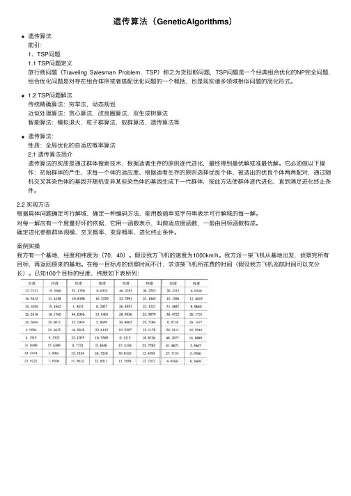
遗传算法（GeneticAlgorithms）遗传算法前引：1、TSP问题1.1 TSP问题定义旅⾏商问题（Traveling Salesman Problem，TSP）称之为货担郎问题，TSP问题是⼀个经典组合优化的NP完全问题，组合优化问题是对存在组合排序或者搭配优化问题的⼀个概括，也是现实诸多领域相似问题的简化形式。

1.2 TSP问题解法传统精确算法：穷举法，动态规划近似处理算法：贪⼼算法，改良圈算法，双⽣成树算法智能算法：模拟退⽕，粒⼦群算法，蚁群算法，遗传算法等遗传算法：性质：全局优化的⾃适应概率算法2.1 遗传算法简介遗传算法的实质是通过群体搜索技术，根据适者⽣存的原则逐代进化，最终得到最优解或准最优解。

它必须做以下操作：初始群体的产⽣、求每⼀个体的适应度、根据适者⽣存的原则选择优良个体、被选出的优良个体两两配对，通过随机交叉其染⾊体的基因并随机变异某些染⾊体的基因⽣成下⼀代群体，按此⽅法使群体逐代进化，直到满⾜进化终⽌条件。

2.2 实现⽅法根据具体问题确定可⾏解域，确定⼀种编码⽅法，能⽤数值串或字符串表⽰可⾏解域的每⼀解。

对每⼀解应有⼀个度量好坏的依据，它⽤⼀函数表⽰，叫做适应度函数，⼀般由⽬标函数构成。

确定进化参数群体规模、交叉概率、变异概率、进化终⽌条件。

案例实操我⽅有⼀个基地，经度和纬度为（70，40）。

假设我⽅飞机的速度为1000km/h。

我⽅派⼀架飞机从基地出发，侦察完所有⽬标，再返回原来的基地。

在每⼀⽬标点的侦察时间不计，求该架飞机所花费的时间（假设我⽅飞机巡航时间可以充分长）。

已知100个⽬标的经度、纬度如下表所列:3.2 模型及算法求解的遗传算法的参数设定如下：种群⼤⼩M=50；最⼤代数G=100;交叉率pc=1，交叉概率为1能保证种群的充分进化；变异概率pm=0.1，⼀般⽽⾔，变异发⽣的可能性较⼩。

编码策略:初始种群：⽬标函数：交叉操作：变异操作：选择：算法图：代码实现：clc,clear, close allsj0=load('data12_1.txt');x=sj0(:,1:2:8); x=x(:);y=sj0(:,2:2:8); y=y(:);sj=[x y]; d1=[70,40];xy=[d1;sj;d1]; sj=xy*pi/180; %单位化成弧度d=zeros(102); %距离矩阵d的初始值for i=1:101for j=i+1:102d(i,j)=6370*acos(cos(sj(i,1)-sj(j,1))*cos(sj(i,2))*...cos(sj(j,2))+sin(sj(i,2))*sin(sj(j,2)));endendd=d+d'; w=50; g=100; %w为种群的个数，g为进化的代数for k=1:w %通过改良圈算法选取初始种群c=randperm(100); %产⽣1，...，100的⼀个全排列c1=[1,c+1,102]; %⽣成初始解for t=1:102 %该层循环是修改圈flag=0; %修改圈退出标志for m=1:100for n=m+2:101if d(c1(m),c1(n))+d(c1(m+1),c1(n+1))<...d(c1(m),c1(m+1))+d(c1(n),c1(n+1))c1(m+1:n)=c1(n:-1:m+1); flag=1; %修改圈endendendif flag==0J(k,c1)=1:102; break %记录下较好的解并退出当前层循环endendendJ(:,1)=0; J=J/102; %把整数序列转换成[0,1]区间上实数即染⾊体编码for k=1:g %该层循环进⾏遗传算法的操作for k=1:g %该层循环进⾏遗传算法的操作A=J; %交配产⽣⼦代A的初始染⾊体c=randperm(w); %产⽣下⾯交叉操作的染⾊体对for i=1:2:wF=2+floor(100*rand(1)); %产⽣交叉操作的地址temp=A(c(i),[F:102]); %中间变量的保存值A(c(i),[F:102])=A(c(i+1),[F:102]); %交叉操作A(c(i+1),F:102)=temp;endby=[]; %为了防⽌下⾯产⽣空地址，这⾥先初始化while ~length(by)by=find(rand(1,w)<0.1); %产⽣变异操作的地址endB=A(by,:); %产⽣变异操作的初始染⾊体for j=1:length(by)bw=sort(2+floor(100*rand(1,3))); %产⽣变异操作的3个地址%交换位置B(j,:)=B(j,[1:bw(1)-1,bw(2)+1:bw(3),bw(1):bw(2),bw(3)+1:102]);endG=[J;A;B]; %⽗代和⼦代种群合在⼀起[SG,ind1]=sort(G,2); %把染⾊体翻译成1，...,102的序列ind1num=size(G,1); long=zeros(1,num); %路径长度的初始值for j=1:numfor i=1:101long(j)=long(j)+d(ind1(j,i),ind1(j,i+1)); %计算每条路径长度endend[slong,ind2]=sort(long); %对路径长度按照从⼩到⼤排序J=G(ind2(1:w),:); %精选前w个较短的路径对应的染⾊体endpath=ind1(ind2(1),:), flong=slong(1) %解的路径及路径长度xx=xy(path,1);yy=xy(path,2);plot(xx,yy,'-o') %画出路径以上整个代码中没有调⽤GA⼯具箱。