On the Determinants of Measurement Error in Time-Driven Costing

CE
美国卫生及公共服务部食品药品管理局（- GE Medical Systems SCS
VA Preferences
引言
此标志表示潜在的危险状况，如果没有避免可导致较小的
图像要求
左心室工作流程
Navigator EP
3
Coronary Sinus Analysis
使用鼠标右键单击中心线
肺部血管分析
重构协议
心脏重构
短轴长轴垂直长轴
心脏特殊查看功能
相位注册
快速
狭窄工具
视图和控制内腔
Branch
围绕中心线的旋转角度 血管分支 视图类型 复制模式 （Rfmt 或MIP ）
从中心线开始的光标线性位置
窗宽/窗位
曲线类型
（截面积或平均直径）
光标线
图表
患者姓名
内腔条的宽度
视图上的菜单
测量。

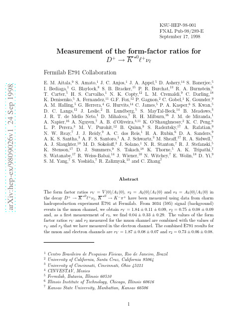
a r X i v :h e p -e x /9809026v 1 24 S e p 1998KSU-HEP-98-001FNAL Pub-98/289-E September 17,1998Measurement of the form-factor ratios forD +→K⋆0ℓ+νℓ,1Centro Brasileiro de Pesquisas F´ısicas,Rio de Janeiro,Brazil 2University of California,Santa Cruz,California 950643University of Cincinnati,Cincinnati,Ohio 452214CINVESTAV,Mexico5Fermilab,Batavia,Illinois 605106Illinois Institute of Technology,Chicago,Illinois 606167Kansas State University,Manhattan,Kansas 665068University of Massachusetts,Amherst,Massachusetts010039University of Mississippi,University,Mississippi3867710Princeton University,Princeton,New Jersey0854411Universidad Autonoma de Puebla,Mexico12University of South Carolina,Columbia,South Carolina2920813Stanford University,Stanford,California9430514Tel Aviv University,Tel Aviv,Israel15Box1290,Enderby,BC,V0E1V0,Canada16Tufts University,Medford,Massachusetts0215517University of Wisconsin,Madison,Wisconsin5370618Yale University,New Haven,Connecticut06511K⋆0ℓ+νℓare an especially clean way to study these effects because the leptonicand hadronic currents completely factorize in the decay amplitude.All informa-tion about the strong interactions can be parametrized by a few form factors.Also, according to Heavy Quark Effective Theory,the values of form factors for somesemileptonic charm decays can be related to those governing certain b-quark de-cays.In particular,the form factors studied here can be related to those for therare B–meson decays B→K⋆e+e−and B→K⋆γ[1,2]which provide windows for physics beyond the Standard Model.With a vector meson in thefinal state,there are four form factors,V(q2),A1(q2),A2(q2)and A3(q2),which are functions of the Lorentz-invariant momentum transfer squared[3].The differential decay rate for D+→K⋆0→K−π+is a quadratic homogeneous function of the four form factors.Unfortunately,the limited size of current data samples precludes precise measurement of the q2-dependence of the form factors;we thus assume the dependence to be given by the nearest-pole dominance model:F(q2)=F(0)/(1−q2/m2pole)where m pole= m V=2.1GeV/c2for the vector form factor V,and m pole=m A=2.5GeV/c2 for the three axial-vector form factors[4].The third form factor A3(q2),which is unobservable in the limit of vanishing lepton mass,probes the spin-0component of the off-shell W.Additional spin-flip amplitudes,suppressed by an overall factor of m2ℓ/q2when compared with spin no-flip amplitudes,contribute to the differential decay rate.Because A1(q2)appears among the coefficients of every term in the differential decay rate,it is customary to factor out A1(0)and to measure the ratios r V=V(0)/A1(0),r2=A2(0)/A1(0)and r3=A3(0)/A1(0).The values of these ratios can be extracted without any assumption about the total decay rate or the weak mixing matrix element V cs.We report new measurements of the form factor ratios for the muon chan-nel and combine them with slightly revised values of our previously publishedmeasurements of r V and r2[5]for the electron channel.This is thefirst set of measurements in both muon and electron channels from a single experiment.We also report thefirst measurement of r3=A3(0)/A1(0),which is unobservable in the limit of vanishing charged lepton mass.E791is afixed-target charm hadroproduction experiment[6].Charm particles were produced in the collisions of a500GeV/cπ−beam withfive thin targets, one platinum and four diamond.About2×1010events were recorded during the 1991-1992Fermilabfixed-target run.The tracking system consisted of23planes of silicon microstrip detectors,45planes of drift and proportional wire chambers, and two large-aperture dipole magnets.Hadron identification is based on the in-formation from two multicellˇCerenkov counters that provided good discrimination between kaons and pions in the momentum range6−36GeV/c.In this momentum range,the probabability of misidentifying a pion as a kaon depends on momentum but does not exceed5%.We identified muon candidates using a single plane of scintillator strips,oriented horizontally,located behind an equivalent of2.4meters of iron(comprising the calorimeters and one meter of bulk steel shielding).The an-gular acceptance of the scintillator plane was≈±62mrad×±48mrad(horizontally and vertically,respectively),which is somewhat smaller than that of the rest of the spectrometer for tracks which go through both magnets(≈±100mrad×±64mrad). The vertical position of a hit was determined from the strip’s vertical position,and the horizontal position of a hit from timing information.The event selection criteria used for this analysis are the same as for the electronic-mode form factor analysis[5],except for those related to lepton identifi-cation.Events are selected if they contain an acceptable decay vertex determined by the intersection point of three tracks that have been identified as a muon,a kaon,and a pion.The longitudinal separation between this candidate decay vertex and the reconstructed production vertex is required to be at least15times the esti-mated error on the separation.The two hadrons must have opposite charge.If the kaon and the muon have opposite charge,the event is assigned to the“right-sign”sample;if they have the same charge,the event is assigned to the“wrong-sign”sample used to model the background.To reduce the contamination from hadron decays inflight,only muon can-didates with momenta larger than8GeV/c are retained.With this momentum restriction,the efficiency of muon tagging was about85%,and the probability for a hadron to be identified as a muon was about3%.To exclude feedthrough from D+→K−π+π+,we exclude events in which the invariant mass of the three charged particles(with the muon candidate interpreted as a pion)is consistent with the D+mass.For ourfinal selection criteria,we use a binary-decision-tree algorithm(CART[7]),whichfinds linear combinations of parameters that have the highest discrimination power between signal and ing this algorithm,we found a linear combination of four discrimination variables[5]:(a)separation significance of the candidate decay vertex from target material;(b)distance of closest approach of the candidate D momentum vector to the primary vertex,taking into account the maximum kinematically-allowedmiss distance due to the unobserved neutrino;(c)product over candidate D decay tracks of the distance of closest approach of the track to the secondary vertex, divided by the distance of closest approach to the primary vertex,where each dis-tance is measured in units of measurement errors;and(d)significance of separation between the production and decay vertices.Thisfinal selection criterion reduced the number of wrong-sign events by50%,and the number of right-sign events by 25%.Although this does not affect our sensitivity substantially,it does reduce systematic uncertainties associated with the background subtraction.The minimum parent mass M min is defined as the invariant mass of Kπµνwhen the neutrino momentum component along the D+direction offlight is ignored.The distribution of M min should have a Jacobian peak at the D+mass,and we observe such a peak in our data(Fig.1).We retain events with M min in the range1.6 to2.0GeV/c2as indicated by the arrows in thefigure.The distribution of Kπinvariant mass for the retained events is shown in the top right of Fig.1for both right-sign and wrong-sign samples.Candidates with0.85<M Kπ<0.94GeV/c2 were retained,yieldingfinal data samples of3629right-sign and595wrong-sign events.The hadroproduction of charm,the differential decay rate,and the detector response were simulated with a Monte Carlo event generator.A sample of events was generated according to the differential decay rate(Eq.22in Ref.[3]),with the form factor ratios r V=2.00,r2=0.82,and r3=0.00.The same selection criteria were applied to the Monte Carlo events as to real data.Out of25million generated events,95579decays passed all cuts.Figure1(bottom)shows the distribution of M Kπfrom real data after background subtraction(“right-sign”minus“wrong-sign”)overlaid with the corresponding Monte Carlo distribution after all cuts are applied.The agreement between the two distributions suggests that wrong-sign events correctly account for the size of the background.The differential decay rate[3]is expressed in terms of four independent kine-matic variables:the square of the momentum transfer(q2),the polar angleθV in theK⋆0and W+decay planes.The definition we use for the polar angle θℓis related to the definition used in Ref.[3]byθℓ→π−θℓ.Semileptonic decays cannot be fully reconstructed due to the undetected neu-trino.With the available information about the D+direction offlight and the charged daughter particle momenta,the neutrino momentum(and all the decay’s kinematic variables)can be determined up to a two-fold ambiguity if the parent mass is constrained.Monte Carlo studies show that the differential decay rate is more accurately determined if it is calculated with the solution corresponding to the lower laboratory-frame neutrino momentum.To extract the form factor ratios the distribution of the data points in the four-dimensional kinematic variable space isfit to the full expression for the differential decay rate.We use the same unbinned maximum-likelihoodfitting technique as inour D+→K⋆0µ+νµcandidates as the previous method, but uses additional neutrino-momentum solutions.This is true for both the data and for the Monte Carlo sample used in the likelihood function calculation,so the results of thisfit could differ from those of the previousfit.The values of the form factor ratios obtained with the two methods agree well, providing further assurance that selecting the lower neutrino momentum solution in the primary method and correcting for the systematic bias gives the correct result.However,the systematic uncertainties for the primary method(see below) were found to be significantly smaller,mainly because the unbinned maximum-likelihood method is more stable against changes in the size of the phase spacevolume.Therefore,the primary method was chosen for quotingfinal results.We classify systematic uncertainties into three categories:(a)Monte Carlo simulation of detector effects and production mechanism;(b)fitting technique;(c) background subtraction.The estimated contributions of each are given in Table I. The main contributions to category(a)are due to muon identification and data selection criteria.The contributions to category(b)are related to the limited size of the Monte Carlo sample and to corrections for systematic bias.The measurements of the form factor ratios for D+→K⋆0e+νe[5]follow the same analysis procedure except for the charged lepton identification.Both results are listed in Table II.The consistency within errors of the results measured in the electron and muon channels supports the assumption that strong interaction effects,incor-porated in the values of form factor ratios,do not depend on the particular W+ leptonic decay.Based on this assumption,we combine the results measured for the electronic and muonic decay modes.The averaged values of the form factor ratios are r V=1.87±0.08±0.07and r2=0.73±0.06±0.08.The statistical and systematic uncertainties of the average results were determined using the general procedure described in Ref.[9](Eqns.3.40and3.40′).Some of the systematic errors for the two samples have positive correlation coefficients,and some nega-tive.The combination of all systematic errors is ultimately close to that which one would obtain assuming all the errors are uncorrelated.The third form factor ratio r3was not measured in the electronic mode.Table II compares the values of the form factor ratios r V and r2measured by E791in the electron,muon and combined modes with previous experimental results.The size of the data sample and the decay channel are listed for each case. All experimental results are consistent within errors.The comparison between the E791combined values of the form factor ratios r V and r2and previous experimental results is also shown in Fig.3(top).Table III and Fig.3(bottom)compare thefinal E791result with published theoretical predictions.The spread in the theoretical results is significantly larger than the E791experimental errors.To summarize,we have measured the values of the form factor ratios in the decay channel D+→K⋆0e+νe gives r V=1.87±0.08±0.07and r2=0.73±0.06±0.08.We gratefully acknowledge the assistance from Fermilab and other participat-ing institutions.This work was supported by the Brazilian Conselho Nacional de Desenvolvimento Cient´ıfico e Technol´o gico,CONACyT(Mexico),the Israeli Academy of Sciences and Humanities,the U.S.Departament of Energy,the U.S.-Israel Binational Science Foundation,and the U.S.National Science Foundation.REFERENCES[1]N.Isgur and M.B.Wise,Phys.Rev.D42(1990)2388.[2]Z.Ligeti,I.W.Stewart and M.B.Wise,Phys.Lett.B420(1998)359.[3]J.G.K¨o rner and G.A.Schuler,Phys.Lett.B226(1989)185.[4]Particle Data Group,Review of Particle Physics,Phys.Rev.D50(1994)1568.[5]Fermilab E791Collaboration,E.M.Aitala et al.,Phys.Rev.Lett.80(1998)1393.The E791electron result for r V quoted in this paper is0.06higher than the value reported in this reference because we have corrected for inaccuracies in the earlier modeling of the D+transverse momentum.[6]J.A.Appel,Ann.Rev.Nucl.Part.Sci.42(1992)367;D.J.Summers et al.,XXVII Rencontre de Moriond,Les Arcs,France(15-22March1992)417. [7]L.Brieman et al.,Classification and Regression Trees(Chapman and Hall,New York,1984).[8]D.M.Schmidt,R.J.Morrison,and M.S.Witherell,Nucl.Instrum.Methods A328(1993)547.[9]L.Lyons,Statistics for Nuclear and Particle Physicists(Cambridge UniversityPress,Cambridge,1986).[10]Fermilab E687Collaboration,P.L.Frabetti et al.,Phys.Lett.B307(1993)262.[11]Fermilab E653Collaboration,K.Kodama et al.,Phys.Lett.B274(1992)246.[12]Fermilab E691Collaboration,J.C.Anjos et al.,Phys.Rev.Lett.65(1990)2630.[13]D.Scora and N.Isgur,Phys.Rev.D52(1995)2783.We have used the q2-dependence assumed in thefits to our data to extrapolate the theoretical form factors from q2=q2max to q2=0.[14]M.Wirbel,B.Stech,and M.Bauer,Z.Phys.C29(1985)637.[15]T.Altomari and L.Wolfenstein,Phys.Rev.D37(1988)681.[16]F.J.Gilman and R.L.Singleton,Jr.,Phys.Rev.D41(1990)142.[17]B.Stech,Z.Phys.C75(1997)245.[18]C.W.Bernard,Z.X.El-Khadra,and A.Soni,Phys.Rev.D45(1992)869,Phys.Rev.D47(1993)998.[19]V.Lubicz,G.Martinelli,M.S.McCarthy,and C.T.Sachrajda,Phys.Lett.B274(1992)415.[20]A.Abada et al.,Nucl.Phys.B416(1994)675.[21]C.R.Alton et al.,Phys.Lett.B345(1995)513.[22]K.C.Bowler et al.,Phys.Rev.D51(1995)4905.[23]P.Ball,V.M.Braun,and H.G.Dosch,Phys.Rev.D44(1991)3567.[24]T.Bhattacharya and R.Gupta,Nucl.Phys.B(Proc.Suppl.)47(1996)481.TABLESTABLE I.The main contributions to uncertainties on the form factor ratios.Sourceσr2σrVσr3Hadron identification0.010.010.02 Muon identification0.040.060.10 Production mechanism0.010.010.02 Acceptance0.030.020.08 Cut selection0.030.040.09MC volume size0.020.020.12 Number of MC points0.010.010.18 Bias0.010.020.06No.of background events0.040.020.06 Background shape0.040.040.06 E7916000(e+µ)1.87±0.08±0.070.73±0.06±0.08 E7913000(µ)1.84±0.11±0.090.75±0.08±0.09 E7913000(e)1.90±0.11±0.090.71±0.08±0.09 E687[10]900(µ)1.74±0.27±0.280.78±0.18±0.10E653[11]300(µ)2.00+0.34−0.32±0.160.82+0.22−0.23±0.11E691[12]200(e)2.0±0.6±0.30.0±0.5±0.2TABLE parison of E791results with theoretical predictions for the form factor ratios r V and r2.Group r V r2ISGW2[13]2.01.3WSB[14]1.41.3KS[3]1.01.0AW/GS[15,16]2.00.8Stech[17]1.551.06BKS[18]1.99±0.22±0.330.70±0.16±0.17 LMMS[19]1.6±0.20.4±0.4ELC[20]1.3±0.20.6±0.3APE[21]1.6±0.30.7±0.4UKQCD[22]1.4+0.5−0.20.9±0.2BBD[23]2.2±0.21.2±0.2 LANL[24]1.78±0.070.68±0.11FIGURES01002003004005006001.251.51.7522.25M min (GeV/ c 2)E v e n t s / 40 M e V / c21002003004005006007000.70.80.91 1.1K π invariant mass (GeV/ c 2)E v e n t s / 10 M e V / c 2050100150200250300K π invariant mass (GeV/ c 2)E v e n t s / 5 M e V / c2FIG.1.Distributions of minimum parent mass M min and Kπinvariant mass for D +→050100150200cos θl (q 2/q 2max < 0.5)E v e n t s / 0.2050100150200cos θl (q 2/q 2max ≥ 0.5)E v e n t s / 0.250100150200cos θV (q 2/q 2max < 0.5)E v e n t s / 0.2050100150200cos θV (q 2/q 2max ≥ 0.5)E v e n t s / 0.250100150200χ (cos θV < 0)E v e n t s / 0.2π050100150200χ (cos θV ≥ 0)E v e n t s / 0.2πparison of single-variable distributions of background-subtracted data (crosses)with Monte Carlo predictions (dashed histograms)using best-fit values for the form factor ratios.1111.21.41.61.822.22.4rr V11.21.41.61.822.22.4r 2r VFIG.3.Top:Comparison of experimental measurements of form factor ratios r V and r 2for D +→。

k = correlation coefficient 相关系数SD = standard deviation 标准偏差RSD = relative standard deviation相对标准偏差The following qualification tests may also be performed in addition to those described in Table 3 (recommended, not obligatory): 表3中可能还需有以下确认内容（推荐，非强制）：7. QUALIFICATION PROCEDURE 确认程序Verification 验证Verification of the balance is performed by placing a suitable weight (depending on the typeof balance) in the centre of the weighing pan once and comparing the result with pre-defined acceptance criteria. The same weight should always be used in these verifications.天平的验证是通过将适当的砝码（根据天平的类型选择）放置在秤盘中心测定，结果与预先设定的标准进行比较。

在验证中应一直使用相同的砝码。

The acceptance criteria shall be defined by each individual OMCL.每个实验室自行制订可接受标准。

Accuracy准确度The accuracy of the balance is checked by weighing at least three different certified weightsthat cover the usual weighing range of the balance. It is recommended that the weights have approximately 5%, 50% and 100% of the maximum capacity of the balance (or of the maximum weight used on the balance), depending on the type of balance. It is recommended that the weighing is repeated at least 5 times for every weight, particularly, when the results shall also be used in the test for precision.天平的准确度应至少由三个不同的标准砝码进行检查，应涵盖天平的通常称量范围。

Re-examination of Physical Models in theTemperature Range300K–700KAndreas Schenk1Technical Report No.99/011This work was supported by the German Bundesministerium für Bildung und Forschung under contract01M3034A.The authors are responsible for the contents of this publication.AbstractIn the PARASITICS project physical models used in device simulation are to be verified for the temperature range300K–700K(lattice temperature)by compari-son between simulation and electrical characterization of suitable test structures.A pre-evaluation of the decisive models in DESSIS ISE showed good agreement with existing experimental data up to500K and normal physical behavior up to1000K. The mobility model of Schenk[1]wasfine-tuned by means of a careful analysis of all existing data on the temperature dependence of the mobility.Drift velocity satu-ration is now perfectly reproduced for both electrons and holes,provided the energy relaxation times are given the valuesτE n075ps,τE p017ps in the simulation.A complete device analysis of DIODE24_BL from MOD_B_BOSCH based on dop-ing profiles by ST and measured IV-characteristics in the temperature range300K –700K with the device simulator DESSIS ISE produced the following results:At all temperatures the forward-bias range is dominated by SRH recombination up to a current of1105A,and by trap-assisted Auger(TAA)recombination above.The latter is the sum of temperature-dependent contributions from p-region,n-region, and buried layer.The measured temperature dependence of the high-injection range of the IV-curves is possibly due to the TAA coefficients,which could not be worked out since DESSIS ISE did not converge there.All alternative possibilities-band gap,carrier statistics,BGN model,surface recombination,and band-to-band Auger recombination could be systematically ruled out.The temperature dependence of the reverse-bias IV-curves results from the changing contributions of p-region,n-region,and buried layer,respectively,to the total SRH generation ing thefit parameters of the lifetime models in DESSIS ISE,reasonable overall agreement was achieved without any hypothetical temperature dependence of the minority carrier lifetimes.A good match to the measured breakdown voltages was obtained for all temperatures with a modification of the vanOverstraeten model of the impact ioniza-tion coefficient of the formαconstγE g300KFE g TZusammenfassungZiel des Projekts ist die Verifizierung der physikalischen Modelle im Temperaturbe-reich300K–700K(Gittertemperatur)durch Vergleich von Simulation und elektri-scher Charakterisierung geeigneter Teststrukturen.Dazu wurden im V orfeld die wichtigsten Modelle in DESSIS ISE auf ihr Verhalten bis1000K Gittertemperatur hin untersucht.Alle Modelle zeigten guteÜbereinstimmung mit vorhandenen Mess-ergebnissen(bis max.500K)sowie normales physikalisches Verhalten bis1000K.Ein Schwerpunkt des Projekts ist der Test des physik-basierten Silizium Bulk-Beweglichkeitsmodells von Schenk[1]bei hohen Temperaturen.Zur V orbereitung der Hochtemperatur-Hall-Messungen wurde das Modell mit sämtlichen vorhande-nen Messungen der Abhängigkeit von Gitter-und Ladungsträgertemperatur ver-glichen.Die existierenden Datenüber die Sättigung der Driftgeschwindigkeit(bis max.370K)wurden benutzt,um eine Feinanpassung der funktionalen Form zu erhalten,nach der sich perfekte Sättigung der Driftgeschwindigkeit für Elektronen und Löcher ergibt.Die optimalen Energie-Relaxationszeiten für die beste Anpas-sung an experimentelle Daten wurden ermittelt(τE n075ps,τE p017ps).Die benötigten Hall-Faktoren bis700K für alle relevanten Dotierungen der im Projekt gegebenen Teststrukturen wurden bereitgestellt.Eine vollständige Bauelemente-Analyse der DIODE24_BL von MOD_B_BOSCH (laterale pPlus/nWell smart-power Diode)wurde basierend auf Dotierprofilen von ST und Kennlinien-Messungen im Temperaturbereich300K–700K mit dem Bauele-mente-Simulator DESSIS ISE durchgeführt.Wegen der grossen Komplexität dieses Bauelements(laterale pn-Übergänge,Durchbruch an der Si-SiO2-Grenzfläche, hochdotierte vergrabene Schicht)sind die Ergebnisse mit gewissen Unsicherheiten behaftet.Sie setzen insbesondere voraus,dass die lateralen Dotierprofile korrekt sind und der Avalanche-Durchbruch nicht wesentlich durch die Grenzfläche beeinflusst wird.Die Analyse der V orwärts-Kennlinien erbrachte folgende Resultate:SRH-Re-kombination dominiert bis zu einer Stromstärke von1105A im gesamten Tem-peraturbereich,wobei der Beitrag des n-Gebiets mit steigender Temperatur zunimmt. Oberhalb1105A ist trap-assistierte Auger-Rekombination(TAA)der einzig wichtige Rekombinationsmechanismus,wobei in Abängigkeit von der Temperatur alle drei Gebiete–p-Gebiet,n-Gebiet und vergrabene Schicht–Anteile liefern. Band-Band-Auger-Rekombination würde um drei Grössenordnungen zu grosse Auger-Koeffizienten erfordern.Die starke Temperatur-Abhängigkeit der Kennli-nien im Hochinjektionsbereich könnte nurüber die TAA-Koeffizienten erklärt wer-den.Eine entsprechende Anpassung konnte jedoch nicht erfolgen,weil DESSIS ISE in diesem Bereich nicht konvergierte.Sämtliche alternativen Möglichkeiten für den gemessenen Temperatur-Einfluss–Energielücke,Ladungsträgerstatistik,BGN-Modell und Oberflächen-Rekombination–konnten systematisch ausgeschlossen werden.Die Dominanz der TAA-Rekombination resultiert aus der Tatsache,dass die Implantation der vergrabenen Schicht ein voluminöses Gebiet mit sowohl ho-her Elektronendichte(was einen Auger-Prozess begünstigt)als auch mit hoher Trap-Dichte erzeugt(was einen SRH-Prozess begünstigt).Die V orwärts-Kennlinien sind demnach wesentlich durch Eigenschaften der vergrabenen Schicht bestimmt.Die Temperatur-Abhängigkeit der Sperrströme ist durch die wechselndenBeiträge der einzelnen Gebiete–p n-Übergang,n-Gebiet und vergrabene Schicht –zur totalen SRH-Rate bestimmt.Eine genaue Anpassung würde die Kenntnis der Lebensdauerprofile im gesamten Bauelement erfordern.Jedoch gelingt bereits mit sinnvollen Variationen der Lebensdauer-Modellparameter eine gute Simula-tion der Sperrströme,ohne jegliche(hypothetische)Temperatur-Abhängigkeit der Minoritätsladungsträgerlebensdauern.Insbesondere kann die charakteristischeÄn-derung der Form der Sperr-Kennlinien zu einem“rechteckigen"Verlauf ab etwa 350K erklärt werden.Die Durchbruchspannungen bei hohen Temperaturen können zwanglos mit dem Lokalfeldmodell der Stossionisationsrate simuliert werden,wenn für die Schwellenenergie die temperaturabhängige Energielücke benutzt wird.Diese wurde ins vanOverstraeten-Modell implementiert,so dass sichαconstγE g300KFE g TFigure1:Temperature dependence of the indirect band gap in silicon.See the DESSIS ISE manual for the E g T L formula.Figure2:Impact ionization coefficient for electrons as function of electricfield as it turns out from Lackner’s model.given by the band gap and,therefore,should exhibit the(strong)temperature depen-dence of the latter.This will be detailed below.The drift velocity saturation for electrons at different lattice temperatures from Canali’s model[2],(p.65)is shown in Fig.3.It decreases with rising temperature at afixedfield strength in the Ohmic regime.In the saturation range the spacing between different curves becomes narrower with increasing temperature.This indicates that the relative decrease of the saturation velocity declines at higher temperatures.Figure3:Electron drift velocity as function of electricfield for different lattice tem-peratures as it turns out from Canali’s model.In Fig.4the bulk mobility of Schenk[2],(p.127)is compared with the DESSIS ISE default model and experimental data in the entire temperature range up to1000K.Despite the good coincidence,the range between500K and1000K requires further investigations.The physics-based Schenk mobility model allows conclusions about the scatter-ing of hot carriers in doped(bulk)silicon.Fig.5depicts the electron mobility as function of the electricfield at different doping levels.In the300K case an inter-esting behavior is observed which can be explained as follows:When the carrier temperature reaches a certain value,the Coulomb scattering at ionized dopants be-comes less important and the mobility increases.Further carrier heating,however, immediately leads to the common saturation effect due to the balance between en-ergy gain by the electricfield and energy loss by emission of optical phonons.At the highest doping concentrations,the increase of the mobility only sets in after velocity saturation had already started to be effective.The latter behavior was only found for electrons but not for holes.In the right part of Fig.5results for700K are shown on the same scale.One observes that at high lattice temperatures the described effects do not occur because the saturation mechanism dominates.Figure4:Electron bulk mobility as function of lattice temperature as it turns out from Schenk’s model compared to experimental data and the DESSIS ISE default model.Figure5:Electron bulk mobility as function of electricfield for different doping concentrations as it turns out from Schenk’s model.Left:T L300K,right:T L 700K2Drift velocity saturation in Schenk’s bulk mobility model2.1Simulation of n-type resistorIt is commonly believed that the drift velocity in bulk silicon perfectly saturates both in the case of electrons and holes,if the local electricfield exceeds2105V/cm.Thebulk mobility model as published in Ref.[1]was slightly modified to reproduce this perfect velocity saturation.For this,the integral factor I ac T c2112αk B T c in the expressions describing phonon scattering had to be changed to2Figure7:Electron drift velocity at room temperature.Experimental data points arefor different substrate orientations(100or111).(blue curve).The red curve represents the result of the terminal extraction method which yields a perfectfit in the Ohmic regime(this has to be so,since deformationpotentials and phonon energies had beenfixed to reproduce the Ohmic mobility).The above mentioned effect of carrier injection becomes visible at approximately4103V/cm.If the third method is applied,the red curve merges with the blue one at about1104V/cm.From this exercice we draw the conclusion that the only change to be made in theset of parameters is the choiceτE n075ps.2.2Simulation of p-type resistorExchanging n by p in Fig.6defines the p-type resistor used to optimize the param-eters for the hole drift velocity.In Fig.8the green curve again represents the resultobtained with default values.In order to match the data of Smith,αp would have to be further reduced.However,the low valueαp015eV1had already been a concession to a reasonablefit of the drift velocity in Ref.[1].The bestfit of the holeDOS was found withαp05eV1.Therefore,we better leave the nonparabolicity parameter untouched and adjust the energy relaxation timeτE p as above(blue and black curves).A reasonable agreement with the scattering experimental data is found usingτE p017ps or larger(up to0.20ps).It is impossible to reproduce the sharp saturation behavior found by Smith[4].As in the case of electrons,the terminal extraction method gives a perfectfit in the Ohmic regime.We conclude thatαp05eV1andτE p017ps are the best choice and henceFigure8:Hole drift velocity at room temperature.will be used in the high-temperature investigations.2.3Comparison with published data on ambient temperature de-pendenceThere exist a few published data for ambient temperatures different from room tem-perature.In Figs.9and10we show the drift velocities for245K and370K in com-parison to data by Canali et al[3].In the case of electrons the agreement is equally good using the same parameters as for room temperature.In the case of holes the 370K curvefits very well with the same parameters that have been found for300K, whereas for the lower temperature a larger misfit occurs.Increasing the energy re-laxation time would improve the situation,however it seems to be more likely that the misfit is related to the use of an effective hole mass which strongly depends on temperature in DESSIS ISE.We already argued in Ref.[2],(p.163)that the T L-dependence of the hole DOS mass should not be used for transport calculations.3DIODE24_BL from MOD_B_BOSCH3.12D default simulationA cross section of the planar diode DIODE24_BL(pPlus/nWell)together with a zoom into the critical region are shown in Fig.11.Avalanche breakdown occurs in small areas on both sides of the p n junction just below the Si-SiO2interface.Figure9:Electron drift velocity versus electricfield for different lattice temperatures.Figure11:2D cross section of the smart-power diode DIODE24_BL.The insetshows the distribution of the impact ionization rate at breakdown.The maxima of the rate are located directly underneath the surface.The simulationof the breakdown voltage and the evaluation of the impact ionization model at hightemperatures hence will be obscured by the uncertainty from the lateral doping profile and the possible existence of a surface channel for breakdown.In the following wehave to assume that DIODE24_BL is nevertheless a suitable test device.Dopingprofile and electricfield across the critical region are shown in Fig.12.Thefieldvariation is about20%over a distance of100nm which is smooth enough to justify the application of a local-field model.The default simulation of the forward and reverse IV-characteristics is defined asfollows:SRH(minority carrier)lifetimes independent on doping and temperature,fixed toτn14106s,τp42107s for the bestfit to the SRH-dominated branch of the298K forward IV-curve.Recombination processes are“Auger"(de-fault parameters including the T-dependence of the Auger coefficients)and“SRH",BGN model is“slotboom",the statistics is“Boltzmann-Maxwell"(i.e.“Fermi"notswitched on).Electron-hole scattering(“carrier-carrier",Brooks-Herring)has to be included for a correct curvature in the bias range-0.8V–-1V where plasma ef-fects play an important role.Generation processes are“SRH"and impact ioniza-tion(“vanOverstraeten").The criticalfields in the Chynoweth law were lowered by5%in order to match the measured breakdown voltage at323K:b n lowFigure12:Doping concentration and electricfield profile at zero bias across the p n junction near the surface.Figure13:Default simulation and measured forward IV-characteristics.The hori-zontal red line connects the built-in potentials for each temperature.11695106V/cm,b p low19342106V/cm,b n high11695106V/cm, b p high16083106V/cm.This can be considered as a concession to the above mentioned uncertainties induced by the lateral doping profile and the proximity of the surface.We assume that those effects,if present,have at the most a weak temperature dependence that can be neglected.Figure14:Built-in potential and free carrier densities in the depletion zone at zero bias.In the right legend n pl denotes the extracted plasma density(n=p).The forward and reverse IV-characteristics in the temperature range298K–699K are presented in Figs.13and15,respectively.Since the intrinsic density of silicon at700K is about3361016cm3,a main feature is the transition from the extrinsic to the intrinsic regime at some elevated temperature(depending on the local doping concentration).In the forward-bias range we observe that SRH recombina-tion dominates up to a current of1105A for all temperatures.Then some Auger process starts to dominate(either band-to-band(b2b)Auger or trap-assisted Auger (TAA))which also defines the onset of a remarkable deviation of the simulated from the measured current.This deviation extends up to-1V and covers the entire bias range at the highest temperatures.SRH recombination is completely masked in the range550K–700K.Hence the forward-bias branch is not suitable to draw any con-clusions about a temperature dependence of the SRH lifetimes.The shrinkage of the built-in potential with increasing temperature is depicted in Fig.14.If the built-in potential is marked on each corresponding curve in Fig.13,one obtains an almost horizontal line.In Fig.14it is also shown how a plasma develops in the depletion zone with rising T(plasma density n pl n p equal to the intrinsic density n i).One can see that above600K the electron density in the neutral n-region exceeds the doping,which results in the above-mentioned intrinsic behavior.Afirst inspection of the reverse-bias characteristics in Fig.15shows two fea-tures:the strong overestimation of the SRH-dominated current between323K and 450K,and far too large breakdown voltages for the higher temperatures.Below 11011A the experimental data turn into noise and are disregarded.A closer look on various quantities near breakdown at323K and648K,respectively,reveals someFigure15:Default simulation and measured reverse IV-characteristics. interesting aspects.In Fig.16electricfield and ionization rate across the junctionare compared for the two temperatures.Since the maxima of thefield are not muchdifferent from each other,the exponential function in the Chynoweth law produces a factor2difference at the most.However,the ionization rates differ by more thanfour orders of magnitude(37104)!This large difference is caused by theplasma density in the“depletion"region.(The impact ionization rate has the formG IIαn nv nαp pv p.)As indicated in the left part of Fig.17,the plasma has a density of about281012cm3at648K,a factor of62104larger than in thecase of323K.On the other hand,this plasma density is much smaller than the intrin-sic density at648K,which is about121016cm3.As the temperature increases,the SRH rate extends into the entire n-region because n ifirst approaches the electron density there,andfinally it determines the electron density.3.2Forward-bias analysisTo understand the physics behind the forward IV-characteristics it is useful to plot the dominant recombination processes.In Figs.18and19we present the profiles of the Auger and SRH rates along a vertical cut through the device that also covers the buried layer(BL).These profiles are shown for the two limiting temperatures and for three forward biases.In the right part of thefigures the integrated rates as a functionFigure16:Electricfield and impact ionization rate across the junction for two tem-peratures.Figure17:Free carrier densities at breakdown(left)and SRH rate at+12V bias (right)across the junction for different temperatures.of distance from the surface yield information about the relative contribution from different regions.At298K the Auger rates are concentrated in the p-region and the integrated Auger rate collects only very small contributions from the BL.The SRHFigure18:Profiles of the Auger and SRH rates at298K for V bias=-0.2V,-0.6V,and -1.0V from bottom to top(left).Integrated rates as a function of distance from the p-contact(right).Figure19:Profiles of the Auger and SRH rates at699K for V bias=-0.2V,-0.6V,and -1.0V from bottom to top(left).Integrated rates as a function of distance from the p-contact(right).rate exhibits the usual peak in the depletion zone which disappears as the built-in voltage becomes zero.At high bias and high temperatures the SRH rate distribu-tion is broad.SRH recombination is outnumbered by Auger recombination between -0.6V and-1V(from the IV-curve wefind-0.66V).At699K Auger recombination dominates in the whole forward bias range,but the BL region yields some contri-butions.This confirms the remarks made in the previous section.The transition from SRH to Auger dominance is easily seen from a plot of the ideality factor for alltemperatures in Fig.20.Figure20:Ideality factor as function of ambient temperature.We can draw the following important conclusion.Currents larger than1105Aoriginate from an Auger-type recombination process.At lower temperatures its rate is concentrated in the p-contact region.Hence for b2b Auger R Auger C hhe p2n there,and since n isfixed by N A,a temperature effect can only be due to the minor-ity carrier density n or/and the Auger coefficient C hhe.Besides b2b Auger,a secondrecombination process is possible in this regime:trap-assisted Auger(TAA)recom-bination.TAA is a SRH-type recombination process where the energy difference between band edge and trap level is transfered to excited electrons/holes.TAA starts to exceed the thermal SRH rate when c n p1τSRH,where c is the TAA coef-ficient in DESSIS ISE.Then the TAA rate has a maximum in the p-contact region (like b2b Auger),but also a broad and large distribution in the entire n-region(like thermal SRH)giving the major contribution simply due to its large volume.In both regions the TAA rate turns into R TAA c pn!In order to understand the shape of the forward IV-curves and their temperature dependence,we have to care about the following issues:1.)The T-dependence of the band gap E g T as it influences n.2.)The effect of the carrier statistics,since it affects the T-dependence of the quasiFermi levels.3.)The BGN model,since it determines the minority carrier densities.4.)The size of C hhe,C eeh and the impact of their T-and n p-dependence.5.)The influence of surface recombination.6.)The role of TAA and a possible T-dependence of c.1.)A striking misfit between measured and simulated forward IV-curves is the wrongtemperature dependence highlighted in Fig.21.In order to check the influence of E g T the parameters in E g T were changed in such a way that the gap shrinkage was enhanced up to a reasonable limit guided by the experimental data in Fig.1.The resulting effect was far too weak to explain the discrepancy in Fig.21.2.)and3.)The carrier statistics and different BGN models have a strong impact on the minor-ity carrier ing any“traditional"BGN model in combination with Fermi statistics will give the same minority carrier density as without“Fermi"(a wanted feature in DESSIS ISE).To force Fermi statistics without neglecting BGN at all, the"schenk"BGN was used[5].Again,the distance between the298K and699K curves is not essentially changed.Figure21:The effect of carrier statistics and different BGN models on the tempera-ture dependence of the forward IV-characteristics.4.)The b2b Auger coefficients C hhe and C eeh were systematically increased neglecting their temperature dependence.As shown in Fig.22one can match the data points in the Auger-dominated range with values of the order10291028cm6s1.How-ever,such values are2-3orders of magnitude larger than the usual and well-accepted value of1031cm6s1.5.)The minority carrier density at the surface never exceeds1016cm3.Assuming v sur f104cm/s for the surface recombination velocity,the resulting rate of sur-face recombination is always much less than the integrated rates shown in the right part of Figs.18and19(at small forward bias and for the lower temperatures the mi-nority carrier density is very small).Therefore,surface recombination can be safely ignored.Figure22:Variation of the b2b Auger coefficients(frozen T-dependence)for298K, 398K,501K,and648K(from bottom to top).6.)The remaining thinkable process is TAA recombination[2],(p.80).Results for c11011and c51011cm3s1are presented in Fig.23.Termi-nation of simulated curves is caused by non-convergency of DESSIS ISE.With c51011cm3s1a goodfit for all temperatures could be obtained.c might have a similar temperature dependence as the b2b Auger coefficients(thought to be due to phonon-assistance),although the spread of the deep-level wave functions in k-space would relax momentum conservation restrictions.Unfortunately,no assess-ment about the temperature dependence of c can be made.That TAA recombination could be identified as the dominant recombination pro-cess is not surprising.The implantation of the BL both creates a large volume of high electron density in favor of an Auger process and a large density of deep-lying trap states in favor of a SRH process.Hence the device behavior under forward bias is practically determined by induced features from the BL.3.3Reverse-bias analysis3.3.1LifetimesThe pre-breakdown branches of the reverse-bias curves exhibit a change from a rounded shape at“low"temperatures to an almost rectangular shape at higher tem-peratures.The temperature dependence itself seems to be irregular when compared with the default simulation.To gain more insight into the measured behavior we plot the SRH rate at+12.5V along a vertical cross section through the device includingFigure23:Variation of the TAA coefficient c for298K,398K,and648K(from bottom to top).the BL region in Fig.24.Note that the volume of the outer region is huge com-Figure24:Profiles of the SRH rate at a bias of+12.5V along a vertical cut through the device from the p-contact to the pn-junction of the BL for various temperatures. Lifetime parameters were the same as in the previous section.pared to the volume of the p n depletion zone.At“low"temperatures the depleted p n-junction yields the major contributions,but at an intermediate temperature the outer region has a comparable share,whereas at the highest temperatures the BL part of the outer region dominates the SRH rate.This change in the relative contri-butions to the total SRH rate is essential to understand the reverse-bias IV-curves. The maximum doping in the BL is about81018cm3,far more than in the de-pleted p n-junction.Since the minority carrier lifetimes are strongly affected by the process conditions,in particular by implantations with a high dose,heavily doped re-gions have(much)smaller lifetimes which is expressed by the so-called Scharfetter relation(SRH(DopingDependence)in DESSIS ISE)[2],(p.73).The blue curves in Figs.26and27were obtained with the default parameter set including“DopingDe-pendence",i.e.the lifetime parameters“taumax"were set back to Dessis default.By chance,the agreement at323K is the same as before(compare Fig.15).Applying the Scharfetter relation we obtain pictures as in Fig.25where the SRH rate(left) and the hole lifetime(right)are shown for the“intermediate"temperature of348K.Figure25:Distributions of the SRH rate(left)and of the hole lifetime(right)through-out the device.One observes that the hole lifetime in the depletion zone of the p n-junction(blue region on the left side)is much larger(the color is orange!)than that in the BL region (green-blue area on the right side).Although the BL region is quasi-neutral,this leads to a total contribution to the SRH rate(yellow area on the left side)which is com-parable to the contribution from the highly depleted p n-junction.The qualitative difference in the curve shape is caused by the different speed at which the SRH rates reach their full size when the reverse bias is turned on.Since in the BL region n is always much larger than n1,the rate turns into R SRH N BL D p n2i e f fτBL p N BL D there.p decreases everywhere in the BL,but the denominator remains constant.In the p n-junction we have R SRH n p n2i e f fτpn p n n1τpn n p p1.n pin the numerator decreases,but also n and p in the denominator,i.e.it takes longerFigure26:Reverse-bias IV-curves with default lifetime parameters including“Dop-ingDependence"in SRH(blue solid lines)and with E trap015eV(red solid lines). to“switch on"the rate to its(large)maximum level in the p n-junction.Comparison of the398K default simulation with the measured data(the blue bold line in Fig.26)reveals that the transition to the BL-dominated generation hasalready occurred at this temperature in reality,but not in the simulation.One caneasily increase the relative contribution of the BL region e.g.by shifting the traplevel out of its mid gap position.In Fig.26we used E trap015eV which increases n1n i e f f exp E trap k B T and,therefore,decreases R SRH in the p n-junction but not much in the BL region.The resulting IV-curves are shown in red in Fig.26.At398K the shape of the curve is now more rectangular andfits better the measuredshape.On the other hand,one can play with the parameters of the Scharfetter relation to increase the importance of one particular region and,at the same time,to increase or decrease the total SRH rate.A perfectfit is not attainable because it would re-quire the knowledge of the different lifetime profiles in the p n-junction and the whole outer region,respectively.Fig.27shows the result if the power“al pha"in the Scharfetter relation is increased from1to1.5(red solid lines).Now all curves are shifted up giving a reasonable agreement between450K and700K.From these exercises we draw the conclusion that also the reverse-bias branch does not yield in-formation about the temperature dependence of the minority carrier lifetimes.Note, that the lifetime parameters“taumax"were not changed at all so far.For the fol-。

a rXiv:h ep-e x /246v116Feb2EUROPEAN ORGANIZATION FOR NUCLEAR RESEARCH CERN-EP/2000-022February 04,2000Measurements of Cross Sections and Forward-Backward Asymmetries at the Z Resonance and Determination of Electroweak Parameters The L3Collaboration Abstract We report on measurements of hadronic and leptonic cross sections and leptonic forward-backward asymmetries performed with the L3detector in the years 1993−95.A total luminosity of 103pb −1was collected at centre-of-mass energies √s ≈m Z ±1.8GeV which corresponds to 2.5million hadronic and 245thousand leptonic events selected.These data lead to a significantly improved determination of Z parameters.From the total cross sections,combined with our measurements in 1990−92,we obtain the final results:m Z =91189.8±3.1MeV ,ΓZ =2502.4±4.2MeV ,Γhad =1751.1±3.8MeV ,Γℓ=84.14±0.17MeV .An invisible width of Γinv =499.1±2.9MeV is derived which in the Standard Model yields for the number of light neutrino species N ν=2.978±0.014.Adding our results on the leptonic forward-backward asymmetries and the tau polarisation,the effective vector and axial-vector coupling constants of the neutral weak current to charged leptons are determined to be ¯g ℓV =−0.0397±0.0017and ¯g ℓA =−0.50153±0.00053.Includingour measurements of the Z →b ¯b forward-backward and quark charge asymmetries a value for theeffective electroweak mixing angle of sin 21IntroductionThe Standard Model(SM)of electroweak interactions[1,2]is tested with great precision by the experiments performed at the LEP and SLC e+e−colliders running at centre-of-mass energies,√on the treatment of the t-channel contributions in e+e−→e+e−(γ)and on technicalities of the fit procedures,respectively.2The L3DetectorThe L3detector[13]consists of a silicon microvertex detector[14],a central tracking chamber, a high resolution electromagnetic calorimeter composed of BGO crystals,a lead-scintillator ring calorimeter at low polar angles[15],a scintillation counter system,a uranium hadron calorime-ter with proportional wire chamber readout and an accurate muon spectrometer.Forward-backward muon chambers,completed for the1995data taking,extend the polar angle coverage of the muon system down to24degrees[16]with respect to the beam line.All detectors are installed in a12m diameter magnet which provides a solenoidalfield of0.5T in the central region and a toroidalfield of1.2T in the forward-backward region.The luminosity is measured using BGO calorimeters preceded by silicon trackers[10]situated on each side of the detector.In the L3coordinate system the direction of the e−beam defines the z direction.The xy, or rφplane,is the bending plane of the magneticfield,with the x direction pointing to the centre of the LEP ring.The coordinatesφandθdenote the azimuthal and polar angles.3Data AnalysisThe data collected between1993and1995are split into nine samples according to the year√and the centre-of-mass energy.Data samples atshowers are simulated with the GHEISHA[28]program.The performance of the detector, including inefficiencies and their time dependence as observed during data taking,is taken into account in the simulation.With this procedure,experimental systematic errors on cross sections and forward-backward asymmetries are minimized.4LEP Energy CalibrationThe average centre-of-mass energy of the colliding particles at the L3interaction point is calcu-lated using the results provided by the Working Group on LEP Energy[9].Every15minutes the average centre-of-mass energy is determined from measured LEP machine parameters,ap-plying the energy model which is based on calibration by resonant depolarisation[29].This model traces the time variation of the centre-of-mass energy of typically1MeV per hour.The average centre-of-mass energies are calculated for each data sample individually as luminosity weighted averages.Slightly different values are obtained for different reactions because of small differences in the usable luminosity.The errors on the centre-of-mass energies and their correlations for the1994data and for the two scans performed in1993and1995are given in form of a7×7covariance matrix in Table1.The uncertainties on the centre-of-mass energy for the data samples not included in this matrix,i.e.the1993and1995pre-scans,are18MeV and10MeV,respectively.Details of the treatment of these errors in thefits can be found in Appendix B.The energy distribution of the particles circulating in an e+e−-storage ring has afinite width due to synchrotron oscillations.An experimentally observed cross section is therefore a convolution of cross sections at energies which are distributed around the average value in a gaussian form.The spread of the centre-of-mass energy for the L3interaction point as obtained from the observed longitudinal length of the particle bunches in LEP is listed in Table2[9]. The time variation of the average energy causes a similar,but smaller,effect which is included in these numbers.All cross sections and forward-backward asymmetries quoted below are corrected for the energy spread to the average value of the centre-of-mass energy.The relative corrections on the measured hadronic cross sections amount to+1.7per mill(‰)at the Z pole and to−1.1‰and−0.6‰at the peak−2and peak+2energy,respectively.The absolute corrections on the forward-backward asymmetries are very small.The largest correction is−0.0002for the muon and tau peak−2data sets.The error on the energy spread is propagated into thefits,resulting in very small contributions to the errors of thefitted parameters(see Appendix B).The largest effect is on the total width of the Z,contributing approximately0.3MeV to its error.During the operation of LEP,no evidence for an average longitudinal polarisation of the electrons or positrons has been observed.Stringent limits on residual polarisation during lumi-nosity runs are set such that the uncertainties on the determination of electroweak observables are negligible compared to their experimental errors[30].The determination of the LEP centre-of-mass energy in1990−92is described in Refer-ences[31].From these results the LEP energy error matrix given in Table3is derived.5Luminosity MeasurementThe integrated luminosity L is determined by measuring the number of small-angle Bhabha interactions e+e−→e+e−(γ).For this purpose two cylindrical calorimeters consisting of arraysof BGO crystals are located on either side of the interaction point.Both detectors are dividedinto two half-rings in the vertical plane to allow the opening of the detectors duringfilling ofLEP.A silicon strip detector,consisting of two layers measuring the polar angle,θ,and one layer measuring the azimuthal angle,φ,is situated in front of each calorimeter to preciselydefine thefiducial volume.A detailed description of the luminosity monitor and the luminosity determination can be found in Reference[10].The selection of small-angle Bhabha events is based on the energy depositions in adjacentcrystals of the BGO calorimeters which are grouped to form clusters.The highest-energy cluster on each side is considered for the luminosity analysis.For about98%of the cases a hitin the silicon detectors is matched with a cluster and its coordinate is used;otherwise the BGOcoordinate is retained.The event selection criteria are:1.The energy of the most energetic cluster is required to exceed0.8E b and the energy onthe opposite side must be greater than0.4E b,where E b is the beam energy.If the energyof the most energetic cluster is within±5%of E b the minimum energy requirement onthe opposite side is reduced to0.2E b in order to recover events with energy lost in the gaps between crystals.The distributions of the energy of the most energetic cluster andthe cluster on the opposite side as measured in the luminosity monitors are shown in Figure1for the1993data.All selection cuts except the one under study are applied.2.The cluster on one side must be confined to a tightfiducial volume:•32mrad<θ<54mrad;|φ−90◦|>11.25◦and|φ−270◦|>11.25◦.The requirements on the azimuthal angle remove the regions where the half-rings of thedetector meet.The cluster on the opposite side is required to be within a largerfiducialvolume:•27mrad<π−θ<65mrad;|φ−90◦|>3.75◦and|φ−270◦|>3.75◦.This ensures that the event is fully contained in the detectors and edge effects in the reconstruction are avoided.3.The coplanarity angle∆φ=φ(z<0)−φ(z>0)between the two clusters must satisfy|∆φ−180◦|<10◦.The distribution of the coplanarity angle is shown in Figure2.Very good agreement with theMonte Carlo simulation is observed.Four samples of Bhabha events are defined by applying the tightfiducial volume cut to oneof theθ-measuring silicon layers.Taking the average of the luminosities obtained from thesesamples minimizes the effects of relative offsets between the interaction point and the detectors. The energy and coplanarity cuts reduce the background from random beam-gas coincidences.The remaining contamination is very small:(3.4±2.2)·10−5.This number is estimated using the sidebands of the coplanarity distribution,10◦<|∆φ−180◦|<30◦,after requiring that neither of the two clusters have an energy within±5%of E b.The accepted cross section is determined from Monte Carlo e+e−→e+e−(γ)samples gen-√erated with the BHLUMI event generator at afixed centre-of-mass energy ofs=91.25GeV the acceptedcross section is determined to be69.62nb.The statistical error on the Monte Carlo sample con-tributes0.35‰to the uncertainty of the luminosity measurement.The theoretical uncertainty on the Bhabha cross section in ourfiducial volume is estimated to be0.61‰[12].The experimental errors of the luminosity measurement are small.Important sources of systematic errors are:geometrical uncertainties due to the internal alignment of the silicon detectors(0.15‰to0.27‰),temperature expansion effects(0.14‰)and the knowledge on the longitudinal position of the silicon detectors(0.16‰to0.60‰).The precision depends on the accuracy of the detector surveys and on the stability of the detector and wafer positions during the different years.The polar angle distribution of Bhabha scattering events used for the luminosity measure-ment is shown in Figure3.The structure seen in the central part of the+z side is due to the flare in the beam pipe on this side.The imperfect description in the Monte Carlo does not pose any problem as it is far away from the edges of thefiducial volume.The overall agreement between the data and Monte Carlo distributions of the selection quantities is good.Small discrepancies in the energy distributions at high energies are due to contamination of Bhabha events with beam-gas interactions and,at low energies,due to an imperfect description of the cracks between crystals.The selection uncertainty is estimated by varying the selection criteria over reasonable ranges and summing in quadrature the resulting contributions.This procedure yields errors between0.42‰and0.48‰for different years.The luminosities determined from the four samples described above agree within these errors.The trigger inefficiency is measured using a sample of events triggered by only requiring an energy deposit exceeding30GeV on one side.It is found to be negligible.The various sources of uncertainties are summarized in bining them in quadra-ture yields total experimental errors on the luminosity of0.86‰,0.64‰and0.68‰in1993,1994 and1995.Correlations of the total experimental systematic errors between different years are studied and the correlation matrix is given in Table5.The error from the theory is fully correlated.Because of the1/s dependence of the small angle Bhabha cross section,the uncertainty on the centre-of-mass energies causes a small additional uncertainty on the luminosity measure-ment.For instance,this amounts to0.1‰for the high statistics data sample of1994.This effect is included in thefits performed in Section12and13,see Appendix B.The statistical error on the luminosity measurement from the number of observed small angle Bhabha events is also included in thosefits.Table6lists the number of observed Bhabha events for the nine data samples and the corresponding errors on cross section measurements.√Combining all data sets taken in1993−95at6e+e−→hadrons(γ)Event SelectionHadronic Z decays are identified by their large energy deposition and high multiplicity in theelectromagnetic and hadron calorimeters.The selection criteria are similar to those applied in our previous analysis[4]:1.The total energy observed in the detector,E vis,normalised to the centre-of-mass energy√must satisfy0.5<E vis/√s′is the effective centre-of-mass energy after initial state s′>0.1√s is estimated to be photon radiation.The acceptance for events in the data withnegligible.They are not considered as part of the signal and hence not corrected for.The interference between initial andfinal state photon radiation is not accounted for in the event generator.This effect modifies the angular distribution of the events in particular at very low polar angles where the detector inefficiencies are largest.However,the error from the imperfect simulation on the measured cross section,which includes initial-final state interference as part of the signal,is estimated to be very small(≪0.1pb)in the centre-of-mass energyrange considered here.Quark pairs originating from pair production from initial state radiation√are considered as part of the signal if their invariant mass exceeds50%ofDifferences of the implementation of QED effects in both programs are studied and found tohave negligible impact on the acceptance.Hadronic Z decays are triggered by the energy,central track,muon or scintillation counter multiplicity triggers.The combined trigger efficiency is obtained from the fraction of events with one of these triggers missing as a function of the polar angle of the event thrust axis. This takes into account most of the correlations among triggers.A sizeable inefficiency is only observed for events in the very forward region of the detector,where hadrons can escape through the beam pipe.Trigger efficiencies,including all steps of the trigger system,between99.829% and99.918%are obtained for the various data sets.Trigger inefficiencies determined for data sets taken in the same year are statistically bining those data sets results in statistical errors of at most0.12‰which is assigned as systematic error to all data sets.The background from other Z decays is found to be small:2.9‰essentially only from e+e−→τ+τ−(γ).The uncertainty on this number is negligible compared to the total systematic error.The determination of the non-resonant background,mainly e+e−→e+e−hadrons,is based on the measured distribution of the visible energy shown in Figure5.The Monte Carlo program PHOJET is used to simulate two-photon collision processes.The absolute cross section isderived by scaling the Monte Carlo to obtain the best agreement with our data in the low end√of the E vis spectrum:0.32≤E vis/s is observed.This is in agreement with results of a similar calculation performed with the DIAG36program.Beam related background(beam-gas and beam-wall interactions)is small.To the extent that the E vis spectrum is similar to that of e+e−→e+e−hadrons,it is accounted for by determining the absolute normalisation from the data.As a check,the non-resonant background is estimated by extrapolating an exponential dependence of the E vis spectrum from the low energy part into the signal region.This method yields consistent results.Based on these studies we assign an error on the measured hadron cross section of3pb due to the understanding of the non-resonant background.This errorassignment is supported by our measurements of the hadronic cross section at high energies √(130GeV≤certainties which scale with the cross section and absolute uncertainties are separated because they translate in a different way into errors on Z parameters,in particular on the total width. The scale error is further split into a part uncorrelated among the data samples,in this case consisting of the contribution of Monte Carlo statistics,and the rest which is taken to be fully correlated and amounts to0.39‰.The results of the e+e−→hadrons(γ)cross section measurements are discussed in Sec-tion10.7e+e−→µ+µ−(γ)Event SelectionThe selection of e+e−→µ+µ−(γ)in the1993and1994data is similar to the selection applied in previous years described in Reference[4].Two muons in the polar angular region|cosθ|<0.8 are required.Most of the muons,88%,are identified by a reconstructed track in the muon spectrometer.Muons are also identified by their minimum ionising particle(MIP)signature in the inner sub-detectors,if less than two muon chamber layers are hit.A muon candidate is denoted as a MIP,if at least one of the following conditions is fulfilled:1.A track in the central tracking chamber must point within5◦in azimuth to a cluster inthe electromagnetic calorimeter with an energy less than2GeV.2.On a road from the vertex through the barrel hadron calorimeter,at leastfive out of amaximum of32cells must be hit,with an average energy of less than0.4GeV per cell.3.A track in the central chamber or a low energy electromagnetic cluster must point within10◦in azimuth to a muon chamber hit.In addition,both the electromagnetic and the hadronic energy in a cone of12◦half-opening angle around the MIP candidate,corrected for the energy loss of the particle,must be less than 5GeV.Events of the reaction e+e−→µ+µ−(γ)are selected by the following criteria:1.The event must have a low multiplicity in the calorimeters N cl≤15.2.If at least one muon is reconstructed in the muon chambers,the maximum muon momen-tum must satisfy p max>0.6E b.If both muons are identified by their MIP signature there must be two tracks in the central tracking chamber with at least one with a transverse momentum larger than3GeV.3.The acollinearity angleξmust be less than90◦,40◦or5◦if two,one or no muons arereconstructed in the muon chambers.4.The event must be consistent with an origin of an e+e−-interaction requiring at least onetime measurement of a scintillation counter,associated to a muon candidate,to coincide within±3ns with the beam crossing.Also,there must be a track in the central tracking chamber with a distance of closest approach to the beam axis of less than5mm.As an example,Figure11shows the distribution of the maximum measured muon momen-tum for candidates in the1993−94data compared to the expectation for signal and backgroundprocesses.The acollinearity angle distribution of the selected muon pairs is shown in Figure12. The experimental angular resolution and radiation effects are well reproduced by the Monte Carlo simulation.The analysis of the1995data in addition uses the newly installed forward-backward muon chambers.Thefiducial volume is extended to|cosθ|<0.9.Each event must have at least one track in the central tracking chamber with a distance of closest approach in the transverse plane of less than1mm and a scintillation counter time coinciding within±5ns with the beam crossing.The rejection of cosmic ray muons in the1995data is illustrated in Figure13.For events with muons reconstructed in the muon chambers the maximum muon momentum must be larger than2µ+µ−(γ)are summarised in Table8.Resonant four-fermionfinal states with a high-mass muon pair and a low-mass fermion pair are accepted.These events are considered as part of the signal if the invariant mass of√the muon pair exceeds0.5,(2)σF+σBwhereσF is the cross section for events with the fermion scattered into the hemisphere which is forward with respect to the e−beam direction.The cross section in the backward hemisphere is denoted byσB.Events with hard photon bremsstrahlung are removed from the sample by requiring that the acollinearity angle of the event be less than15◦.The differential cross section in the angular region|cosθ|<0.9can then be approximated by the lowest order angular dependence to sufficient precision:dσ8 1+cos2θ +A FB cosθ,(3) withθbeing the polar angle of thefinal state fermion with respect to the e−beam direction.For each data set the forward-backward asymmetry is determined from a maximum likeli-hoodfit to our data where the likelihood function is defined as the product over the selected events labelled i of the differential cross section evaluated at their respective scattering angle θi:L= i 3strongly depends on the number of muon chamber layers used in the reconstruction.The charge confusion is determined for each event class individually.The average charge confusion probability,almost entirely caused by muons only measured in the central tracking chamber, is(3.2±0.3)‰,(0.8±0.1)‰and(1.0±0.3)‰for the years1993,1994and1995,respectively, where the errors are statistical.The improvement in the charge determination for1994and 1995reflects the use of the silicon microvertex detector.The correction for charge confusion is proportional to the forward-backward asymmetry and it is less than0.001for all data sets.To estimate a possible bias from a preferred orientation of events with the two muons measured to have the same charge we determine the forward-backward asymmetry of these events using the track with a measured momentum closer to the beam energy.The asymmetry of this subsample is statistically consistent with the standard measurement.Including these like-sign events in the1994sample would change the measured asymmetry by0.0008.Half of this number is taken as an estimate of a possible bias of the asymmetry measurement from charge confusion in the1993−94data.The same procedure is applied to the1995data and the statistical precision limits a possible bias to0.0010.Differences of the momentum reconstruction in forward and backward events would cause a bias of the asymmetry measurement because of the requirement on the maximum measured muon momentum.We determine the loss of efficiency due to this cut separately for forward and backward events by selecting muon pairs without cuts on the reconstructed momentum.No significant difference is observed and the statistical error of this comparison limits the possible effect on the forward-backward asymmetry to be less than0.0004and0.0009for the1993−94 and1995data,respectively.Other possible biases from the selection cuts on the measurement of the forward-backward asymmetry are negligible.This is verified by a Monte Carlo study which shows that events not selected for the asymmetry measurement,but inside thefiducial volume and withξ<15◦,do not have a different A FB value.The background from e+e−→τ+τ−(γ)events is found to have the same asymmetry as the signal and thus neither necessitates a correction nor causes a systematic uncertainty.The effect of the contribution from the two-photon process e+e−→e+e−µ+µ−,further reduced by the tighter acollinearity cut on the measured muon pair asymmetry,can be neglected.The forward-backward asymmetry of the cosmic ray muon background is measured to be−0.02±0.13using the events in the sideband of the distribution of closest approach to the interaction point. Weighted by the relative contribution to the data set this leads to corrections of−0.0007and +0.0003to the peak−2and peak+2asymmetries,respectively.On the peak this correction is negligible.The statistical uncertainty of the measurement of the cosmic ray asymmetry causes a systematic error of0.0001on the peak and between0.0003and0.0005for the peak−2and peak+2data sets.The systematic uncertainties on the measurement of the muon forward-backward asymmetry are summarised in Table9.In1993−94the total systematic error amounts to0.0008at the peak points and to0.0009at the off-peak points due to the larger contamination of cosmic ray muons.For the1995data the determination of systematic errors is limited by the number of events taken with the new detector configuration and the total error is estimated to be0.0015.In Figure15the differential cross sections dσ/dcosθmeasured from the1993−95data sets are shown for three different centre-of-mass energies.The data are corrected for detector acceptance and charge confusion.Data sets with a centre-of-mass energy close to m Z,as well as the data at peak−2and the data at peak+2,are combined.The data are compared to the differential cross section shape given in Equation3.The results of the total cross section and forward-backward asymmetry measurements in e+e−→µ+µ−(γ)are presented in Section10.8e+e−→τ+τ−(γ)Event SelectionThe selection of e+e−→τ+τ−(γ)events aims to select all hadronic and leptonic decay modes of the tau.Z decays into tau leptons are distinguished from other Z decays by the lower visible energy due to the presence of neutrinos and the lower particle multiplicity as compared to hadronic Z pared to our previous analysis[4]the selection of e+e−→τ+τ−(γ) events is extended to a larger polar angular range,|cosθt|≤0.92,whereθt is defined by the thrust axis of the event.Event candidates are required to have a jet,constructed from calorimetric energy de-posits[36]and muon tracks,with an energy of at least8GeV.Energy deposits in the hemisphere opposite to the direction of this most energetic jet are combined to form a second jet.The two jets must have an acollinearity angleξ<10◦.There is no energy requirement on the second jet.High multiplicity hadronic Z decays are rejected by allowing at most three tracks matched to any of the two jets.In each of the two event hemispheres there should be no track with an angle larger than18◦with respect to the jet axis.Resonant four-fermionfinal states with a high mass tau pair and a low mass fermion pair are mostly kept in the sample.The multiplicity cut affects only tau decays into three charged particles with the soft fermion close in space leading to corrections of less than1‰.If the energy in the electromagnetic calorimeter of thefirst jet exceeds85%,or the energy of the second jet exceeds80%,of the beam energy with a shape compatible with an electromagnetic shower the event is classified as e+e−→e+e−(γ)background and hence rejected. Background from e+e−→µ+µ−(γ)is removed by requiring that there be no isolated muon with a momentum larger than80%of the beam energy and that the sum of all muon momenta does not exceed1.5E b.Events are rejected if they are consistent with the signature of two MIPs.To suppress background from cosmic ray events the time of scintillation counter hits asso-ciated to muon candidates must be within±5ns of the beam crossing.In addition,the track in the muon chambers must be consistent with originating from the interaction point.In Figures16to19the energy in the most energetic jet,the number of tracks associated to both jets,the acollinearity between the two jets and the distribution of|cosθt|are shown for the1994data.Data and Monte Carlo expectations are compared after all cuts are applied, except the one under study.Good agreement between data and Monte Carlo is observed.Small discrepancies seen in Figure17are due to the imperfect description of the track reconstruction efficiency in the central chamber.Their impact on the total cross section measurement is small and is included in the systematic error given below.Tighter selection cuts must be applied in the region between barrel and end-cap part of the BGO calorimeter and in the end-cap itself,reducing the selection efficiency(see Figure19). This is due to the increasing background from Bhabha scattering.Most importantly the shower shape in the hadron calorimeter is also used to identify candidate electrons and the cuts on the energy of thefirst and second jet in the electromagnetic end-cap calorimeter are tightened to 75%of the beam energy.。

单位内部认证船舶英语考试(试卷编号231)1.[单选题]The difference between measured and desired values is called _________.A)offsetB)errorC)deviationD)set答案:C解析:【注】deviation：偏差2.[单选题]What is international NAVTEX based on?A)TerrestrialB)NBDPC)Satellite.D)Digital答案:B解析:【注】国际NAVTEX业务是基于NBDP技术的。

3.[单选题]_____ is NOT a part of the main switchboard.A)Bus-barB)LoadC)ParallelingD)Shore答案:D解析:【注】shore connection box：岸电接线箱4.[单选题]The development of ______ led to the fully automatic ARPA systems installed on commercial ships.A)SeaTalkB)powerfulC)chartplotterD)small-scale答案:B解析:5.[单选题]The abbreviation of “PF” in the electrotechnics field equivalents to______.A)powerB)power6.[单选题]Which statement about the gyrocompass is FALSE?A)ItsB)ItC)ItD)If答案:A解析:7.[单选题]Brushless generators are designed to operate without the use of _____.A)brushesB)slipC)commutatorsD)all答案:D解析:8.[单选题]The gyrocompass error resulting from your vessel's movement in OTHER than an east-west direction is called ______.A)dampingB)ballisticC)quadrantalD)speed答案:D解析:【注】damping error：阻尼误差；quadrantal error：象限差9.[单选题]AIS stands for ______.A)AtlanticB)AutomaticC)AstronomicalD)Audio答案:B解析:10.[单选题]The marine high-voltage power system is rated higher than ______ but not higher than _______.A)440B)38011.[单选题]The DPU in the DataChief C20 alarm and monitoring system stands for ______.A)DocumentB)DistributedC)DepartmentD)Display答案:B解析:12.[单选题]The steering gear provides a movement to the rudder in response to a signal from the______.A)bridgeB)MCRC)transmissionD)engine答案:A解析:13.[单选题]The magnetic field is provided by electromagnets so arranged that adjacent poles have _____.A)oppositeB)theC)negativeD)positive答案:A解析:【注】磁场由电磁铁产生，电磁铁布置成相邻的磁极磁性相反。

液相色谱测定水稻组织的糖含量英文全文共3篇示例，供读者参考篇1Liquid chromatography is a powerful analytical technique used to separate, identify, and quantify compounds in a variety of samples. In agriculture, liquid chromatography is commonly employed to analyze the composition of plant tissues, including the sugar content of rice tissue. In this article, we will explore the application of liquid chromatography in determining the sugar content of rice tissue.Rice is a staple food consumed by a large portion of the world's population. The sugar content of rice tissue can greatly influence its taste, nutritional value, and cooking properties. Therefore, accurately measuring the sugar content of rice tissue is important for quality control and research purposes.Liquid chromatography is well-suited for analyzing sugar compounds because it provides high sensitivity, resolution, and reproducibility. In the analysis of rice tissue, liquid chromatography is typically coupled with a refractive indexdetector or a mass spectrometer for detecting and quantifying sugar compounds.To determine the sugar content of rice tissue using liquid chromatography, the tissue sample is first extracted to obtain the soluble sugars. The extraction process usually involves grinding the tissue sample and mixing it with a solvent such as water or methanol. The resulting extract is then filtered to remove any solid particles before being injected into the liquid chromatography system.Next, the sugar compounds in the extract are separated on a chromatographic column based on their chemical properties. Sugars such as glucose, fructose, sucrose, and maltose can be separated and quantified using different chromatographic methods, such as ion exchange chromatography, size exclusion chromatography, or reverse-phase chromatography.After separation, the sugar compounds are detected by a suitable detector, and their concentrations are calculated based on their peak areas or peak heights. The results are typically expressed as the amount of each sugar compound per gram of rice tissue.In addition to quantifying individual sugar compounds, liquid chromatography can also be used to analyze the totalsugar content of rice tissue. This is done by summing up the concentrations of all sugar compounds detected in the sample.Overall, liquid chromatography is a valuable tool for determining the sugar content of rice tissue. By providing accurate and reliable results, liquid chromatography helps ensure the quality and nutritional value of rice products. In future research, liquid chromatography may also be used to study the effects of genetic, environmental, and processing factors on the sugar content of rice tissue.In conclusion, liquid chromatography is a versatile technique for analyzing the sugar content of rice tissue. Its high sensitivity, resolution, and reproducibility make it an ideal tool for quality control and research in the field of agriculture. By using liquid chromatography, researchers can gain valuable insights into the composition of rice tissue and develop strategies to improve the quality of rice products.篇2Liquid chromatography is a widely used technique in analytical chemistry for separating and quantifying components of a mixture. In the field of agriculture, liquid chromatography has proven to be a valuable tool for analyzing variouscompounds in plant tissues. In this study, we employed liquid chromatography to determine the sugar content in rice tissues.Rice is a staple food for a large portion of the world's population, and its nutritional value is largely dependent on its sugar content. Sugars are essential components of plants as they serve as a source of energy and play a role in various physiological processes. To assess the sugar content in rice tissues, we utilized a liquid chromatography system equipped with a refractive index detector.First, rice tissues were extracted using a solvent to obtain the sugar components. The extracted samples were then injected into the liquid chromatography system for separation. The sugars were separated based on their affinity to the chromatographic column and eluted sequentially. The refractive index detector was used to measure the concentration of sugars in the eluate.Our results showed that rice tissues contained a significant amount of sugars, with sucrose, glucose, and fructose being the predominant sugars detected. The sugar content varied among different parts of the rice plant, with the highest concentration found in the grains. This finding is consistent with the role of sugars as energy reserves in seeds.In conclusion, liquid chromatography is a powerful technique for analyzing the sugar content in rice tissues. By accurately determining the sugar composition, we gain insight into the nutritional quality of rice and can potentially optimize cultivation practices to enhance sugar content. Further research is warranted to investigate the impact of environmental factors on sugar accumulation in rice tissues.篇3Liquid Chromatography Determination of Sugar Content in Rice TissueIntroduction:Rice is one of the most important staple foods in the world, providing a significant portion of the calorie intake for billions of people. The sugar content in rice tissue plays a crucial role in its taste, nutritional value, and cooking properties. Therefore, accurate quantification of sugar content in rice tissue is essential for assessing its quality and nutritional value.Liquid chromatography is a widely used analytical technique for the separation, identification, and quantification of chemical compounds in complex mixtures. In recent years, liquid chromatography has been increasingly utilized for thedetermination of sugar content in plant tissues due to its high sensitivity, selectivity, and reliability.Experimental:In this study, we aimed to develop a liquid chromatography method for the quantification of sugar content in rice tissue. The procedures are as follows:1. Sample Preparation: Rice tissue samples were collected and homogenized using a mortar and pestle. The homogenized tissue was then extracted with a solvent such as methanol to extract sugar compounds.2. Liquid Chromatography Analysis: The extracted samples were injected into a liquid chromatography system equipped with a suitable column for the separation of sugar compounds. A mobile phase consisting of a mixture of solvents was used to elute the compounds from the column.3. Detection and Quantification: Sugar compounds were detected using a UV detector at a specific wavelength. Quantification was achieved by comparing the peak areas of the sugar compounds with those of standard solutions of known concentrations.Results:The liquid chromatography method developed in this study was able to separate and quantify various sugar compounds in rice tissue samples. The method showed good sensitivity, linearity, and reproducibility for the quantification of sugar content in rice tissue.Conclusion:In conclusion, liquid chromatography is a powerful analytical technique for the determination of sugar content in rice tissue. The method developed in this study can provide accurate and reliable quantitative data on sugar content in rice tissue, which is essential for assessing the quality and nutritional value of rice. Further studies can be conducted to optimize the method and apply it to the analysis of sugar content in other plant tissues.。