正常血流动力学参数表
- 格式:doc
- 大小:64.00 KB
- 文档页数:4


血液动力学指标
血液动力学指标是用来描述和衡量血液在血管系统中流动特性的重要参数。
以下是主要的血液动力学指标:
1.血流速度
血流速度是指单位时间内血液在血管中流动的距离。
它取决于心脏的泵血能力和血管的阻力。
在血管系统中,血流速度通常会因为血管的大小、形状和血液黏度等因素而发生变化。
2.血流量
血流量是指单位时间内流经血管的血液体积。
血流量与血流速度和血管的横截面积有关。
在一定时间内,血流量随着血流速度的变化而变化。
3.血压
血压是指血液在血管内流动时对血管壁产生的压力。
血压分为收缩压和舒张压。
收缩压是指在心脏收缩时测得的血压,而舒张压则是在心脏舒张时测得的血压。
血压反映了心脏的泵血能力和血管的阻力。
4.血液黏度
血液黏度是指血液的黏稠度,即血液流动时的内摩擦力。
血液黏度取决于血液中的红细胞、白细胞和血小板的数量以及纤维蛋白原的含量。
血液黏度会影响血流速度和血流量。
5.血流形态
血流形态是指血液在血管中的流动方式,包括层流、湍流和漩涡等。
层流是指血液沿着血管壁平稳流动,湍流是指血液流动时出现紊乱和漩涡的情况,而漩涡则是指血液流动时出现的旋转运动。
血流形态会影响血流速度、血流量和血压。
这些血液动力学指标对于理解和管理心血管系统疾病具有重要的意义。
它们可以帮助医生评估心脏的功能、血管的健康状况以及药物的疗效。

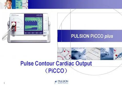
血流动力学监测 2011.11.30 血流动力学 ← 研究血液在心血管系统中流动的一系列物理学问题,即流量、阻力、压力之间的关系 ← 依据物理学定律,结合生理学和病理生理学的概念,对循环中血液运动的规律进行定量的、动态的、连续的测量分析,用于了解病情、指导治疗 ← 随着对疾病理解的深入和治疗要求的提高,临床上需要更多的参数来精确的反映病情的变化 ← 重症患者的治疗离开了监测会变的盲目;而监测方法离开了对治疗的反馈指导将变得无用 血流动力学监测的常规内容 ← 体循环: 心率、血压、CVP、CO、SVR← 肺循环: PAP、PAWP、PVR← 氧动力学参数: 氧输送(DO2)、氧消耗(VO2) ← 氧代谢参数: 血乳酸、SaO2、SvO2、ScvO2临床血流动力学监测 ← 容量评估及容量反应性 ← 细化体循环血压监测及指导治疗 ← 体循环氧动力学监测 ← 微循环监测 ← 线粒体功能的监测 临床血流动力学监测的核心内容 ← 评价体循环:容量复苏和药物治疗效果 ← 监测、评估微循环:组织灌注与氧代谢状况 容量评估及容量反应性 ← 容量治疗是重症患者治疗的基础措施,通常在临床治疗的最初阶段就已经开始 ← 合理的容量治疗取决于对患者容量状态的评估 ← 容量评估是临床治疗的基石,是血流动力学监测的关键 容量评估的指标 ← 静态前负荷指标压力负荷指标---CVP、PAWP心脏容积负荷指标---RVEDVI、GEDVI、ITBVI← 心肺相互作用相关的动态前负荷指标---SVV、SPV、PPV ← 容量负荷试验← 被动抬腿试验静态压力负荷指标----CVP、PAWP← 根据心室压力-容积曲线,由心腔压力间接反应前负荷← CVP近似右房压,PAWP反映左心舒张末压,是目前最常用的容量评估指标← 但其评估容量的临床价值存在争议心室顺应性正常 心室顺应性下降 心室顺应性增强 静态压力负荷指标----CVP、PAWP ← 压力负荷受到测量、胸腔内压、心率、心肌顺应性等多种因素影响,对前负荷的评估上有局限性← 静态或基础CVP和PAWP难以准确预测容量反应性← 将CVP8 -12mmHg、PAWP12 -15mmHg作为严重感染和感染性休克早期治疗的液体复苏目标,尚缺乏大规模临床试验证实,存在争议← CVP的价值体现在动态的变化和观察中,而不是仅仅某一孤立的数值心脏容积负荷指标 ← RVEDVI、GEDVI、ITBVI在压力变化过程中保持相对独立,不受胸腔内压或腹腔内压变化的影响← 能更准确的反应心脏容量负荷← 临床可通过PiCCO经肺热稀释技术测量得到 多个研究表明RVEDVI、GEDVI、ITBVI数值在正常范围低限时数值越低,液体反应性越好;数值越高,则液体反应性越差;中间数值不能预测液体反应性 心肺相互作用相关的动态前负荷指标← SVV、SPV、PPV是动态前负荷指标← SVV可以通过PiCCO或NICOM技术动态监测获得← 更准确的反应心室SV的变化← 机械通气时动脉压的波形和压力值随吸气、呼气相应发生升高、降低的周期性改变;血容量不足时,这种变化尤为显著← 机械通气时SV的变化幅度大,提示左、右心室均处于心功能曲线的上升支,此时容量反应性好;反之,提示至少一个心室处于心功能曲线的平台支,容量反应性差← 大量研究证实SVV、PPV、SPV预测容量反应的敏感性和特异性均明显优于静态前负荷← SVV、PPV、SPV是目前容量评估的重点 机械通气患者SVV正常值<10-15%SVV、PPV、SPV的临床使用受下列条件限制:容量控制通气潮气量恒定(8 -12ml/kg)窦性心律、无心律失常 对于非机械通气或存在心律失常的患者 如何评估容量? 容量负荷试验或被动抬腿试验Frank-Starling定律 ← 只有在左、右心室均处于心功能曲线上升支时,增加心脏前负荷才能显著提高心排量,即容量反应性好 ← 心室处于心功能曲线平台支时,即使增加心脏前负荷也难以进一步增加心排量,即容量反应性差,且可导致肺水肿等容量过度的危害 ← A:收缩力正常← B:收缩力增加← C:收缩力下降容量反应性 ← 目前无法评估机体的绝对容量值,主要通过容量治疗后机体反应,间接评估容量的需求← 容量反应性好是容量治疗的基本前提← 根据Frank-Starling定律,容量治疗后CO或SV较前增加≥12-15%,被认为是容量治疗有效容量负荷试验 ← 方法:在30分钟内输入晶体液500-1000ml或胶体液300-500ml,判断容量反应性及耐受性,从而决定是否继续容量治疗← 可通过监测CVP的动态变化,遵循“2-5”法则指导容量负荷试验← 容量负荷试验特点:要求加快输液速度! 被动抬腿试验(PLRT) ← PLRT相当于自体模拟的容量负荷试验,但受自身神经系统的调节,作用一般维持10分钟左右← 对于前负荷有反应的患者,通常在30-90秒内能见到最大反应,SV增加可达到10% -15%← 如果PLRT能够引起SV增加明显超过10%,那么容量负荷治疗可引起SV增加明显超过15%PLRTPLRT1. 患者位于半坐位(头抬高呈45度)或仰卧位2. 观察T1时间SV的数值3. 同时放平头部和/或升高脚的位置(脚抬高呈45度)4. 等待1分钟5. 观察T2时间SV的数值6. SV%增加>10-15%=前负荷有反应7. SV%增加<10-15%=前负荷无反应8. 必要时可重复上述操作← 可食道心脏超声同步监测PLRT期间主动脉流速的变化来预测容量反应性← PLRT后主动脉流速增加≥10-13%,预测容量治疗有反应,敏感性和特异性均大于80%← 近年PLRT的趋势,儿童可经胸超声获得主动脉流速的变化、成人经外周动脉流速来预测容量反应性 容量挑衅 对于非机械通气或存在心律失常的患儿,没有CVP和超声,如何评估容量反应? ← 容量负荷试验以20ml/kg晶体液在30分钟内输入← 或PLRT← 评估容量治疗后CO或SV较前是否增加≥12 -15% ← 是,前负荷有反应,可继续容量挑衅← 否,前负荷无反应,停止输液 体循环血压监测 ← MAP=舒张压+1/3脉压差MAP=CO*SVR=SV*HR*SVR← MAP是2001、2005版EGDT的主要治疗目标← 在NICOM或PiCCO指导下,动态监测SV和SVR有助于指导容量复苏,合理使用正性肌力药物、血管活性药物体循环氧动力学监测 ← 氧供(DO2)← 氧耗(VO2)← 氧债DO2← 氧供是每分钟内转运供应到组织的氧量,由血氧含量和心排量组成 ← 合适的氧供依赖于有效的肺气体交换、血红蛋白水平、足够的血氧饱和度和心排量 DO2------呼吸循环殊途同归← DaO2=[ (CO)×动脉氧含量(CaO2)] ← CO=SV×HR← CaO2=(1.38×Hgb×SaO2)+(0.0031×PaO2)← DaO2=SV×HR×[(1.38×Hgb×SaO2)+(0.0031×PaO2)]VO2← 氧耗是指组织所消耗的氧量,例如系统的气体交换 ← 此参数不能直接测得,可以通过动脉和静脉的氧供差值计算得出 ← VO2=DaO2-DvO2← VO2=CO×(CaO2-CvO2)×10← VO2=CO×Hgb×13.8×(SaO2-SvO2) ← VO2=5×15×13.8×(0.99-0.75)← 正常值=200-250ml O2/minVO2/DO2的关系← 正常情况下氧供大约为氧耗的四倍,所以氧需求量并不依赖于氧供,即曲线上的氧供非依赖区;此时如果氧供减少,细胞可以摄取更多的氧以维持氧耗的正常水平 ← 一旦这种代偿机制被耗竭,氧耗量就开始依赖于氧供,这段曲线被称为氧供依赖区 氧债 ← 当氧供不足以满足机体的需求时,则出现氧债 ← 一旦氧债出现,必须提供额外的氧供以偿还氧的欠缺 ← 氧需>氧耗=氧债 ← 影响氧债积蓄的因素: 氧供减少 细胞氧摄取减少 氧需求增加 微循环监测 ← 微循环障碍---严重全身性感染的早期事件 ← 微循环障碍意味着随之而来的细胞氧摄取障碍和微循环窘迫 微循环监测 ← SvO2/ScvO2← 血乳酸← Pcv-aCO2← 侧流暗视野视频显微镜技术(SDF)SvO2← VO2=C(a-v)O2×CO×10← 若SaO2=1.0 SvO2=1-[VO2/(CO×10×CaO2)] ← SvO2与氧供、氧耗有关SvO2与容量复苏← SvO2>65%、ScvO2>70%是2001、2005版EGDT 的治疗目标← 2009年哈佛医学院牵头的急诊医学休克协作组研究结果表明,SvO2<70%或>90%均导致死亡率增加,以SvO2达标或过高作为复苏目标存在片面性← SvO2异常升高提示组织氧利用障碍,此时需要观察微循环功能以及线粒体功能← SaO2↓← SvO2↓← CaO2-CvO2 —← SaO2—← SvO2↓← CaO2-CvO2↑← SaO2↓← SvO2↓← CaO2-CvO2↑← SaO2↑← SvO2—/↑← CaO2-CvO2—← SaO2—← SvO2↑← CaO2-CvO2↓← 肺氧合功能障碍 ← 周围组织循环不良 ← 组织代谢增加 ← 肺氧合功能下降伴心功能不全 (机械通气对循环的抑制) ← 吸氧或MV使肺氧合功能改善 ← 组织氧耗量降低(低温、镇静、肌松) ← 组织摄氧功能下降 (败血症、氰化物中毒、硝普钠应用) ← 肺外分流 不能单纯将高SvO2水平作为容量复苏的目标 乳 酸 ← 血乳酸是评价危重症严重程度及预后的指标← 血乳酸持续升高与APACHEII密切相关,感染性休克血乳酸>4mmol/L,病死率达80%← 目前多采用乳酸清除率和高乳酸(>2mmol/L)时间来作为评估指标 血乳酸水平与组织灌注、细胞缺氧,以及肝脏糖异生能力有关 Pcv-aCO2← 理论上,组织缺氧状态下组织PO2将下降,组织PCO2将升高,但实际并非如此← 内毒素血症组织PO2可能并不低---细胞病性缺氧← 低氧性缺氧时,组织PCO2没有升高;仅在缺血性缺氧时组织PCO2才明显升高← PCO2的上升与组织的灌注不足密切相关Pcv-aCO2← 微循环血流灌注不足即休克存在时,组织PO2将降低,组织PCO2将升高,反映的本质是组织局部DO2减少和缺氧代谢增加← 更高的组织PO2和更低的组织PCO2可能才是休克复苏的理想目标。
无创血流动力学参数心输出量(cardiac output,CO)、心脏指数(cardiac index,CI)是评价心功能及血流灌注的诊断指标,是机体功能发生重大变化时的早期报警。
每搏输出量(stroke volume,SV)的变化是机体血流量和心肌收缩发生变化的早期信号。
加速指数(acceleration index,ACI)、CI是评价心脏收缩功能的指标。
外周血管阻力(systemic vascular resistance ,SVR)、外周血管阻力指数(systemic vascular resistance index,SVRI)是反映心脏后负荷的参数,与外周阻力增加呈正相关,胸腔积液量(Thoracic fluid content,TFC)反映心脏前负荷。
血浆N端脑利钠肽(NT-ProBNP)是心室肌细胞合成和分泌的一种肽类物质,也被认为是一种心脏神经激素,是一种含32个氨基酸的多肽类神经激素,NT-ProBNP主要由心室肌细胞合成,当心室容积负荷和压力负荷增加时可刺激NT-ProBNP的分泌,引起排钠、利尿、扩张血管和抑制肾素--血管紧张素--醛固酮系统的效应,并且可抑制促肾上腺皮质激素的释放及交感神经的过度反应,参与调节血压、血容量和盐平衡,有排钠、利尿、扩血管等作用,它的血浆含量与心室的压力、呼吸困难的程度、神经激素调节系统的状况呈正比,NT-ProBNP 是左室收缩功能不全的最强的具有特异性的标志物,可以作为早期诊断心力衰竭的判断指标,2003年美国临床生化学会(NACB Guidelines)即把NT-ProBNP 作为早期检测CHF的标志物。
有研究发现,TFC与NT-ProBNP明显相关,收缩时间比率(Systolic Time Ratio,STR)反映心肌收缩力,STR高低与心功能恶化的严重程度有关;另有研究表明STR的变化与心脏超声射血分数值相关系数为0.85。
2012年欧洲心脏病协会(ESC)强调N末端前B型利钠肽(NT-proBNP)可用于可疑心衰患者的诊断和鉴别诊断,并强调这一生物学标志物的诊断和鉴别诊断价值,对于有症状的可疑心衰患者其阴性预测值和阳性预测值均很高,临床应用价值很高,推荐将NT-ProBNP与X线、超声心动图影像学及临床表现等结合诊断心衰并将其作为心衰的排除试验序,甚至在心衰的诊断流程中推荐先采用生物学标志物NT-ProBNP检测,而将超声心动图检查用于已确诊的心衰患者,以确定基础心血管疾病的病因、心脏损害的程度和评价心功能(如左心室射血分数)等,2013年美国心脏病学院基金会/美国心脏协会(ACCF/AHA;美国指南) 也更多的描述了这个指标在临床上的诊断意义以及对心衰严重程度和治疗效果的评价价值。
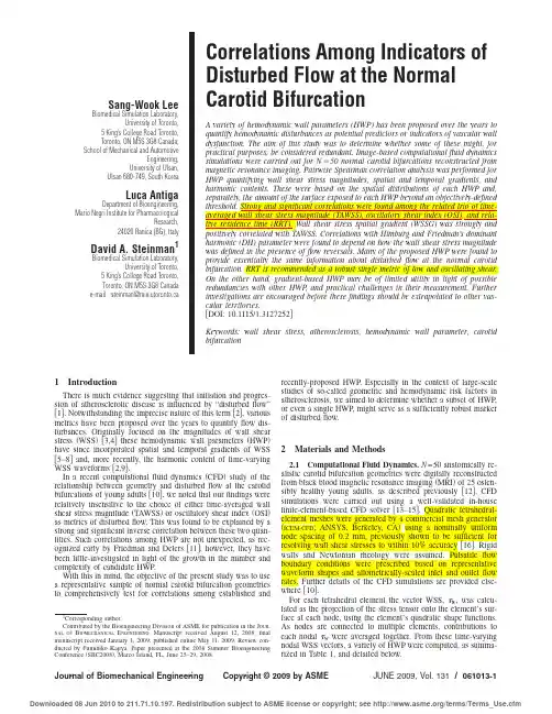
Sang-Wook Lee Biomedical Simulation Laboratory,University of Toronto,5King’s College Road Toronto,Toronto,ON M5S3G8Canada;School of Mechanical and AutomotiveEngineering,University of Ulsan,Ulsan680-749,South KoreaLuca AntigaDepartment of Bioengineering, Mario Negri Institute for PharmacologicalResearch,24020Ranica(BG),Italy David A.Steinman1Biomedical Simulation Laboratory,University of Toronto,5King’s College Road Toronto,Toronto,ON M5S3G8Canada e-mail:steinman@mie.utoronto.ca Correlations Among Indicators of Disturbed Flow at the Normal Carotid BifurcationA variety of hemodynamic wall parameters(HWP)has been proposed over the years to quantify hemodynamic disturbances as potential predictors or indicators of vascular wall dysfunction.The aim of this study was to determine whether some of these might,for practical purposes,be considered redundant.Image-based computationalfluid dynamics simulations were carried out for Nϭ50normal carotid bifurcations reconstructed from magnetic resonance imaging.Pairwise Spearman correlation analysis was performed for HWP quantifying wall shear stress magnitudes,spatial and temporal gradients,and harmonic contents.These were based on the spatial distributions of each HWP and,harmonic(DH)parameter were found to depend on how the wall shear stress magnitude was defined in the presence offlow reversals.Many of the proposed HWP were found to provide essentially the same information about disturbedflow at the normal carotid bifurcation.RRT is recommended as a robust single metric of low and oscillating shear. On the other hand,gradient-based HWP may be of limited utility in light of possible redundancies with other HWP,and practical challenges in their measurement.Further investigations are encouraged before thesefindings should be extrapolated to other vas-cular territories.͓DOI:10.1115/1.3127252͔Keywords:wall shear stress,atherosclerosis,hemodynamic wall parameter,carotid bifurcation1IntroductionThere is much evidence suggesting that initiation and progres-sion of atherosclerotic disease is influenced by“disturbedflow”͓1͔.Notwithstanding the imprecise nature of this term͓2͔,variousmetrics have been proposed over the years to quantifyflow dis-turbances.Originally focused on the magnitudes of wall shear stress͑WSS͓͒3,4͔these hemodynamic wall parameters͑HWP͒have since incorporated spatial and temporal gradients of WSS ͓5–8͔and,more recently,the harmonic content of time-varying WSS waveforms͓2,9͔.In a recent computationalfluid dynamics͑CFD͒study of the relationship between geometry and disturbedflow at the carotid bifurcations of young adults͓10͔,we noted that ourfindings were relatively insensitive to the choice of either time-averaged wall shear stress magnitude͑TAWSS͒or oscillatory shear index͑OSI͒as metrics of disturbedflow.This was found to be explained by a strong and significant inverse correlation between these two quan-tities.Such correlations among HWP are not unexpected,as rec-ognized early by Friedman and Deters͓11͔;however,they have been little-investigated in light of the growth in the number and complexity of candidate HWP.With this in mind,the objective of the present study was to use a representative sample of normal carotid bifurcation geometries to comprehensively test for correlations among established and recently-proposed HWP.Especially in the context of large-scalestudies of so-called geometric and hemodynamic risk factors inatherosclerosis,we aimed to determine whether a subset of HWP,or even a single HWP,might serve as a sufficiently robust markerof disturbedflow.2Materials and Methods2.1Computational Fluid Dynamics.N=50anatomically re-alistic carotid bifurcation geometries were digitally reconstructedfrom black blood magnetic resonance imaging͑MRI͒of25osten-sibly healthy young adults,as described previously͓12͔.CFDsimulations were carried out using a well-validated in-housefinite-element-based CFD solver͓13–15͔.Quadratic tetrahedral-element meshes were generated by a commercial mesh generator ͑ICEM-CFD;ANSYS,Berkeley,CA͒using a nominally uniform node spacing of0.2mm,previously shown to be sufficient forresolving wall shear stresses to within10%accuracy͓16͔.Rigidwalls and Newtonian rheology were assumed.Pulsatileflowboundary conditions were prescribed based on representativewaveform shapes and allometrically-scaled inlet and outletflowrates.Further details of the CFD simulations are provided else-where͓10͔.For each tetrahedral element the vector WSS,w,was calcu-lated as the projection of the stress tensor onto the element’s sur-face at each node,using the element’s quadratic shape functions. As nodes are connected to multiple elements,contributions to each nodalw were averaged together.From these time-varying nodal WSS vectors,a variety of HWP were computed,as summa-rized in Table1,and detailed below.1Corresponding author.Contributed by the Bioengineering Division of ASME for publication in the J OUR-NAL OF B IOMECHANICAL E NGINEERING.Manuscript received August12,2008;finalmanuscript received January1,2009;published online May11,2009.Review con-ducted by Fumihiko Kajiya.Paper presented at the2008Summer Bioengineering Conference͑SBC2008͒,Marco Island,FL,June25–29,2008.2.2Magnitude-Based HWP.Time-averaged wall shear stress was calculated by integrating each nodal WSS magnitude over the cardiac cycle.For each CFD model,the nodal TAWSS were normalized by the fully-developed ͑i.e.,Poiseuille ͒value,based on the model’s imposed cycle-averaged flow rate,the as-sumed viscosity,and the mean diameter ofthe model’s commoncarotid artery ͑CCA ͒at a location three radii upstream of the bifurcation ͑i.e.,CCA3,as defined in Ref.͓10͔͒.Oscillatory shear index,a dimensionless metric of changes in the WSS direction,originally introduced by Ku et al.͓6͔,was malized with respect to its fully-developed value at CCA3.2.3Gradient-Based HWP.Originally proposed by Lei et al.͓19͔,the wall shear stress spatial gradient ͑WSSG ͒may be con-sidered a marker of endothelial cell tension.As shown in Table 1,it is calculated from the WSS gradient tensor components parallel and perpendicular to the time-averaged WSS vector ͑m and n ,respectively ͒.Here the WSS gradients were calculated directly from the velocities of each element,taking advantage of their quadratic shape functions.As with WSS itself,elemental contri-butions to nodal WSSG values were averaged together.Since the WSSG of fully-developed flow in a straight uniform pipe is zero,here it is normalized by the fully-developed TAWSS divided by the mean diameter at CCA3.Subsequently,Longest and Kleinstreuer ͓20͔proposed the WSS angle gradient ͑WSSAG ͒to highlight regions exposed to large changes in WSS direction,irrespective of magnitude.As indicated by the formula in Table 1,this was done by calculating,for each element’s node ͑index j ͒,its direction relative to some reference WSS vector ͑index i ͒,here chosen to be that at the element’s centroid.The WSS temporal gradient ͑WSST ͒,originally suggested by Ojha ͓7͔as a factor in distal anastomotic intimal hyperplasia,is simply the maximum absolute rate of change in WSS magnitude over the cardiac cycle.Here it is normalized to WSST at location CCA3,determined from Womersley’s solution of fully-developed pulsatile flow based on the CCA3diameter,the heart rate,and the imposed flow rate Fourier coefficients.2.4Harmonic-Based HWP.Recently,Himburg and Fried-man ͓2͔suggested the harmonic content of the WSS waveform as a possible metric of disturbed flow,subsequently linking this to the frequency-dependent responses of endothelial cells ͓21͔.Fol-lowing those authors,the time-varying WSS magnitude at each node was Fourier-decomposed,with the dominant harmonic ͑DH ͒simply defined as the harmonic with the highest amplitude.Around the same time,Gelfand et al.͓9͔defined the harmonic index ͑HI ͒as the relative fraction of the harmonic amplitude spec-trum arising from the pulsatile flow components.Table 1Definitions of hemodynamic wall parameters …HWP …2.5Data Analysis.Correlations among the various HWP were evaluated in two ways:locally,whereby spatial distributionsof HWP were compared;and globally,whereby overall“burdens”of disturbedflow were compared.Local correlations were tested byfirst discretizing each model’ssurface into afinite number of contiguous patches,within each ofwhich the respective HWP was averaged͑for the ordinal DH,themedian was used͒.This amounted to mapping each distribution ofHWP onto an objective template plane,fixed with respect to abifurcation-specific coordinate system͓22͔.Remembering thatmodel dimensions have previously been normalized with respectto their respective CCA3radius,patches were nominally0.5unitsin length along the direction of the vessel axis,with12patchesdistributed circumferentially at each axial level.To facilitate pool-ing of patches from all cases,and in light of differences in eachCFD model’s relative length,only those patch locations presentfor all CFD models were included,resulting in288patches permodel.Although absolute patch sizes may have varied betweenand within models,this mapping procedure ensured that all sur-faces were spatially discretized in a consistent way͓22͔.Global comparisons were made by calculating,for each CFDmodel,the fraction of its surface area exposed to“abnormal”val-ues of a particular HWP.As detailed in Ref.͓10͔,“abnormal”wasdefined,for each HWP,as the upper quintile͑for TAWSS,thelower quintile͒of the HWP data pooled from all CFD models,thus providing an objective threshold between normal and abnor-mal.To ensure a consistent spatial extent across all cases,thesurfaces were clipped at planes three andfive maximally inscribedsphere radii along the common and internal carotid arteries ͑CCA3and ICA5,respectively͓10͔͒.Then,for each case,the area of the surface experiencing HWP above͑for TAWSS,below͒thethreshold was calculated.To factor out the influence of vesselsize—for the same shape,a larger vessel will experience a largerarea of disturbedflow—this absolute surface area was divided bythe total͑clipped͒surface area.In this way,for each HWP,eachCFD model was assigned a single value characterizing how muchof its surface was exposed to disturbedflow.For both local and global comparisons,a Spearman rank corre-lation coefficient͑r͒and significance͑p-value͒were computed for each of the28unique pairs of HWP using PRISM version4͑GraphPad Software,San Diego,CA͒.Correlations having p Ͻ0.05were deemed strong for͉r͉Ͼ0.8,weak for͉r͉Ͻ0.5,and moderate in between.Spearman correlation analysis was chosen in part because HWP distributions are unlikely to be normal.Also, in assessing these correlations based on rank,we sought to iden-tify,in the local correlations,whether the sites of extrema for one HWP would be reflected in the sites of extrema for another HWP. Global correlations sought to identify whether the ranking of cases from low to high burden of“disturbedflow,”based on the threshold of a given HWP,would be the same as that obtained based on another HWP.3ResultsAs depicted in Fig.1for a representative case,disturbedflow based on WSS magnitude quantities͑TAWSS,OSI,and RRT͒was concentrated around the outer walls of the bifurcation,consistent with many previous observations.For gradient-based HWP ͑WSSG,WSSAG,and WSST͒elevated values were concentrated around the bifurcation apex and,to a lesser but more variable extent,around the external and internal carotid artery͑ECA and ICA͒branches.Distributions of harmonic HWP͑DH and HI͒were more distinctive:higher DH was concentrated away from the outer walls of the bifurcation,whereas elevated HI reflected the general locations,if not the specific spatial extents,of the magnitude-based HWP.Overall,these observations hint at the correlations among the patched HWP distributions,detailed in Table2and depicted graphically for selected HWP pairs in Fig.2.Strong correlations were seen between TAWSS and both RRT͑r=−0.99͒and WSSG ͑r=0.86͒,albeit for different reasons:regions of elevated RRT correlated well with those experiencing low TAWSS͑r=−0.99͒, whereas elevated WSSG correlated with elevated TAWSS͑r =0.86͒.Moderate inverse correlations were found between TAWSS and both OSI and HI͑r=−0.66and r=−0.72,respec-tively͒,whereas TAWSS was positively correlated with WSST ͑r=0.63͒.Although many of the correlations were weak,all were statistically significant.Of all HWP,only DH was neither stronglynor moderately correlated with any other HWP.It is also worthnoting that the correlations identified by pooling the cases werefairly consistent across the50cases analyzed individually,as evi-denced by the relatively narrow confidence intervals shown in thesame table.According to the global correlations summarized in Table3,TAWSS,OSI,or RRT would rank vessels in similar order fromlow to high burdens of disturbedflow,as indicated by the strongpositive global correlation coefficients.Conversely,if disturbedflow was defined as elevated WSSG,vessels would be ranked inreverse order to this,as indicated by the moderate negative corre-lations with TAWSS,OSI,and RRT.As with the local correla-tions,HI was moderately correlated with the trio of magnitude-based HWP,while DH was only weakly correlated with otherHWP.Overall,corresponding local and global correlations wereof similar strength.A notable exception was OSI versus WSSAG, for which the local correlation was moderate͑r=0.73͒,while the global correlation was weak͑r=0.05͒and not significant.Reasons for this are given in Sec.4.It is worth noting that the above results were found to be rela-tively insensitive to the choice of data analysis method.For ex-ample,the Spearman correlation analysis of the continuous distri-butions of HWP͑i.e.,the CFD nodal values prior to patching͒revealed correlations similar to those obtained after patching.Glo-bal correlations based on a90th percentile threshold for disturbedflow were similar to those reported here using the80th percentilethreshold,afinding consistent with Ref.͓10͔.Finally,in light ofthe concentrations of HWP extrema around the bifurcation region,we repeated the local correlation analysis using patches extendingaxially only halfway along each branch͑i.e.144patches permodel͒to exclude the distal parts of the branches.Again thetrends were the same,although some of the moderate correlationsactually increased in strength,such as TAWSS versus OSI͑from r=−0.66to r=−0.77͒and TAWSS versus WSST͑from r=0.62to r=0.75͒.The detailed results are omitted in the interest of space, and because they do not affect the implications and conclusions discussed below.4Discussion4.1Summary and Implications of Findings.This compre-hensive evaluation of correlations among HWP at the normal ca-rotid bifurcation clearly demonstrates that some of these param-eters may,for practical purposes,be considered redundant.By virtue of their definitions in Table1,correlations among WSS, OSI,and RRT were expected,although not necessarily at the strengths observed.While WSS and OSI were moderately corre-lated,Fig.1suggests the OSI captures apparentflow disturbances at the ECA branch.Notwithstanding whether these are significant in the context of atherosclerosis—plaques do tend to occur at the ICA—our results would suggest that RRT can replace WSS and OSI as a single marker of“low and oscillatory”shear.In fact,as noted earlier,RRT is,by definition,the inverse of the magnitude of the time-averaged WSS vector.This explains its near-perfect correlation with TAWSS,which,remember,is the time-average of the WSS magnitude.In other words,RRT is simply another type of time-averaged WSS,but inverted and with a more tangible connection to the biological mechanisms underlying atherosclero-sis͓18͔.To appreciate the practical implications of replacing TAWSS and OSI with RRT,consider our recent study in which exposure todisturbed flow was found to be significantly predicted by a com-bination of bifurcation area ratio and tortuosity ͓10͔.There,the findings were shown to be independent of the choice of TAWSS or OSI as the metric of disturbed flow.Here,repeating the multiple regressions using RRT above the 80th percentile as the criterion for disturbed flow,we found near-identical—if anything,slightly stronger—coefficients:R adj 2=0.341͑p =0.0001͒,tortuosity =−0.498͑p =0.0001͒,and AR1=0.459͑p =0.0007͒.In other words,exposure of the vessels to “disturbed flow”is the same,whether defined by extrema of TAWSS,OSI,or RRT.The strong positive local correlations ͑and consequent strong negative global correlations ͒between TAWSS and its spatial and temporal gradients likely reflect the fact that all of these quantities are highest around the apex of the bifurcation.As pointed out by Ojha ͓7͔,the use of WSS spatial gradients as risk indicators for intimal thickening is questionable in light of their concentration about the bifurcation apex,a region usually spared of plaques.As suggested recently by Goubergrits et al.͓23͔,regions elsewhere experiencing elevated WSSG may represent a consequence of ath-erosclerosis rather than a cause.Either way,for the normal carotid bifurcation at least,our findings would suggest that TAWSS could be used instead of WSSG,which is anyway more susceptible to measurement uncertainty ͓24,25͔,owing to its reliance on spatial gradients.A similar conclusion may be drawn from the moderate correla-tions between TAWSS and WSST,although it is worth remember-ing that in this study all CFD models were exposed to the same waveform shape .Intersubject variations in waveform shape are reported to be on the order of 10%͓26,27͔.Such variations in flow rate dynamics have been found to have a relatively minor influence on variations in the distributions of a variety of HWP,at least relative to the influence of uncertainty in the reconstructed geometry ͓25͔.Thus,it is reasonable to conclude that our findings are robust to our assumptions about waveform shape.It was also observed that the spatial distributions of OSI and WSSAG were moderately correlated ͑r =0.73͒,consistent with previous qualitative observations for carotid bifurcations ͓25͔and coronary arteries ͓23͔.As pointed out by Goubergrits et al.͓23͔,WSSAG may be thought of as an extension of OSI;however,being based on differential versus integrated quantities,WSSAG distributions tend to be noisier and more sensitive to uncertainty,something evident here and also in Ref.͓25͔.Nevertheless,for the representative case presented in Fig.1,this correlation is less obvious.Elevated values of WSSAG do coincide with the periph-ery of those regions exposed to elevated OSI;however,the core region of elevated OSI at the carotid bulb is characterized by low WSSAG and,as with the other gradient-based HWP,elevated WSSAG is concentrated at the bifurcation apex,a regiontypicallyFig.1HWP distributions for a representative case.Except for the ordinal DH,contour levels de-picted in each frame’s legend correspond to the 80th,85th,90th,and 95th percentile values based on the HWP distribution pooled over all cases.Note identification of CCA3and ICA5clip planes in the upper left …TAWSS …panel.spared of atherosclerosis.Moreover,the global correlation of these quantities was much weaker ͑r =0.05͒.This may be ex-plained in reference to the respective scatter plot in Fig.2,which clearly shows that the local ͑i.e.,patchwise ͒Spearman rank cor-relation was biased by the preponderance of patches having low OSI and WSSAG values.Focusing only on those patches having OSI Ͼ0.1,it can be seen that there is no obvious correlation with WSSAG.Because the global correlations focused only on those regions exposed to the upper quintile of HWP values,they better reflect the correlation,or lack thereof,of these extrema.Having said this,it is worth noting that,for most of the other pairwise comparisons,global and local correlation coefficients were in much closer agreement.Of all HWP,only DH was found to be essentially independent of the other HWP.This was somewhat surprising,since Himburg and Friedman ͓2͔,in introducing the use of WSS harmonics as metrics of disturbed flow,reported an inverse correlation between DH and TAWSS ͑Pearson r =−0.62͒.By way of explaining this,we note that their study was carried out on porcine iliac arteries,which are nominally straight vessels experiencing largely axial flows.On the other hand,flow at the carotid bifurcation is decid-edly nonaxial,and likely subject to more reverse flow.In such regions,rectification of the time-varying WSS vector—remember that DH was derived here from the WSS vector magnitude,per its original definition ͓28͔—could alter its harmonic content.To appreciate the impact of this,we recomputed DH and HI using instead the time-varying “axial”WSS,namely,the compo-nent of the instantaneous WSS vector projected onto a unit vector defined by the direction of its time-averaged value.In this way,flow reversals relative to the nominal axial direction are pre-Table 2Spearman rank correlation coefficients for pairwise local comparisons of the pooled HWP distributions …N =14,400patches total ….Shown in brackets are 95%confidence intervals,drawn from pairwise comparisons of the 50datasets individually …N =288patches each ….All correlations significant to p <0.001,except WSSAG versus DH,p =0.03.OSIRRT WSSG WSSAG WSST DH HI TAWSS Ϫ0.66͓Ϫ0.76,Ϫ0.53͔Ϫ0.99͓Ϫ0.99,Ϫ0.98͔0.86͓0.80,0.91͔Ϫ0.29͓Ϫ0.41,Ϫ0.16͔0.63͓0.46,0.79͔Ϫ0.33͓Ϫ0.45,Ϫ0.21͔Ϫ0.72͓Ϫ0.81,Ϫ0.60͔OSI 0.72͓0.59,0.82͔Ϫ0.38͓Ϫ0.62,Ϫ0.16͔0.73͓0.68,0.78͔Ϫ0.27͓Ϫ0.47,Ϫ0.04͔0.06͓Ϫ0.08,0.16͔0.53͓0.39,0.66͔RRT Ϫ0.81͓Ϫ0.88,Ϫ0.72͔0.38͓0.25,0.52͔Ϫ0.57͓Ϫ0.74,Ϫ0.41͔0.30͓0.19,0.43͔0.74͓0.65,0.82͔WSSG 0.09͓Ϫ0.11,0.26͔0.67͓0.52,0.82͔Ϫ0.31͓Ϫ0.47,Ϫ0.14͔Ϫ0.51͓Ϫ0.67,Ϫ0.26͔WSSAG 0.07͓Ϫ0.13,0.24͔Ϫ0.02͓Ϫ0.15,0.10͔0.45͓Ϫ0.32,Ϫ0.55͔WSST Ϫ0.14͓Ϫ0.26,Ϫ0.04͔Ϫ0.08͓Ϫ0.38,0.15͔DH0.27͓0.14,0.41͔Fig.2Scatter plots for selected pairwise comparisons of HWP .Note that the local …patched …data are plotted using a log-log scale to better depict the full dynamic range of data.served.As can be seen by comparing Fig.3to Fig.1,this had a marked effect on the spatial distributions of DH and HI.The rea-son for this is also given in Fig.3:rectification of the instanta-neous WSS served to break up the clear fifth harmonic oscillation of the time-varying axial WSS in favor of the lower frequencies.As summarized in Table 4,this served to strengthen the correla-tions between the harmonic and other HWP.Of note is the local correlation coefficient for TAWSS versus DH ͑r =−0.69͒,now close to that originally reported by Himburg and Friedman.Whether DH and HI should be defined based on magnitude or axial WSS cannot be answered by the present study.It is also not clear whether DH should be considered a monotonic HWP in light of possible limits to the temporal response of endothelial cells to shear ͓21͔.Nevertheless,our findings do bring to attention a heretofore-underappreciated issue in the harmonic analysis of WSS in the presence of strongly nonaxial flow.4.2Potential Limitations.This study has made the custom-ary assumptions of rigid walls,Newtonian rheology,and fully-developed inlet boundary conditions,previously shown to be of relatively minor influence on the distribution of WSS ͓16,29,30͔.The use of allometrically-scaled flow rates was recently shown to have little impact on the relative burdens of disturbed flow among the 50cases considered here ͓10͔;however,as noted earlier,theassumption of a constant waveform shape might have served to underestimate variations in WSST,as well as the harmonic HWP.An obvious limitation of this study is the relatively narrow scope of vascular configurations considered,namely,normal ca-rotid bifurcations.We do note,however,that recent work from Goubergrits et al.͓23͔similarly reported possible redundancies among gradient and magnitude-based HWP for the case of a nor-mal coronary artery.Huo et al.͓31͔also noted a significant power-law relationship between TAWSS and OSI on the outer walls of the common carotid and celiac arteries,based on a CFD model of flow along the length of the mouse aorta.While a power-law relationship is expected based on the definition of OSI,those au-thors did note a difference in the power-law coefficients derived from the carotid and celiac sites,an observation consistent with the branch-specific clustering of data points in the OSI versus TAWSS scatter plot in Fig.2.Those authors also noted a corre-spondence between elevated TAWSS and elevated WSSG,al-though no quantitative relationship was found.Nevertheless,we encourage further investigation before our findings should be ex-trapolated to other vascular territories.It is also important to appreciate that our study has made no attempt to prioritize any of these HWP in terms of their purportedTable 3Spearman rank correlation coefficients for each pair-wise global comparison of the relative surface area exposed to the HWP beyond its 80th percentile value …N =50cases ….OSIRRT WSSG WSSAG WSST DH HI TAWSS 0.80a0.97aϪ0.63a Ϫ0.16Ϫ0.250.040.68a OSI 0.88aϪ0.50a 0.05Ϫ0.260.040.66a RRT Ϫ0.63aϪ0.10Ϫ0.250.020.74a WSSG 0.58a0.54a Ϫ0.33b Ϫ0.27WSSAG 0.43cϪ0.240.20WSST Ϫ0.20Ϫ0.04DH0.01ap Ͻ0.05.bp Ͻ0.01.cp Ͻ0.001.Fig.3Distributions of DH and HI based on the axial WSS component rather than WSS magnitude,shown for same case depicted in Fig.1.The arrows indicate the site of the time-varying WSS waveforms and corresponding spectra shown to the right.Table 4Spearman rank correlation coefficients for local and global comparisons of DH and HI,as derived from the time-varying axial WSS rather than the WSS magnitude.Local GlobalDHHI DH HI TAWSS Ϫ0.69a Ϫ0.77a 0.76a 0.83a OSI 0.55a 0.65a 0.78a 0.89a RRT 0.70a 0.81a 0.78a 0.89a WSSG Ϫ0.58a Ϫ0.54a Ϫ0.54b Ϫ0.46a WSSAG 0.31a 0.51a Ϫ0.180.12WSST Ϫ0.36aϪ0.14a Ϫ0.34cϪ0.15DH0.63a0.64aap Ͻ0.05.bp Ͻ0.01.cp Ͻ0.001.links to the underlying biological mechanisms.Thus,some of the HWP we regard here as redundant might be shown to have closer mechanistic links in studies of individual biological responses to the local hemodynamic environment.Rather,we suggest that our findings are most applicable to large-scale studies of hemody-namic factors in atherosclerosis,which are more concerned with quantifying overall burdens or identifying patterns of localization of disturbedflow,whatever this vague term may prove to mean precisely.5ConclusionsFor the normal carotid bifurcation at least,many of the pur-ported indicators of disturbedflow are significantly correlated. Based on thesefindings we recommend the use of relative resi-dence time͑RRT͒as a robust single metric of low and oscillatory shear.In light of possible redundancies,any perceived benefits of gradient-based HWP are likely outweighed by practical challenges with their measurement.Dominant harmonic͑DH͒is a promising new HWP,but issues related to its definition in nonaxialflow need to be resolved.AcknowledgmentThe authors thank Dr.Mort Friedman for helpful discussions. The authors also thank the anonymous reviewers for their valu-able suggestions.DAS acknowledges the support of Grant No. MOP-62934from the Canadian Institutes of Health Research. SWL and DAS were supported by,respectively,a postdoctoral fellowship and a career investigator award from the Heart and Stroke Foundation.References͓1͔Chien,S.,2008,“Effects of Disturbed Flow on Endothelial Cells,”Ann.Biomed.Eng.,36͑4͒,pp.554–562.͓2͔Himburg,H.A.,and Friedman,M.H.,2006,“Correspondence of Low Mean Shear and High Harmonic Content in the Porcine Iliac Arteries,”ASME J.Biomech.Eng.,128͑6͒,pp.852–856.͓3͔Caro,C.G.,Fitz-Gerald,J.M.,and Schroter,R.C.,1971,“Atheroma and Arterial Wall Shear.Observation,Correlation and Proposal of a Shear Depen-dent Mass Transfer Mechanism for Atherogenesis,”Proc.R.Soc.London,Ser.B,177͑1046͒,pp.109–159.͓4͔Fry,D.L.,1968,“Acute Vascular Endothelial Changes Associated With In-creased Blood Velocity Gradients,”Circ.Res.,22͑2͒,pp.165–197.͓5͔Friedman,M.H.,and Ehrlich,L.W.,1975,“Effect of Spatial Variations in Shear on Diffusion at the Wall of an Arterial Branch,”Circ.Res.,37͑4͒,pp.446–454.͓6͔Ku,D.N.,Giddens,D.P.,Zarins,C.K.,and Glagov,S.,1985,“Pulsatile Flow and Atherosclerosis in the Human Carotid Bifurcation.Positive Correlation Between Plaque Location and Low Oscillating Shear Stress,”Arteriosclerosis ͑Dallas͒,5͑3͒,pp.293–302.͓7͔Ojha,M.,1994,“Wall Shear Stress Temporal Gradient and Anastomotic Inti-mal Hyperplasia,”Circ.Res.,74͑6͒,pp.1227–1231.͓8͔Hyun,S.,Kleinstreuer,C.,and Archie,J.P.,Jr.,2000,“Hemodynamics Analy-ses of Arterial Expansions With Implications to Thrombosis and Restenosis,”Med.Eng.Phys.,22͑1͒,pp.13–27.͓9͔Gelfand,B.D.,Epstein,F.H.,and Blackman,B.R.,2006,“Spatial and Spec-tral1heterogeneity of Time-Varying Shear Stress Profiles in the Carotid Bifur-cation by Phase-Contrast MRI,”J.Magn.Reson Imaging,24͑6͒,pp.1386–1392.͓10͔Lee,S.W.,Antiga,L.,Spence,J.D.,and Steinman,D.A.,2008,“Geometry of the Carotid Bifurcation Predicts Its Exposure to Disturbed Flow,”Stroke, 39͑8͒,pp.2341–2347.͓11͔Friedman,M.H.,and Deters,O.J.,1987,“Correlation Among Shear Rate Measures in Vascular Flows,”ASME J.Biomech.Eng.,109͑1͒,pp.25–26.͓12͔Thomas,J.B.,Antiga,L.,Che,S.L.,Milner,J.S.,Hangan-Steinman,D.A., Spence,J.D.,Rutt,B.K.,and Steinman,D.A.,2005,“Variation in the Carotid Bifurcation Geometry of Young Versus Older Adults:Implications for Geo-metric Risk of Atherosclerosis,”Stroke,36͑11͒,pp.2450–2456.͓13͔Ethier,C.R.,Steinman,D.A.,and Ojha,M.,1999,“Comparisons Between Computational Hemodynamics,Photochromic Dye Flow Visualization and Magnetic Resonance Velocimetry,”The Haemodynamics of Arterial Organs—Comparison of Computational Predictions With In Vivo and In Vitro Data,X.Y.Xu,and M.W.Collins,eds.,WIT,Southampton,UK,pp.131–183.͓14͔Minev,P.D.,and Ethier,C.R.,1999,“A Characteristic/Finite Element Algo-rithm for the3D Navier–Stokes Equations Using Unstructured Grids,”Com-put.Methods Appl.Mech.Eng.,178,pp.39–50.͓15͔Ethier,C.R.,Prakash,S.,Steinman,D.A.,Leask,R.L.,Couch,G.G.,and Ojha,M.,2000,“Steady Flow Separation Patterns in a45Degree Junction,”J.Fluid Mech.,411,pp.1–38.͓16͔Moyle,K.R.,Antiga,L.,and Steinman,D.A.,2006,“Inlet Conditions for Image-Based CFD Models of the Carotid Bifurcation:Is It Reasonable to Assume Fully Developed Flow?,”ASME J.Biomech.Eng.,128͑3͒,pp.371–379.͓17͔He,X.,and Ku,D.N.,1996,“Pulsatile Flow in the Human Left Coronary Artery Bifurcation:Average Conditions,”ASME J.Biomech.Eng.,118͑1͒, pp.74–82.͓18͔Himburg,H.A.,Grzybowski,D.M.,Hazel,A.L.,LaMack,J.A.,Li,X.M., and Friedman,M.H.,2004,“Spatial Comparison Between Wall Shear Stress Measures and Porcine Arterial Endothelial Permeability,”Am.J.Physiol.Heart Circ.Physiol.,286͑5͒,pp.H1916–1922.͓19͔Lei,M.,Kleinstreuer,C.,and Truskey,G.A.,1996,“A Focal Stress Gradient-Dependent Mass Transfer Mechanism for Atherogenesis in Branching Arter-ies,”Med.Eng.Phys.,18͑4͒,pp.326–332.͓20͔Longest,P.W.,and Kleinstreuer,C.,2000,“Computational Haemodynamics Analysis and Comparison Study of Arterio-Venous Grafts,”J.Med.Eng.Tech-nol.,24͑3͒,pp.102–110.͓21͔Himburg,H.A.,Dowd,S.E.,and Friedman,M.H.,2007,“Frequency-Dependent Response of the Vascular Endothelium to Pulsatile Shear Stress,”Am.J.Physiol.Heart Circ.Physiol.,293͑1͒,pp.H645–H653.͓22͔Antiga,L.,and Steinman,D.A.,2004,“Robust and Objective Decomposition and Mapping of Bifurcating Vessels,”IEEE Trans.Med.Imaging,23͑6͒,pp.704–713.͓23͔Goubergrits,L.,Kertzscher,U.,Schoneberg,B.,Wellnhofer,E.,Petz,C.,and Hege,H.C.,2008,“CFD Analysis in an Anatomically Realistic Coronary Artery Model Based on Non-Invasive3D Imaging:Comparison of Magnetic Resonance Imaging With Computed Tomography,”Int.J.Card.Imaging, 24͑4͒,pp.411–421.͓24͔Glor,F.P.,Long,Q.,Hughes,A.D.,Augst,A.D.,Ariff,B.,Thom,S.A., Verdonck,P.R.,and Xu,X.Y.,2003,“Reproducibility Study of Magnetic Resonance Image-Based Computational Fluid Dynamics Prediction of Carotid Bifurcation Flow,”Ann.Biomed.Eng.,31͑2͒,pp.142–151.͓25͔Thomas,J.B.,Milner,J.S.,Rutt,B.K.,and Steinman,D.A.,2003,“Repro-ducibility of Image-Based Computational Fluid Dynamics Models of the Hu-man Carotid Bifurcation,”Ann.Biomed.Eng.,31͑2͒,pp.132–141.͓26͔Ford,M.D.,Alperin,N.,Lee,S.H.,Holdsworth,D.W.,and Steinman,D.A., 2005,“Characterization of V olumetric Flow Rate Waveforms in the Normal Internal Carotid and Vertebral Arteries,”Physiol.Meas,26͑4͒,pp.477–488.͓27͔Holdsworth,D.W.,Norley,C.J.,Frayne,R.,Steinman,D.A.,and Rutt,B.K., 1999,“Characterization of Common Carotid Artery Blood-Flow Waveforms in Normal Human Subjects,”Physiol.Meas,20͑3͒,pp.219–240.͓28͔Friedman,M.H.,2008,personal communication.͓29͔Lee,S.W.,and Steinman,D.A.,2007,“On the Relative Importance of Rhe-ology for Image-Based CFD Models of the Carotid Bifurcation,”ASME J.Biomech.Eng.,129͑2͒,pp.273–278.͓30͔Younis,H.F.,Kaazempur-Mofrad,M.R.,Chan,R.C.,Isasi,A.G.,Hinton,D.P.,Chau,A.H.,Kim,L.A.,and Kamm,R.D.,2004,“Hemodynamics and Wall Mechanics in Human Carotid Bifurcation and Its Consequences for Atherogenesis:Investigation of Inter-Individual Variation,”Biomech.Model.Mechanobiol.,3͑1͒,pp.17–32.͓31͔Huo,Y.,Guo,X.,and Kassab,G.S.,2008,“The Flow Field Along the Entire Length of Mouse Aorta and Primary Branches,”Ann.Biomed.Eng.,36͑5͒, pp.685–699.。

cbf血流动力学指标摘要:一、概念介绍1.cbf 血流动力学指标是什么2.cbf 血流动力学指标的作用二、cbf 血流动力学指标的计算方法1.如何计算cbf 血流动力学指标2.cbf 血流动力学指标的计算公式三、cbf 血流动力学指标的临床应用1.cbf 血流动力学指标在临床上的应用2.cbf 血流动力学指标与疾病的关系四、cbf 血流动力学指标的优缺点1.cbf 血流动力学指标的优点2.cbf 血流动力学指标的缺点五、结论1.cbf 血流动力学指标的重要性2.未来研究方向正文:cbf 血流动力学指标,全称为脑血流量(cerebral blood flow),是一种反映脑部血流情况的指标,对于了解脑部血液循环、诊断疾病以及评估治疗效果具有重要意义。
cbf 血流动力学指标的计算方法主要包括两种:一种是通过对脑部进行磁共振成像(MRI)或CT 扫描,通过测量局部脑组织的血容量(CBV)和平均传输时间(MTT),然后使用公式cbf = CBV × MTT 进行计算;另一种方法是通过放置脑血管传感器,直接测量脑部的血流量。
在临床应用方面,cbf 血流动力学指标被广泛应用于神经内科、神经外科、重症监护室等多个领域。
通过cbf 血流动力学指标的测量,可以了解患者的脑部血流情况,帮助医生诊断疾病,如脑缺血、脑出血、颅内感染等。
此外,cbf 血流动力学指标还可以用于评估治疗效果,如脑血管病变的药物治疗、介入治疗等。
然而,cbf 血流动力学指标也存在一定的局限性。
首先,由于测量方法的限制,cbf 血流动力学指标可能存在一定误差。
其次,cbf 血流动力学指标受到个体差异、年龄、性别等因素的影响,因此在应用时需要综合考虑。
总之,cbf 血流动力学指标是一种重要的临床参数,对于了解脑部血流情况、诊断和治疗疾病具有重要意义。
判断颈动脉狭窄的常规血流动力学指标颈动脉狭窄是一种常见的血管疾病,其主要表现为颈部血管内膜增厚和斑块形成,导致血管腔狭窄,从而影响到大脑的供血。
因此,判断颈动脉狭窄的程度和危险程度对于预防中风等并发症具有重要意义。
本文将介绍常规血流动力学指标在判断颈动脉狭窄方面的主要内容。
一、颈动脉超声检查颈动脉超声检查是目前最常用的诊断颈动脉狭窄的方法之一。
通过超声波探头在颈部皮肤上扫描,可以观察到颈动脉内径、血流速度和流量等参数,并根据这些参数来评估颈动脉是否存在狭窄。
其中,最常用的指标是速度比(velocity ratio),即测量收缩期峰值流速(peak systolic velocity)与远端正常段峰值流速之比。
一般认为,速度比大于2.0表示没有明显的狭窄;速度比在1.5-2.0之间表示轻度狭窄;速度比在1.0-1.5之间表示中度狭窄;速度比小于1.0表示重度狭窄或闭塞。
二、颈动脉血流量测定颈动脉血流量测定可以更加准确地评估颈动脉的狭窄程度和危险程度。
该方法需要使用多普勒超声仪,通过对颈动脉内径和血流速度的测量,计算出颈动脉的血流量。
一般认为,颈动脉血流量在50-70ml/min之间为正常范围,低于50ml/min表示轻度到中度狭窄,低于30ml/min则表示重度狭窄或闭塞。
三、颈动脉硬化指数颈动脉硬化指数(atherosclerosis index)是评估颈动脉硬化程度的一个指标。
它是由多普勒超声仪自动生成的一个计算公式,包括了收缩期峰值流速、舒张期峰值流速和平均流速等参数。
一般认为,颈动脉硬化指数越高,则表明颈动脉内壁越厚,斑块越多,狭窄程度越严重。
四、颈动脉弹性指数颈动脉弹性指数(carotid artery elasticity index)是评估颈动脉弹性的一个指标。
它是由多普勒超声仪测量颈动脉内径和收缩期峰值流速的变化率得出的。
一般认为,颈动脉弹性指数越低,则表明颈动脉硬度越高,狭窄程度越严重。
结合生理学重新定义无创血流动力学部分参数含义心排量:反映心脏射血功能的指标。
心输出量(CO):一侧心室每分钟的射血量,等于心率乘以每搏输出量。
成年人大概在5L、min,成年男性比女性稍高。
一个成年人安静状态下的心输出量称为静息输出量,小孩约为4L/min,一个80岁的老年人约为2L/min,在妊娠、情绪激动时可升高。
心脏指数(CI):因每个个体的身材不一,心输出量不足以反映患者的心脏泵血功能,故提出心脏指数。
心脏指数是指心输出量除以体表面积,具体值不详。
心搏量(SV):指单侧心室在一个心脏周期中的射血量,等于舒张末期与收缩末期的差值,均值为70ml。
心搏指数(SI):因舒张末期容积与收缩末期容积会有一定范围内的变化,引出百分比的概念,即心搏量与舒张末期容积的比值,EF=SV/舒张末期心室容积×100%。
EF值除以体表面积。
SI=SV/(舒张末期心室容积×体表面积)×100%。
心率变律性:正常成年人安静状态下心率可在一定范围内变化,约60-100次/分,小孩和老人其变异性可能更大,成年人因为性别、年龄及其他原因也存在不同程度的变化。
同一个个体也可出现节律的变化,称为心率变律性,主要还是指心脏节律的变化,包括节律不齐、节律过快、过慢,同时也受年龄、性别、婚姻状况、基础疾病、药物、环境等影响。
前负荷(主要是心脏收缩期末期的容积+射血期的容积即每搏量。
)胸液传导性(TFC):体液包括细胞内液(各种细胞内的液体)、细胞外液(组织间液、血浆、心包液、胸腔液)、皮肤表面是否干燥。
胸液传导性主要是指以上各种液体将其信号通过无创血流机系统转化为我们可识别的信息。
每搏变异率(SVV):每搏量可在一定范围内变化,其变化的频率也有所不同,具有个体差异性。
血管容积:在前负荷里面主要指体循环静脉系统和肺动脉内的血管容量。
后负荷每搏外周阻力(SSVRI):指一个心动周期中外周动脉的压力,多数时候以血压表示。
推荐不同孕期的脐动脉血流参数正常值: 脐动脉血流变化,反映血管阻力情况.⑴脐动脉收缩期峰值和舒张末期流速之比(S/D), S 代表收缩期峰值流速,反映 血流量,D 代表舒张末期流速,反映胎盘血管阻力.正常妊娠脐动脉血流S/D 值岁 孕周增大而逐渐降低,S/D 从早孕大于4,随着孕周增长可以降到小于3,甚至是2 以下.这表明胎盘逐渐成熟,胎盘内血管包括母体妊娠子宫血液循环那部分的动 脉/静脉逐渐增多.增粗,胎盘外周阻力下降.使脐动脉在舒张期时仍能维持足够 的血流一满足胎儿的雪供.⑵测量脐动脉血流S/D 值最佳测量位置是脐动脉与胎盘附着处,这里测出的值 要比靠近胎儿侧段的值低,所以不要随意的见到脐动脉就测出一个比值.越是靠 近胎盘侧越好.⑶脐动脉血流S/D 值增高常见于妊高症引起的胎盘功能不全.脐动脉扭曲.和母 亲糖尿病.(4)脐动脉血流S/D 值一般在孕32周以后 ........ 2.7加减0.5左右.孕周脐动脉血流S/D 值4.73(左右)4.284.144.073.863.823.763.653.593.483.423.313.193.143.08 35 2.9636 2.852.742.742.622.512.39超声医学》第四版资料 正常妊娠在第22孕周前,脐动脉血流频谱变化不大。
收缩期血流速度波形陡而 尖舒张期血流相对较低据国内外有关报道:脐动脉流速的A/B 值在第20孕周为3.9第30孕周前A/B 值下降较迅速以后下降较平稳至30孕周后下降至3.0以下20 21 22 23 24 25 26 27 28 29 30 31 32 33 37 38 39 40 41我们这里较多的测量脐动脉的S/D值对于>32孕周的测量,<3视为正常,孕足月的应<2.5测量的意义主要是看是否有胎儿宫内窘迫的情况脐动脉孕周PI RI21-24 1.08(+/-)0.22 0.64(+/-)0.0825-26 1.02(+/-)0.20 0.65(+/-)0.0627 1.00(+/-)0.20 0.63(+/-)0.0728 0.95(+/-)0.19 0.63(+/-)0.0729 1.00(+/-)0.23 0.63(+/-)0.0830 1.01(+/-)0.26 0.62(+/-)0.0731 1.02(+/-)0.26 0.64(+/-)0.0932 0.95(+/-)0.21 0.62(+/-)0.0833 0.93(+/-)0.19 0.60(+/-)0.0834 0.90(+/-)0.21 0.58(+/-)0.0935 0.85(+/-)0.16 0.57(+/-)0.0736 0.86(+/-)0.48 0.57(+/-)0.0737 0.86(+/-)0.16 0.57(+/-)0.0738 0.86(+/-)0.20 0.56(+/-)0.0839 0.84(+/-)0.15 0.56(+/-)0.0840 0.84(+/-)0.15 0.55(+/-)0.08脐动脉血流检测技术及其临床应用Fitzgerald和Drrmn在1997年首次成功的记录胎儿脐动脉血流信号fetal umbilicalartery tlow signal),这一■技术为了解胎儿-胎盘循环的血液动力学改变提供了一种简便、有效、可重复、无创伤的检测方法,对于高危妊娠的监测及围产儿结局的预测有重要作用,是其它产前检测方法所不能代替的。
推荐不同孕期的脐动脉血流参数正常值:脐动脉血流变化,反映血管阻力情况.(1)脐动脉收缩期峰值和舒张末期流速之比(S/D), S代表收缩期峰值流速,反映血流量,D代表舒张末期流速,反映胎盘血管阻力.正常妊娠脐动脉血流S/D值岁孕周增大而逐渐降低,S/D从早孕大于4,随着孕周增长可以降到小于3,甚至是2以下.这表明胎盘逐渐成熟,胎盘内血管包括母体妊娠子宫血液循环那部分的动脉/静脉逐渐增多.增粗,胎盘外周阻力下降.使脐动脉在舒张期时仍能维持足够的血流一满足胎儿的雪供.(2)测量脐动脉血流S/D值最佳测量位置是脐动脉与胎盘附着处,这里测出的值要比靠近胎儿侧段的值低,所以不要随意的见到脐动脉就测出一个比值.越是靠近胎盘侧越好.(3)脐动脉血流S/D值增高常见于妊高症引起的胎盘功能不全.脐动脉扭曲.和母亲糖尿病.(4)脐动脉血流S/D值一般在孕32周以后.....2.7加减0.5左右.孕周脐动脉血流S/D值20 4.73(左右)21 4.2822 4.1423 4.0724 3.8625 3.8226 3.7627 3.6528 3.5929 3.4830 3.4231 3.3132 3.1933 3.1434 3.0835 2.9636 2.8537 2.7438 2.7439 2.6240 2.5141 2.39超声医学》第四版资料正常妊娠在第22孕周前,脐动脉血流频谱变化不大。
收缩期血流速度波形陡而尖舒张期血流相对较低据国内外有关报道:脐动脉流速的A/B值在第20孕周为3.9第30孕周前A/B值下降较迅速以后下降较平稳至30孕周后下降至3.0以下我们这里较多的测量脐动脉的S/D值对于>32孕周的测量,<3视为正常,孕足月的应<2.5测量的意义主要是看是否有胎儿宫内窘迫的情况脐动脉孕周 PI RI21-24 1.08(+/-)0.22 0.64(+/-)0.0825-26 1.02(+/-)0.20 0.65(+/-)0.0627 1.00(+/-)0.20 0.63(+/-)0.0728 0.95(+/-)0.19 0.63(+/-)0.0729 1.00(+/-)0.23 0.63(+/-)0.0830 1.01(+/-)0.26 0.62(+/-)0.0731 1.02(+/-)0.26 0.64(+/-)0.0932 0.95(+/-)0.21 0.62(+/-)0.0833 0.93(+/-)0.19 0.60(+/-)0.0834 0.90(+/-)0.21 0.58(+/-)0.0935 0.85(+/-)0.16 0.57(+/-)0.0736 0.86(+/-)0.48 0.57(+/-)0.0737 0.86(+/-)0.16 0.57(+/-)0.0738 0.86(+/-)0.20 0.56(+/-)0.0839 0.84(+/-)0.15 0.56(+/-)0.0840 0.84(+/-)0.15 0.55(+/-)0.08脐动脉血流检测技术及其临床应用Fitzgerald和Drrmn在1997年首次成功的记录胎儿脐动脉血流信号(fetal umbilicalartery tlow signal),这一技术为了解胎儿-胎盘循环的血液动力学改变提供了一种简便、有效、可重复、无创伤的检测方法,对于高危妊娠的监测及围产儿结局的预测有重要作用,是其它产前检测方法所不能代替的。