文化距离原始数据 6-dimensions-for-website-2015-08-16

格式：xls
大小：34.50 KB
文档页数：8

下载文档原格式

Crouse-Hinds SERIES MEDC signalling and alarms PB

OverviewThese new and improved manual alarm call points have been designed for use in hazardous locations and harsh environmental conditions. The GRP enclosure is suitable for use onshore or offshore where light weight combined with a high level of corrosion resistance is required. The unit is now supplied with a lift flap that latches firmly in place.Features• ATEX certified • IECEx certified• UL certified for Haz locs • UL certified for Ord locs • TR CU certified• Chinese (CQST) certified • Brazilian (INMETRO) certified • CCOE certified• DNV type approval (IEC 60945)• SIL 2 certified •IP66 and IP67• Corrosion free GRP construction • Variety of colours available • Up to 9 terminals available • Optional LED – indicates that the unit has been operated• Earth continuity option for metal glands• 1 or 2 changeover switches • Captive cover screws • Lift flap as standard•Latching as standard. Self reset (momentary) availableMEDC signalling and alarmsPB manual call point rangeEx de, Ex ia, weatherproofAll specifications, dimensions, weights and tolerances are nominal (typical) and Eaton reserve the right to vary all data without prior notice.No liability is accepted for any consequence of use.EatonUnit B, Sutton Parkway Oddicroft Lane Sutton in Ashfield United Kingdom NG17 5FBT: +44 (0) 1623 444 /hac *******************© 2015 EatonAll Rights Reserved Printed in UK PublicationNo.DSMC0031/B November 2017Eaton is a registered trademark.All other trademarks are property of their respective owners.Please check here for latest version of the datasheetModelPBW PBUL PBE PBI CSA -40°C to +70°C-25°C to +55°C†-40°C to +70°C*-40°C to +70°C-30°C to +40°CEN60079-0, EN60079-1, EN60079-7, EN60079-31Ex de IIC T6 Gb, Ex tb IIIC T85ºC Db (switch only)Ex de mb IIC T6 Gb, Ex tb IIIC T85ºC Db (with LED)Ex de mb IIC T4 Gb, Ex tb IIIC T135ºC Db (with resistors & diodes)ATEX Ex iaCert no. Baseefa 03ATEX0084X. ATEX Approved Ex II 1GD Certified to: EN60079-0, EN60079-11Ex ia IIC T4 Ga , Ex ia IIIC T135ºC Da IECEx Ex iaCert. no. IECEx BAS 12.0093XCertified to: IEC 60079-0, IEC 60079-11Ex ia IIC T4 Ga, Ex ia IIIC T135ºC DaULListing no. E186629UL listed to Class 1, Div 2. Groups A,B,C & D UL listed for Ordinary Locations. Listing no. S8117CSA Cert. no. 79120-3. Class 1 groups A,B,C & DTR CU Ex ed1Ex d e IIC T6 Gb, Ex tb IIIC T85°C Db (switch only)1Ex d e mb IIC T6 Gb X, Ex tb IIIC T85°C Db X (with LED)T emperature * -35°C to + 70ºC with LED† -25°C to +50°C with resistors or LED fittedIngress protection IP66 & IP67Entries Up to 4 entries, M16 or M20 top and bottom (1/2” NPT available on UL ver-sion)T erminals 7 x 2.5mm 2 – standard9 x 2.5mm 2 optional – up to 60V onlyResistors Various configurations available on versions up to 24V and all ‘IS’ versions. (Minimum Resistor value 100ΩPBE, 470ΩPBI)Earth continuity Internal and external earth continuity is provided with an optional earth plate LED indicationA high intensity red LED can be fitted as an optional extra to indicate operation on versions up to 24V and all ‘IS’ versionsAs standard the LED is not provided with over current protection. The forward current (If) should be limited to 20mALabellingDuty label – worded to customers requirements. Riveted on Tag label – worded to customers requirements. Screwed on Switch ratings (1 or 2changeover switches fitted)Switch only 30Vdc 5A (resistive) or 3A (inductive) 30-50Vdc 1A (resistive or inductive) 250Vac 5A (resistive or inductive) LED 24Vdc 0.05A Resistor(s) 24Vdc 0.05ADSMC0031/B 11/17The following code is designed to help in selection of the correct unit. Build up the reference number by inserting the code for each component into the appropriate boxOrdering requirements。

跨文化交流-权利距离

Formation and definition of PDI 权力距离指数的来源和定义
Status 现状 Formation 形成、来源 Definition 定义 Please turn to our handouts 请同学们看材料
Status现状：Inequality in society
There is inequality everywhere, in any society. Some people are stronger, smarter, wealthier, or more powerful than some other people. But Physical and intellectual capacities, power, wealth, and status may or may not go together.
Children are expected and educated to be obedient to their parents. Independent behavior of child is not encouraged. Younger ones are always being taken care of by older ones and parents. Younger children are expected to yield to older ones. Authority continues to play a role in children’s life, even if they are adults.
Power is centralized as much as possible in a few hands. Subordinates expect to be told what to do. An ideal boss is a good father. Privileges and status symbols are expected and popular.

Website-httppyrx.scripps.edu

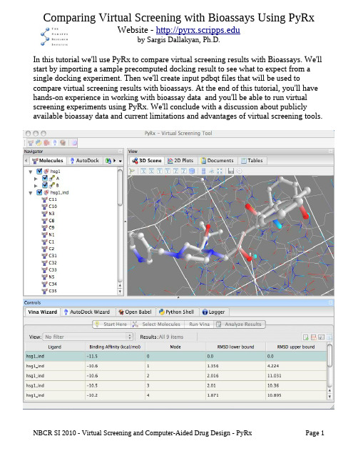
Comparing Virtual Screening with Bioassays Using PyRxWebsite - by Sargis Dallakyan, Ph.D.In this tutorial we'll use PyRx to compare virtual screening results with Bioassays. We'll start by importing a sample precomputed docking result to see what to expect from a single docking experiment. Then we'll create input pdbqt files that will be used to compare virtual screening results with bioassays. At the end of this tutorial, you'll have hands-on experience in working with bioassay data and you'll be able to run virtual screening experiments using PyRx. We'll conclude with a discussion about publicly available bioassay data and current limitations and advantages of virtual screening tools.Prerequisite: PyRx - /downloadsSince PyRx is installed on all iMacs in this training room, we'll start by running it from the /Applications folder or from the Dock. Users can also install PyRx on their personal laptops by going to the download page for PyRx, at the above URL.Part 1: AutoDock WizardIn this part we'll do a dry run of the AutoDock Wizard, using precomputed docking results.Exercise 1: Importing Sample DataUse the File -> Import menu, select Workspace Tarball – Remote File, click Next, then click Finish. Wait for the Import Completed Successfully dialog and press OK. PyRx extracts sample data and displays thedirectory structure for the Ligands and theMacromolecules folders using the AutoDock tabunder the Navigator panel shown on the right.Click on the arrow next to hsg1 to expand orcontract the folders. As you can see from thisexample, PyRx creates a folder for each targetwithin the Macromolecules folder, where itstores the docking log (dlg) files. Double-clickon a pdbqt file in this widget to show thecorresponding molecule in a 3D Scene.Control+click on any of the files in theAutoDock tab and you'll see a menu of optionssuch as:Edit Opens file in Documents editorDelete deletes files or directoriesProperties shows the path on this hard driveRefresh Refreshes directory treeThere are additional options called Display andDisplay (Mayavi) for pdbqt and for map files,respectively, which we will cover later on.Before we work with the AutoDock Wizard,let's learn how to transform molecules in the3D Scene.Mouse and Key BindingsIn this training room, Mac mouse preferences are set to emulate a 3-button mouse. This means that clicking on the top-right part (i.e., the Secondary Button) emulates the right-mouse click. Also, Button 3 act as a scroll wheel that can be used to zoom in and out in a 3D Scene.PyRx uses Mayavi for the 3D Scenes, and it uses the same mechanism to manipulate 3D objects in the scene. The following is taken from the Mayavi v3.3.2 documentation to describe interactions with the Mouse:The view in the scene can be changed by using various mouse actions. Usually these changes are accomplished by holding down a mouse button while dragging the mouse:•holding the left mouse button down and dragging will rotate the camera/actor in the direction moved.•Holding down “SHIFT” when doing this will pan the scene – justlike the middle button.•Holding down “CONTROL” will rotate around the camera’s axis(roll).•Holding down “SHIFT” and “CONTROL” and dragging up willzoom in, while dragging down will zoom out. This is similar topressing the right mouse button.•holding the right mouse button down and dragging upwards will zoom in (orincrease the actor's scale), and dragging downwards will zoom out (or reduce scale).•holding the middle mouse button down and dragging will pan the scene or translate the object.•Rotating the mouse wheel upwards will zoom in and downwards will zoom out.Users can also press the 'r' key on the keyboard to reset the camera's focal point and position. Read the Mayavi User Guide for a complete list of features:/projects/mayavi/docs/development/html/mayavi/application.h tml#interaction-with-the-sceneExercise 2: Using the AutoDock WizardClick on the AutoDock Wizard tab under the Controls panel to see the widget shown above. There are 3 different execution modes that PyRx currently supports: (1) Local is disabled by default. It is activated when PyRx finds autodock binaries in your “path”. You can also use Edit -> Preferences... to tell PyRx where to find the autodock and autogrid binaries. (2) Cluster execution mode is also disabled, since we don't have the qsub command in our path, which can submit batch jobs to a cluster. (3)Remote mode is always enabled, and it uses web services provided by the National Biomedical Computation Resource () to run remote AutoDock jobs.Note that starting with PyRx 0.6 there is a new Vina Wizard, which is selected by default. Since Vina binaries are automatically distributed with PyRx, the Local mode for Vina is enabled by default. There is no Remote mode available for Vina in PyRx, but Vina web services might become available through in the future.Exercise 3: Select MoleculesFollow the instructions on the screen. Select ind.pdbqt from the Ligands folder, and select the hsg1 folder or the hsg1.pdbqt file from the Macromolecules folder. Click Forward to go to the next exercise.In this step you'll see a grid box in the 3D Scene and a Run AutoGrid page under the AutoDock Wizard. You can move the spherical handles of the grid box to adjust the dimensions for the AutoGrid maps. Click on the Maximize button if you want to enclose the entire molecule in the gridbox (i.e., if you do not know the location of the binding site you want to target). Click on Reset to restore the grid dimensions back to 40x40x40 and to reset the box's center to the geometric center of the molecule.Click Forward to continue.Note: since we already have precomputed grid maps for this example, PyRx won't run autogrid again. However, if we didn't have the grid maps, or if the dimensions of the grid maps had been changed, then the Forward button would start an autogrid run. You can click on the Run AutoGrid button if you would like to run autogrid in this step,regardless of the available grid maps.The Run AutoDock tab allows you to select among four docking algorithms available in AutoDock. Click on Docking Parameters... to see the run parameters that can be changed. Users who are familiar with AutoDock can adjust these parameters to their liking. In particular, the maximum number of energy evaluations is set to 250,000 by default, which results in a short run. Users can choose either the short, medium, long or custom value for this parameter. Click on OK to close this window, then click the Forward button to go to the “analyze results” section. Similar to the Run AutoGrid page, PyRx opens precomputed dlg files, when they are available. Note: the last sentence of the status bar reads Click Forward to Analyze Results. If we did not have any precomputed dlg files for this protein-ligand complex, then this line would have read Click Forward to Run AutoDock, instead. Since we already imported the precomputed dlg file during Exercise 1, we can now go to the next exercise, where we'll see how docking results can be analyzed.Exercise 6: Analyze ResultsThe Analyze Results page is where the final docking results are presented. For the AutoDock Wizard, this page contains a table, as shown above. Users can sort this table according to the values in any particular column. Click on a row to see the corresponding docking pose in the 3D Scene. You can also export the numerical results as a Comma-Separated Values (CSV) file, which can later be imported into a third-party spreadsheet application.Before we start the next part, let's remove all the files from the workspace. Click on the AutoDock tab in the Navigator window, and use Shift + the mouse to select all the files in the Ligands folder. Right-click, select Delete, and click Yes to confirm.This concludes the case study of docking a single ligand to a single receptor with AutoDock. In the next part of the tutorial, we'll use AutoDock Vina and data from PubChem's BioAssays to do a virtual screen and to compare the computational results with the wet-lab experiment.Part 2: Virtual Screening and BioAssay To compare our in silico screen with a real in vitro experiment, we'll use15-Hydroxyprostaglandin Dehydrogenase (PDB ID: 2GDZ) as our target. This is one of the few proteins that has both a 3D structure as well as bioassay data available in PubChem. We'll start by preparing the input files for our virtual screen.Exercise 1: Prepare the Input StructuresClick on File -> Import, click Next,enter 2gdz for the PDB ID, and click Finish. Right-Click on 2gdz in the Molecules tab, and selectAutoDock -> Make Macromolecule. This opens up a dialog box that can be used to select amongst alternate conformations. Click OK to let PyRx (1) create a 2gdz folder under Macromolecules and (2) put 2gdz.pdbqt in it.Click on the Open Babel tab under the Controls pane. Click on the first iconon the toolbar, and open Desktop/PyRx2010/3D.sdf. You can also download this file from the web by following the links to this PubChem BioAssay from the PyRx blog: /blog/81-thermal-shift-assay-for-inhibitors-of-hpgdRight-Click on any of the entries inside the Open Babel widget, and select Convert All to AutoDock Ligand (pdbqt). This opens a progress dialog box and shows the pdbqt files created in the Ligands folder. Now that we have the input pdbqt structures, we are ready to use the Vina Wizard.Exercise 2: Using the Vina WizardClick on the Vina Wizard tab under the Controls pane. The first page for the Vina Wizard is similar to the AutoDock Wizard, except that there are 2 execution modes, instead of 3 (i.e., there are currently no remote web services for Vina). Also, since Vina binaries are distributed within PyRx, the Local execution mode is enabled by default. Click on the Start button to begin. On the Select Molecules page, useShift + the mouse to select all the ligands, select 2gdz under the Macromolecules folder, and click Forward. On the Run Vina page, click the Maximize button to make the Vina search space large enough to include all the atoms from our target.Click Forward to start the virtual screen. PyRx now loops through all the selected ligands and runs Vina for each of them. You'll see a new tab in the View pane where PyRx displays: the command line used to start Vina, the working directory, and the output from Vina. Docking each ligand takes around a minute; thus, the entire virtual screen might take an hour to finish. You can click on Analyze Results to see the Vina results as they are created. If you have access to a computer cluster with the Portable Batch System (PBS) or Sun Grid Engine (SGE) installed, then you'll have the qsub command in your path, which will allow you to run virtual screens on a cluster. In this case (when qsub is in your path), PyRx enables the Cluster execution mode on the start page. You can also try the AutoDock Wizard with the Remote execution mode later.Exercise 3: Comparing Docking Results with BioAssay PyRx stores virtual screening results in a multi-table database that you can access by clicking on the Tables tab under the View pane. This table widget provides a bird's-eye view of your workspace, and it includes tables for Ligands, Targets, and Docking Results. In addition, it has an option to import other tables that are in the Comma-Separated Values (CSV) format, such as bioassay data (or data from your own assays).This SQLite3 database is stored in ~/.mgltools/PyRx/db.sqlite3. To save some space, only the lowest binding energies per job are stored in the Docking Results table. PyRx provides an option to save these tables as CSV files ( icon on the toolbar).Click the icon on the toolbar to open the Data Plotting Dialog. By default, this widget opens with the Docking Results table selected, and it plots Binding Energy versus Ligand ID. If PyRx can't convert all entries in a given column into integer or floating point numbers, then it will use the index (row) of the entries, instead. Click the drop-down menu under SelectTable, and select Ligands. Thenselect Torsional DOF for the YColumn and Size for the XColumn. This creates the figureshown on the right. Click OK tostore this figure under the 2DPlots tab. You can then zoom,pan, and save this figure usingmatplotlib icons on the toolbar.Click the icon on the Tables tab, and open Desktop/PyRx2010/BioAssay.cvs. You can also download this file from the web by following the links to this PubChem BioAssay from the PyRx blog:/blog/81-thermal-shift-assay-for-inhibitors-of-hpgdClick the icon again, and select Docking Results under Select Table. You'll see a plot similar to the one shown above. Since we now have a fourth table that contains an Outcome column with “Active”, “Inconclusive,” or “Inactive” entries, PyRx checks to see if the compound IDs (CID) in this table match the CIDs under the Docking Results table's Ligand column. If so, PyRx plots Active entries in red and Inactive entries in blue. In addition, PyRx plots a Receiver Operating Characteristic (ROC) curve, where you can see the True Positive Rate (Sensitivity) plotted against the False Positive Rate (1 – Specificity). ROC curves are very useful when comparing virtual screening results with in vitro experiments (especially when you are developing docking algorithms or testing different parameters). For instance, if we had to pick randomly from our ligand library, we would get 0.5 for the area under the ROC curve (AUC) – i.e., the diagonal dotted line. In this particular case (this Thermal Shift Assay for Inhibitors of 15-Hydroxyprostaglandin Dehydrogenase), we get perfect results with AutoDock: binding energies for all active compounds are more favorable (lower) than the binding energies for the two inactive compounds. This gives us an AUC of 1, as displayed in the above figure.Read the PyRx blog for other examples of ROC curves: /blogUseful ResourcesThe Curious Wavefunction Blog -In the Pipeline Blog - QuestionsNBCR SI 2010 - Virtual Screening and Computer-Aided Drug Design - PyRx Page 11。

SI Unit for PROFIsafe EX245-FPS1 -FPS2 -FPS3 用户指南说

Instruction ManualFieldbus device - SI Unit for PROFIsafeIMPORTANTWhen supplied in the European Union or the United Kingdom this document does not contain the necessary safety instructions as required by the Machinery Directive 2006/42/EC or the UK Machinery Safety Regulations 2008.It is mandatory to refer to the Operation Manual, Document No. EX##-OMY0004supplied with the product by your local SMC subsidiary for such safety instructions before using this product.The EU or UKCA Declaration of Conformity is supplied by your local subsidiary with the product.For other territories the Operation Manual and Declaration of Conformity may be downloaded from the SMC website (URL:https://).The intended use of this product is to control pneumatic valves and I/O while connected to the PROFIsafe protocol.1 Safety InstructionsThese safety instructions are intended to prevent hazardous situations and/or equipment damage. These instructions indicate the level of potential hazard with the labels of “Caution,” “Warning” or “Danger.”They are all important notes for safety and must be followed in addition to International Standards (ISO/IEC) *1), and other safety regulations. *1)ISO 4414: Pneumatic fluid power - General rules relating to systems. ISO 4413: Hydraulic fluid power - General rules relating to systems. IEC 60204-1: Safety of machinery - Electrical equipment of machines. (Part 1: General requirements)ISO 10218-1: Manipulating industrial robots -Safety. etc.• Refer to product catalogue, Operation Manual and Handling Precautions for SMC Products for additional information. • Keep this manual in a safe place for future reference.CautionCaution indicates a hazard with a low level of risk which, if not avoided, could result in minor or moderate injury.WarningWarning indicates a hazard with a medium level of riskwhich, if not avoided, could result in death or serious injury.DangerDanger indicates a hazard with a high level of risk which, ifnot avoided, will result in death or serious injury.Warning• Always ensure compliance with relevant safety laws and standards.All work must be carried out in a safe manner by a qualified person in compliance with applicable national regulations.2 Specifications2.1 SI Unit specifications3.2 General specifications4 Name and Function of PartsEX245-FPS1 / EX245-FPS2EX245-FPS35 Installation5.1 InstallationWarning• Do not install the product unless the safety instructions have been read and understood. 5.2 EnvironmentWarning• Do not use in an environment where corrosive gases, chemicals, salt water or steam are present.• Do not use in an explosive atmosphere.• Do not expose to direct sunlight. Use a suitable protective cover.• Do not install in a location subject to vibration or impact in excess of the product’s specifications.• Do not mount in a location exposed to radiant heat that would result in temperatures in excess of the product’s specifications.5.3 Connection to Valve ManifoldConnect the valve manifold using the 2 screws on the SI Unit (hexagonal socket wrench size 2.5 mm).Recommended tightening torque value 0.6 N•m.CautionTo ensure a protection rating of IP65, apply the recommended tightening torque (0.6 N•m) and make sure that the O-ring is positioned correctly on the screw.ORIGINAL INSTRUCTIONSItemEX245-FPS1EX245-FPS2EX245-FPS3GeneralDimensions (W x L x H) 85 x 148.5 x 130 mmWeight 1000 g max. Housing materials AluminiumMax. number of modules 8Max. number of digital inputs 128 (independent of safe inputs)Max. number of analogue inputs8Max. number of digital outputs 64 (independent of valves) ElectricalInternal current consumption at 24 V DC (via US1)350 mAor less300 mA or lessReverse Polarity Protection Included (US1 and US2)Loop through current between power connectors (US1 and US2) 16 A max.10 A max.US1 Operating voltage 24 VDC +20%/-15%Under-voltage detection Detected : < approx. 20.4 VDC Cancelled : > approx. 21.6 VDCMax. current 6 A totalDropout voltage (sensors) < approx. 17 V DC US2Operating voltage 24 VDC +20%/-15%Over-voltage detection Detected : < approx. 21.6 VDC Cancelled : > approx. 22.8 VDC Max. current 4 A (independent of valves)Dropout voltage(valves/loads) < approx. 17 VDC Voltage drop to valvesupply 1.2 V at 24 VDC max. Galvanic isolation Included (between US1 and US2) Safe Inputs Number of inputs4 two-channel or 8 single-channelPower supply voltages Via UT1 or UT2 from US1Permissible supply voltage for external supply 24 VDC +20%/-15% Max. power supply current 2 A per power supply UT1 1 A per power supply UT23 A total Cross-circuit detection YesOverload and short circuit protection for UT1/UT2 YesInput type PNP Signal 1 11 to 30 V Signal 0-3 to 5 VInput current signal 1 Typ. 3.8 mA at 24 VDCInput characteristic Complies with IEC 61131, type 3 Safe Power Supply F o r v a l v e s Number of outputs 3 zones0 VDC switch is common for all 3zonesNumber of valve coils per zoneFixed 8 valve coils Short circuit protection Yes Max current 1.5 A in total Power source From US2F o r m o d u l e s Number of outputs 1 Short circuit protection Yes Max current 4 A Power source From US2Solenoid valve Applicable series JSY3000 / 5000 SY3000 / 5000 VQC2000 / 4000 Max. number of solenoid valves24 valve coils(3 zones of 8 valve coils) Output type of solenoid Source/PNP (negative common)Over current protection Yes Item Specification Rated voltage24 VDC +20%/-15% Supply interruption with no loss of function 1 ms maximumProtection class IP65 to IEC 60529 (when fully installedor fitted with protective cover). Withstand voltage 500 VAC 1 min. between FE and accessible terminals to IEC 61131-2. Insulation resistance 10 Mohm @ 500 VAC between FE and accessible terminals to IEC 61131-2.Ambient temperature Operation: -10 °C to 50 °C Storage: -20 °C to 60 °CAmbient humidity 35% to 85% RH (non-condensing) Vibration resistance 10 to 57 Hz (constant amplitude) 0.75 mm 57 to 150 Hz (constant acceleration) 49 m/s 2 2 hours in each direction X, Y and Z Impact resistance 147 m/s 2 applied 3 times in each direction X, Y and Z to EN 60068-2-27/29.Operating environment No corrosive gas5.4 Module ConnectionConnect the SI Unit, the I/O modules and the End plate with the 2 modular adaptor assemblies and a joint assembly.① 1 x Joint assembly② 2 x Modular adaptor assembly (hexagonal socket wrench size 2.5mm, torque = 1.3 N•m)Caution• For a protection rating of IP65 to be ensured modular adaptorassemblies and joint assembly must be installed between each module correctly.• To prevent the modules and assemblies being damaged, apply the recommended tightening torque.5.5 MountingTo prevent the manifold components being damaged, apply the recommended tightening torque.Mount the manifold using the 8 base mounting positions with screws. Required screws are as follows: ① 2 x M5 (End plate: torque = 1.5 N•m) ② 2 x M5 (SI Unit: torque = 1.5 N•m)③ 4 x M ∗ (Valve manifold: refer to valve manifold catalogue)All manifolds are mounted using 8 screws (except VQC4000 which uses 7 screws).The EX245-FPS1/FPS2/FPS3 has two power connectors (XD1/2) and two PROFINET communication connectors(XF1/2). If only oneconnector is used, cover the unused connector with the Seal cap so that the protection rating of IP65 is maintained. 6.1 Power / Bus Push Pull ConnectorsCaution• To prevent damage the power supply to the SI Unit must be turned off (de-energised) before the modules are installed or removed.•The Seal caps must be fitted to all unused bus & power connector ports to ensure an IP65 rating.• The Seal caps must be fitted to all unused bus & power connector ports to prevent foreign matter such as dust or debris from getting inside the product and eye exposure to the light beam from the SCRJ connectors. • Power and bus lines must be installed correctly.• To prevent manifold components of the EX245 from being damaged the supply lines for the electronics and for the load voltage must be protected externally with a fuse.• All external power supplies must meet the specification requirements.• Maximum loop through current between connectors must not be exceeded. Refer to the specifications.• The SI unit makes use of a CLASS 1 LASER product. Do not stare into beam visible at XF1 and XF2.Power Connector (EX254-FPS1 / FPS2)Pin Description 1 24 V (US1) 2 0 V (US1) 3 24 V (US2) 4 0 V (US2)5FEPower Connector (EX254-FPS3)Pin Description 1 0 V (US2) 2 0 V (US1)3 FE 424 V (US1) 524 V (US2)Bus Connector (SCRJ) for EX245-FPS1Pin Description 1 TX Transmit Data 2 RX Receive DataBus Connector (RJ45) for EX245-FPS2Bus Connector (M12) for EX245-FPS36.2 FE Terminal (Ground)The SI Unit must be connected to FE (Functional Earth) to divert electromagnetic interference. Connect the grounding cable using the FEterminal screw on the SI Unit. The other end of the grounding cableshould be terminated to ground potential. For maximum protection the grounding cable should be as thick and short as reasonably possible.7 How to OrderRefer to the operation manual or catalogue on the SMC website (URL: https:// ) for How to order information.8 Outline Dimensions (mm)Refer to the operation manual or catalogue on the SMC website (URL: https:// ) for outline dimensions.9.1 PROFIsafe Address switch• A 10-bit DIP switch is provided for the safety address setting. The switch setting is only checked at power-up. Any changes made during operation are ignored and may lead to problems during the next power up sequence.• Using the DIP switches:1. Unscrew the cover and hinge it upwards.2. The DIP switches can be adjusted with a small flat-blade screwdriver.3. Tighten the cover after setting, making sure that the seals are positioned correctly (torque = 0.3 N•m).Note:• The F-Address bit numbering shown on the label has priority over any numbers printed on the DIP switch e.g. in the example above the DIP switch is printed with numbers 1 to 10 where 1 is on left and 10 is on the right. In this case the numbers are provided for reference only and play no part in the address numbering.• The default state (factory setting) for this DIP switch is all OFF.9.2 Commissioning Mode setting switch• Two DIP-Switches SW2 and SW3 are located under the M12 safe input connector box. SW2 is not used. To access the switches remove the connector box by removing the retaining screws as shown below.• DIP-Switch SW3 is used for setting the commissioning mode (COMNG_MODE).Bit 1 Bit 2 DescriptionOFF OFF SM (Safety Mode) ON OFF Failure state OFF ON Failure stateONONCM (Commissioning Mode)• When the DIP-Switches have been set ensure that the M12 safe input connector box and all retaining screws are refitted (torque = 0.4 N•m). The module must be used in a fully assembled state with all parts securely fastened.• It is forbidden to make modifications to the module whilst setting the DIP-Switches. Non-approved modifications may compromise the module safety functionality and will invalidate the product guarantee.9.3 ConfigurationIn order to configure the SI Unit with the PROFIsafe controller software the appropriate GSD file is required. The GSD file contains all the necessary information to configure the SI Unit.For the latest GSD file and other Configuration, Commissioning and Diagnostics settings refer to the Operation manual on the SMC website (URL: https:// ).10.1 LED Indicators 1The LED indicators 1 are arranged on the SI Unit as shown below.DesignationDescriptionColour SF System fault Red BF Bus faultRed US1 Supply for the logic/sensors Green US2Supply for the valves/loadsGreen L/A1 ∗A combination of Link LED and Act LED. Connection via PROFINET on Port1 (XF1), and Data exchange on Port1 (XF1)Green / YellowL/A2 ∗A combination of Link LED and Act LED. Connection via PROFINET on Port2 (XF2), and Data exchange on Port2 (XF2)Green / Yellow FO1 ∗∗ Fibre-Optic communication diagnostics for Port 1 (XF1)Orange FO2 ∗∗Fibre-Optic communication diagnostics for Port 2 (XF2)Orange∗ When Link and Act LED are both ON, the combined colour may appear orange. ∗∗ Only EX245-FPS1 has this function.10.1.1 SF and BF IndicatorsPush Pull Connector (24 V)(XD1 / XD2) Push Pull Connector (SCRJ)for PROFINET (XF1 / XF2)Push Pull Connector(RJ45) for PROFINET(XF1 / XF2)7/8” Plug / Socket Connector (24 V)(XD1 / XD2)PinPort 1 (XF1)Port type: MDIPort 2 (XF2) Port type: MDI-X1 TD+ Transmit data+ RD+ Receive data+2 TD- Transmit data- RD- Receive data-3 RD+ Receive data+ TD+ Transmit data+4 -- 5 - - 6 RD- Receive data-TD- Transmit data-7 -- 8- - M12 4-pin socket D-coded for PROFINET (XF1 / XF2) PinPort 1 (XF1) Port type: MDI Port 2 (XF2)Port type: MDI-X1 TD+ Transmit data+ RD+ Receive data+2 RD+ Receive data+ TD+ Transmit data+3 TD- Transmit data- RD- Receive data-4 RD- Receive data- TD- Transmit data-SFBF MeaningOFFOFFNo fault (The SI Unit is currently exchanging data with the Controller without errors.)--- FlashFaulty or no connect message frame (although the SI Unit is physically connected to the bus) • IO configuration is defective, or before initial commissioning has been done.• Device name or IP Address is different from the programmed setting. • The GSD file is not correct. • The IO Controller is defective OFF ONNo IO Controller on the bus.Flash at 2.0 Hz OFFPROFIsafe communication is not established due to the following reason(s).• The SI unit is not parameterised by the Safe Controller.• The parameterisation is not acceptable. • The F-address is not matched. Flash at 0.5 Hz---The Safe Controller requests operator acknowledgmentON ---The following diagnostic event occurred. • No safe communication.• The configuration data sent by the Controller does not match the actual layout.• Power supply is not present or is below the dropout level• At least one valve coil has a short circuit, or at least one connected module has a short circuit, or the module layout has changed.• Self-test has failed and a power reset is required.• An incompatible module is connected to the SI Unit.10.1.3 US2 IndicatorUS2 MeaningOFFUS2 is not present or is below the dropout level(< approx. 17 V DC).FlashingUS2 is below the permissible level but above the dropoutlevel (17 to 21.6 V DC).ON US2 is present (> approx. 22.8 V DC).∗: If the US2 power supply is not present or below the dropout level, the SF LEDwill also flash and the error code "0x01F1" will be generated.10.2 LED Indicators 2The LED indicators 2 are arranged on the SI Unit as shown below.10.2.2 IN0 to IN7 IndicatorsIN0-7 MeaningON Input is ONOFF Input is OFF10.3 LED Indicators 311 Maintenance11.1 General MaintenanceCaution•Not following proper maintenance procedures could cause the productto malfunction and lead to equipment damage.•If handled improperly, compressed air can be dangerous.•Maintenance of pneumatic systems should be performed only byqualified personnel.•Before performing maintenance, turn off the power supply and be sureto cut off the supply pressure. Confirm that the air is released toatmosphere.•After installation and maintenance, apply operating pressure andpower to the equipment and perform appropriate functional andleakage tests to make sure the equipment is installed correctly.•If any electrical connections are disturbed during maintenance, ensurethey are reconnected correctly and safety checks are carried out asrequired to ensure continued compliance with applicable nationalregulations.•Do not make any modification to the product.•Do not disassemble the product, unless required by installation ormaintenance instructions.12 Limitations of Use12.1 Limited warranty and Disclaimer/Compliance RequirementsRefer to Handling Precautions for SMC Products.13 Product disposalThis product should not be disposed of as municipal waste. Check yourlocal regulations and guidelines to dispose of this product correctly, inorder to reduce the impact on human health and the environment.14 ContactsRefer to or www.smc.eu for your local distributor /importer.URL: https:// (Global) https://www.smc.eu (Europe)SMC Corporation, 4-14-1, Sotokanda, Chiyoda-ku, Tokyo 101-0021, JapanSpecifications are subject to change without prior notice from the manufacturer.© 2021SMC Corporation All Rights Reserved.Template DKP50047-F-085MP LED FS LEDView Inside theSwitch cover。

GigaSPEED XL 3071E-B ETL Verified Category 6 U UTP

GigaSPEED XL® 3071E-B ETL Verified Category 6 U/UTP Cable, lowsmoke zero halogen, white jacket, 4 pair count, 1000 ft (305 m) length,reelProduct ClassificationRegional Availability EMEAPortfolio SYSTIMAX®Product Type Twisted pair cableProduct Brand GigaSPEED XL®General SpecificationsProduct Number3071EANSI/TIA Category6Cable Component Type HorizontalCable Type U/UTP (unshielded)Conductor Type, singles SolidConductors, quantity8Jacket Color WhitePairs, quantity4Separator Type BisectorTransmission Standards ANSI/TIA-568.2-D | CENELEC EN 50288-6-1 | ISO/IEC 11801 Class E DimensionsCable Length304.8 m | 1000 ftDiameter Over Insulated Conductor 1.041 mm | 0.041 inDiameter Over Jacket, nominal 5.918 mm | 0.233 inJacket Thickness0.559 mm | 0.022 inConductor Gauge, singles23 AWG13Page ofCross Section DrawingElectrical Specificationsdc Resistance Unbalance, maximum 5 %dc Resistance, maximum7.61 ohms/100 m | 2.32 ohms/100 ftDielectric Strength, minimum2500 VdcMutual Capacitance at Frequency 5.6 nF/100 m @ 1 kHzNominal Velocity of Propagation (NVP)70 %Operating Frequency, maximum300 MHzOperating Voltage, maximum80 VRemote Powering Fully complies with the recommendations set forth by IEEE 802.3bt (Type4) for the safe delivery of power over LAN cable when installed accordingto ISO/IEC 14763-2, CENELEC EN 50174-1, CENELEC EN 50174-2 or TIATSB-184-ASegregation Class cMaterial SpecificationsConductor Material Bare copperInsulation Material PolyolefinJacket Material Low Smoke Zero Halogen (LSZH)Separator Material PolyolefinPage of23Mechanical SpecificationsPulling Tension, maximum11.34 kg | 25 lbEnvironmental SpecificationsInstallation temperature0 °C to +60 °C (+32 °F to +140 °F)Operating Temperature-20 °C to +60 °C (-4 °F to +140 °F)Acid Gas Test Method EN 50267-2-3EN50575 CPR Cable EuroClass Fire Performance B2caEN50575 CPR Cable EuroClass Smoke Rating s1aEN50575 CPR Cable EuroClass Droplets Rating d0EN50575 CPR Cable EuroClass Acidity Rating a1Environmental Space Low Smoke Zero Halogen (LSZH)Smoke Test Method IEC 61034-2Packaging and WeightsCable weight38.097 kg/km | 25.6 lb/kftPackaging Type ReelRegulatory Compliance/CertificationsAgency ClassificationCENELEC EN 50575 compliant, Declaration of Performance (DoP) availableCHINA-ROHS Below maximum concentration valueISO 9001:2015Designed, manufactured and/or distributed under this quality management system REACH-SVHC Compliant as per SVHC revision on /ProductCompliance ROHSCompliantPage of33。

SCALANCE X101-1 商品说明书

24 V
6GK5101-1BB00-2AA3 Page 1/4
06/28/2018
Subject to change without notice © Copyright Siemens
● at DC / maximum
Supply voltage, current consumption, power loss Supply voltage ● external ● external Type of voltage / of the supply voltage Product component / fusing at power supply input Fuse protection type / at input for supply voltage Consumed current ● maximum Power loss [W] ● at DC / at 24 V
Compact 40 mm 125 mm 124 mm 0.55 kg
Yes Yes Yes
No No
FM3611: Class 1, Divison 2, Group A, B, C, D / T.., Class 1, Zone 2, Group IIC, T.. EN 600079-15 II 3 G EEx nA II T.. KEMA 06 ATEX 0021 X
Yes
Yes Yes Yes Yes Yes No 134 y
/snst
/simatic-net https:// /industry/infocenter /bilddb /cax https://
Security information
UL 60950-1, CSA C22.2 No. 60950-1 UL 1604 and UL 2279-15 (Hazardous Location), Class 1 / Division 2 / Group A, B, C, D / T.., Class 1 / Zone 2 / Group IIC / T.. EN 61000-6-3 EN 61000-6-4:2001 EN 61000-6-2:2001, EN 61000-6-4:2001 Yes Yes Yes

XHS151114SW47P42-01 A2

SPECIFICATIONMICRO SPEAKERCUSTOMER:Haosheng P/N:XHS151114SW47P42-01CUSTOMER P/N:DATE: 2015-9-19APPROVER CHECKER DESIGNERCUSTOMER APPROVERSIGNATURE DATEJIASHAN HAOSHENG ELECTRONIC CO.,LTD.Add:HaoSheng Technology Building,NO.328,Huimin,Jiashan,Zhejiang,P.R.China 314112TEL:86-573-84645930 84646197Fax:86-573-84646190E-mail: services@.TEL:86-573-84645930 、84646197FAX:86-573-84646190TYPE NO.XHS151114SW47P42-01 Issue:A/2E-mail: services@.EnvironmentalHF RoHS√REACHRequirementRevisionNo Date Page Description Signupdate Lzm 12015.9.18 6/15SPECupdate Lzm2/15SPEC2 2015.9.19Table of ContentsNo.Item Page1Product Outline 2/152Electroacoustic Characteristics 2/153General Reliability 3/154 Mechanical Layout and Dimensions 4,5,6,7/15Setup 8/155 MeasuringFrequency 9/156 ResonanceResponse 10/157 Frequency8 Total Harmonic Distortion 11/159 ApplicationNote 12,13,14/1510 Package 15/15TEL:86-573-84645930 、84646197FAX:86-573-84646190E-mail: services@.TYPE NO.XHS151114SW47P42-01 Issue:A/2 1. Product Outline1-1. Scope This specification is a typical speaker unit for telephone handset1-2. Dimensions As shown in figure 11-3. Net Weight Approx 1.3 grams1-4. Operating TemperatureRange-30°C to +70°C without loss of function1-5. Storage TemperatureRange-40°C to +85°C (Note: Return to ambient room temperature before using) 2. Electroacoustic Characteristics2-1. Test Setup Measuring instrument as shown in Figure 72-2. Impedance DC:7.2 ± 15% ohmAC:8 ± 15% ohm ( at 2.5 KHz，1V input )2-3.Sound Pressure Level 89.5±3dB SPL /0.7W/10cm at 3kHz in 1cc boxSpeaker shall be mounted in a baffle with minimum dimensions of 80cm x 100cm. See Figure 8.2-4.Frequency Response See Figure 11, Table 1Test at 2.36V/10 cm with the speaker mounted in 1cc measure box in a baffle.2-5. Resonance Frequency 800±15% Hz in 1cc Box. See Figure 102-6. Input Power (Rated. /Max.) Rated Power: 0.7W (in 1cc box) Maximum Power: 1.0W (in 1cc box)2-7.Rub and Buzz The input power shall be set at 0.7W. Using an audio oscillator, sweep from300 to 5000 Hz with the speaker mounted in 1cc measure box and in a baffle.There shall be no buzzes, rattles, nor spurious noises.2-8.THD See Figure12 , Table 2Test at0.7W/10 cm with the speaker mounted in 1cc measure box in a baffle.2-9.Polarity When a DC source’s “+” polarity is attached to speaker’s “+” polarity,“-“ polarity is attached speaker’s “-“ polarity ,the membrane will move forward .(Figure 4)4.6 Date Code(Figure 6)TEL:86-573-84645930 、84646197FAX:86-573-84646190TYPE NO.XHS151114SW47P42-01 Issue:A/2 E-mail: services@.5. Measuring Setup(Figure 7)(Figure 8)TEL:86-573-84645930 、84646197FAX:86-573-84646190TYPE NO. XHS151114SW47P42-01 Issue:A/2 E-mail: services@.6. Resonance Frequency(Figure 9)(Figure 10)TEL:86-573-84645930 、84646197FAX:86-573-84646190TYPE NO.XHS151114SW47P42-01 Issue:A/2 E-mail: services@.7. Frequency Response(Figure 11)Table 1:Tolerance Limits Data for FRFrequency(Hz) Upper Limits(dB)Frequency(Hz) Lower Limits(dB)30078 3006778098 85088120098 100090250092.5 225086.5450094 4500867000101 80008810000110TEL:86-573-84645930 、84646197FAX:86-573-84646190TYPE NO.XHS151114SW47P42-01 Issue:A/2 E-mail: services@.8. Total Harmonic Distortion(Figure 12)Table 2: Limits Data for THDFrequency(Hz) Limits300 40400 35500 25700 101000 102000 58000 5TEL:86-573-84645930 、84646197FAX:86-573-84646190TYPE NO.XHS151114SW47P42-01 Issue:A/2E-mail: services@.9. Application Note1.Air tight is needed between front cover of speaker and housing, otherwise cause audioperformance's losing, such as higher THD, lower sensitivity;2.Tiny air leakage in back of speaker is permitted to keep balance of air pressure;3.For this speaker, the standard power is 0.7W in 1cc back cavity, when the back cavity is less ormore than the standard volume of back cavity, the handling power also will be changed. See below figure about the relationship between power handling and back volume, here the power is excursion limited power; the thermal power should be evaluated, especially in small back cavity, such as 0.5cc. And the recommend minumum back volume is 0.5cc.4.If the power higher than 0.7W input the speaker in standard back cavity, there is the risk ofdamaging speaker. In case of the back volume larger than 1cc, i.e. 1.5cc, the power handing of the speaker is pretty low. To maintain the rated power as 0.7W, we suggest adding thicker mesh with more acoustic resistance on the cover to reduce the vibration amplitude, or using electric filter to attenuate the maximum vibration amplitude.(Figure 13)TEL:86-573-84645930 、84646197FAX:86-573-84646190TYPE NO.XHS151114SW47P42-01 Issue:A/2E-mail: services@.5.Resonance frequency VS sealed back volumeT he resonance frequency of the speaker box will vary with different sealed back volume.(Figure 14)6. T/S parametersThiele-Small Parameters: The following Thiele-Small Parameters are guidelines from a speaker exhibiting good audio performance.Fs 431.4 HzRe 7.17 ohmsSd 1.08 cm^2Bl 0.642 T.mVas 2.8 ccCms 1.696 mm/NMms 80 mgQms 2.619Qes 3.779Qt 1.547TEL:86-573-84645930 、84646197FAX:86-573-84646190TYPE NO.XHS151114SW47P42-01 Issue:A/2 E-mail: services@.7.Peak to peak excursionXp-p in different power input(Figure 15)。

伊顿 BBS 13 32 x 1-3 8 600Vac 快速补充保险丝数据表

Catalog symbol / color code:•BBS• Black (600Vac max, 1/10 to 6A)• Green (250Vac max, 7 to 10A)• Purple (48Vac max, 12 to 30A)Description:Fast-acting supplemental fuse.For superior protection, Eaton recommends upgrading to Bussmann series Low-Peak™ Class CC fuses. See data sheet No.1023.S pecifications:Ratings7 to 10–10kA –X X 12 to 30*––––-* For interrupting rating, contact factory.Agency information•UL Listed, Std. 248-14 (1/10-6A@600Vac, 7-10A@250Vac), Guide JDYX, File E19180•CSA Certified, C22.2 No. 248.14 (1/10-6A@600Vac, 7-10A@250Vac),Class 1422-01, File 53787BBS-2/10BBS-1BBS-5BBS-20BBS-1/4BBS-1-1/2BBS-6BBS-25BBS-4/10BBS-1-6/10BBS-7BBS-30BBS-1/2BBS-1-8/10BBS-8BBS-6/10BBS-2BBS-10BBS-3/4BBS-3BBS-12Carton quantity1/10 to 3010BBS 13⁄32˝ x 1-3/8˝ 600Vac fast-actingsupplemental fusesDimensions - in:600Vac1/10 to 6A250Vac 7 to 10A48Vac 12 to 30AFeatures:•Color coded for 600Vac (black) 250Vac (green) and 48Vac (purple) for maximum voltage ratings • Fiber tube construction •Nickel-plated endcaps.T ypical applications• Control circuits • Gaseous vapor fixtures • HID ballasts • Electronic circuits •Hand-held metersRecommended fuse blocks/fuse holders:BBS600Vac fast-acting supplemental fusesTechnical Data 2010Effective July 2024The only controlled copy of this data sheet is the electronic read-only version located on the Eaton network drive. All other copies of thisdocument are by definition uncontrolled. This bulletin is intended to clearly present comprehensive product data and provide technical information that will help the end user with design applications. Eaton reserves the right, without notice, to change design or construction of any products and to discontinue or limit distribution of any products. Eaton also reserves the right to change or update, without notice, any technical information contained in this bulletin. Once a product has been selected, it should be tested by the user in all possible applications.Eaton, Bussmann and Low-Peak are valuable trademarks of Eaton in the US and other countries. You are not permitted to use the Eaton trademarks without prior written consent of Eaton.CSA is a registered trademark of the Canadian Standards Group.UL is a registered trademark of the Underwriters Laboratories, Inc.Eaton1000 Eaton Boulevard Cleveland, OH 44122United States Bussmann Division 114 Old State Road Ellisville, MO 63021United States/bussmannseries © 2024 EatonAll Rights Reserved Printed in USAPublication No. 2010 – BU-SB14287July 2024For Eaton’s Bussmann series product information,call 1-855-287-7626 or visit:/bussmannseriesFollow us on social media to get the latest product and support information.Time-current characteristic curves – average melt:0.4110100200Current in Amps 1001010.10.01T i m e i n S e c o n d sT i m e i n s e c o n d sCurrent in amps。

Narda-STS RadMan 2LT 2XT 电磁场警报设备说明书

Warning device for electricand magnetic fieldsradiated by broadcast transmitters, mobile phone base stations and radar systemsThe RadMan 2LT and RadMan 2XT Radiation Monitors arewarning devices for the protection of people who work inareas where increased levels of electromagnetic radiation are present. Broadcasting, telecommunications and radar antennas are sources of strong electromagnetic fields, for example. It is often not possible to completely disable the transmitting equipment, and even if it is possible a check must be made to ensure that the switch off has indeed occurred. A personal monitor provides safety in such situations. The device is worn on the body and warns its user in good time before the permitted limit values are exceeded. RadMan 2LT and RadMan 2XT comply with the recommendations of ITU-T K.145 with regard to the use and properties of RF personal monitors.› Wide frequency monitoringup to 8 GHz (LT) or 60 GHz (XT)› In accordance with ITU-T Rec. K.145› Compliant with ICNIRP 2020› Simultaneous E-field and H-field monitoringwith shaped frequency response› Automatic sensor test when switched on› Highly visible alarm LEDs, loud buzzerplus vibration alarm› 800 hours of operation on a single charge› HF absorber minimizes the body effect› Isotropic monitoring away from the body by simply releasing it from the holder› Detection of short pulsed signals (XT)› Perfect for outdoor use (IP65)› Data logger for permanent recording› USB-C interface for faster data transferand battery chargingDescriptionDisplay and warning signalsThe actual field exposure level is indicated in six steps from 5% to 200% by LEDs. The percentages refer to the proportion of the power density limit value specified in a safety standard. If the field exposure level exceeds 50% of the limit value, the device vibrates and emits a loud alarm tone. There is also a bright light in the top part of the RadMan 2 that can be easily seen from various angles. The light flashes red in time with the alarm signal. Asecond, more persistent alarm sounds when the 100% threshold is exceeded, warning the user to leave the danger area.Fig. 1. Front view with controls and indicatorsStandard compliance by means of shaped frequency responseThe permitted limit values specified in the standards varyaccording to the frequency. Weighting filters in the sensors of the RadMan 2 simulate the frequency response of the standard. They ensure that the alarm thresholds are correct over the entire frequency range. Settings are not necessary.Usable in near field and far field conditionsThe otherwise fixed relationship between the electric andmagnetic fields does not apply in the near field region. Both types of field therefore need to be checked. RadMan 2 is equipped with both E-field and H-field sensors, so it provides reliable warning regardless of the distance from the radiation source.Minimal body effectPersonal monitors are generally worn on the person. RadMan 2 is supplied fitted with a suitable attachment and RF absorber that allows it to be fixed easily to a harness or belt. The RF absorber reduces the signal reflections caused by the body which would otherwise affect the result displayed by the monitor. If needed, the RadMan 2 can be released from the attachment with onehand in order to determine the field exposure away from the body with an isotropic directional characteristic. An elastic security cord between the device and the attachment prevents the device from being dropped.Automatic sensor testThe newly developed sensor test provides additional assurance. The correct function of each sensor is checked every time the RadMan 2 is switched on. The device does not need to be checked anymore with a test generator before starting work.Fig. 2. View with cover openPower indicatorLarge alarm indicator lightIsotropic E & H field sensors with automatic functional testLow batteryindicatorSimple one-buttonoperationExposure indication in percent of standard…Pulse Mode“ indicator (RadMan 2XT only)USB-C charging and data connectorData logger for permanent recordingThe RadMan 2 saves the exposure values for the E-field and H-field continuously and adds a timestamp to each data set. The ring memory concept allows unlimited storage by overwriting the oldest data. The user does not have to worry about anything. If necessary, the exposure data can be analyzed easily.PC softwareThe RadMan 2-TS software allows the contents of the data recorder to be transferred to a PC via the USB interface. The maximum exposure values that have occurred as well as the averaged values can be displayed as a table or as a graph versus time using this software. It can also display live exposure level values and it can be used to configure the RadMan 2XT. The latest version is available for free download. RadMan 2XT functionsThe RadMan 2XT has more functionality than the RadMan 2LT. The E field sensors of the RadMan 2XT are suitable for a wider frequency range that extends from about 1 MHz up to 60 GHz. The device is therefore able to warn of excessive levels of directional radio, radar signals and 5G millimeter waves in this frequency range. To ensure that pulsed signals (e.g. radar) are reliably detected, the integration time can be changed from 1 s (Normal Mode) to 30 ms (Pulse Mode) on the device itself. The setting is displayed on the device. The data recorder of the RadMan 2XT is equipped with a larger memory, and the save intervals can be user configured.The additional RF Detection Mode with its tone search function enables precise localization of leaks in waveguides and coaxial screw connectors. As the pitch of the tone changes when the field source is approached, this feature can also be used to quickly and simply check that an antenna has been switched off.Fig. 3. The contents of the data recorder can be read out and displayed very conveniently using the RadMan 2-TS PC software Fig. 4. Graphical representation of exposure over timeSpecificationsProduct Features RadMan 2LT RadMan 2XTSensors Diode based isotropic E-field and H-field sensors (E-field sensor only for General Public models) Signal detection / integration time RMS / 1 s RMS / switchable 1 s or 30 ms (Pulse Mode) Type of frequency response Shaped response (weighted) according to a safety standard (see ordering information)Frequency range E-field 50 MHz to 8 GHz 900 kHz to 60 GHz (ICNIRP 98 Occ models)10 MHz to 60 GHz (ICNIRP 98 GP models)3 MHz to 60 GHz (FCC models)10 MHz to 60 GHz (SC6 models)Frequency range H-field 50 MHz to 1 GHz 27 MHz to 1 GHz (ICNIRP 98, SC6 models)3 MHz to 1 GHz (FCC models) Sensitivity < 1% of standardRF exposure indication 6 LEDs, 5/ 10/ 25/ 50/ 100/ 200% of Standard (refers to the equivalent power density)Alarm indication Alarm LED (270 ° viewing angle), audible alarm and vibrationAlarm threshold 2 thresholds 50% and 100%CW damage level 20 dB above standard but not more than 10 kV/m or 26.5 A/mPeak damage level 40 dB above standard for pulse widths < 10 µs but not more than 100 kV/m or 265 A/mELF immunity @ 50/60 Hz 10 kV/mData logger (Ring memory) Number of records 2,880 events (48 hours) 100,000 eventsLogging intervals 1 min 1 s to 6 min or off (via PC), default:1 min Recorded data Max/ Avg/ Min ExposureData interface USB type CAdditional functions Functional sensor test Functional sensor test, RF detection mode Frequency / Isotropic Response RadMan 2LT RadMan 2XTICNIRP 1998, General Public E-Fieldonly ±3.5 dB (50 MHz to 8 GHz)±3 dB (10 MHz to 10 GHz)+6/-3 dB (> 10 GHz to 20 GHz)+10/-3 dB (> 20 GHz to 60 GHz)ICNIRP 1998, Occupational E-Field ±3.5 dB (50 MHz to 8 GHz)±3 dB (900 kHz to 10 GHz)+6/-3 dB (> 10 GHz to 20 GHz)+10/-3 dB (> 20 GHz to 60 GHz) H-Field ±3 dB (50 MHz to 1 GHz) ±3 dB (27 MHz to 1 GHz)ICNIRP 2020, General Public E-Fieldonly ±3.5 dB (50 MHz to 8 GHz)±3 dB (27 MHz to 10 GHz)+6/-3 dB (> 10 GHz to 20 GHz)+10/-3 dB (> 20 GHz to 60 GHz)ICNIRP 2020, Occupational E-Field ±3.5 dB (50 MHz to 8 GHz)±3 dB (27 MHz to 10 GHz)+6/-3 dB (> 10 GHz to 20 GHz)+10/-3 dB (> 20 GHz to 60 GHz) H-Field ±3 dB (50 MHz to 1 GHz) ±3 dB (1 MHz to 1 GHz)FCC 96-326, Occupational E-Field ±3.5 dB (50 MHz to 8 GHz)±3 dB (3 MHz to 10 GHz)+6/-3 dB (> 10 GHz to 20 GHz)+10/-3 dB (> 20 GHz to 60 GHz) H-Field ±3 dB (50 MHz to 1 GHz) ±3 dB (3 MHz to 1 GHz)Safety Code 6 (2015), Controlled E-Field +4/-3 dB (50 MHz to 3 GHz)+6/-3 dB (3 GHz to 8 GHz)+4/-3 dB (10 MHz to 10 GHz)+6/-3 dB (> 10 GHz to 20 GHz)+11/-3 dB (> 20 GHz to 60 GHz) H-Field +4/-3 dB (50 MHz to 1 GHz) +4/-3 dB (27 MHz to 1 GHz)Isotropic Response E-Field ±1 dB (< 2.7 GHz) H-Field ±1.5 dB (< 500 MHz)Note: Frequency and isotropic response are verified by type approval test. Positive values of the frequency response mean early warning.General SpecificationsRecommended calibration interval 3 years, for the first time 3 years after initial startupPower supply 2 replaceable NiMH batteries type AA, rechargeable via USB port Operating time / charging time (approx.) 800 hrs. (without alarm) / charging time < 8 hrs.Temperature range Operating -10 °C to +55 °C (14 °F to 131 °F) Non-operating -40 °C to +70 °C (-40 °F to 158 °F)Humidity 5% to 95%, non-condensing (≤ 29 g/m³, IEC 60721-3-2 class 7K2)Ingress Protection IP65 (dust-tight and protected against water jets)Dimensions (H x W x D) 165 mm x 47 mm x 31 mm ( 6.5 in x 1.85 in x 1.22 in) without mounting adapter Weight 185 g (0.4 lb) without mounting adapterCountry of origin GermanyOrdering InformationRadMan 2LT - Personal Monitor Sets 8 GHz Part number RadMan 2LT, ICNIRP 1998/ Occupational a)compliant with ICNIRP 2020 2280/101 RadMan 2LT, FCC 96-326/ Occupational 2280/102 RadMan 2LT, SC 6 (2015)/ Controlled 2280/103 RadMan 2LT, ICNIRP 1998/ General Public, E-Field compliant with ICNIRP 2020 2280/111 Each set includes:RadMan 2LT Basic Unit, Mounting Adapter, Fastening Strap, Lanyard, USB Cable,Allen Wrench 1.5 mm, Operating Manual, Carrying CaseRadMan 2XT - Personal Monitor Sets 60 GHz Part number RadMan 2XT, ICNIRP 1998/ Occupational a)compliant with ICNIRP 2020 for frequencies above 27 MHz 2281/101 RadMan 2XT, FCC 96-326/ Occupational 2281/102 RadMan 2XT, SC 6 (2015)/ Controlled 2281/103 RadMan 2XT, ICNIRP 1998/ General Public, E-Field compliant with ICNIRP 2020 for frequencies above 27 MHz 2281/111 Each set includes:RadMan 2XT Basic Unit, Mounting Adapter, Fastening Strap, Lanyard, USB Cable,Allen Wrench 1.5 mm, Operating Manual, Carrying Casea) ICNIRP Occupational versions are also compliant with many national and international standards and regulationssuch as Directive 2013/35/EU, EMFV 2016 (Germany) and VEMF 2016 (Austria).Optional Accessories Part number Tripod, Benchtop, 0.16m, Non-Conductive 2244/90.32 Handle, Non-Conductive Extension, 0.42 m 2250/92.02 Belt Bag for RadMan 2250/92.06 Car Charger Adapter, USB 5V 2259/92.20 Power Supply (Europe), USB 5V 2259/92.21 Power Supply (USA), USB 5V 2259/92.22 Power Supply (UK), USB 5V 2259/92.23Narda Safety Test Solutions GmbH Sandwiesenstrasse 772793 Pfullingen, GermanyPhone +49 7121 97 32 0************************** L3Harris Narda STSNorth America Representative Office435 Moreland RoadHauppauge, NY11788, USAPhone +1 631 231 1700*********************Narda Safety Test Solutions S.r.l.Via Rimini, 2220142 Milano, ItalyPhone +39 0258188 1****************************Narda Safety Test Solutions GmbHBeijing Representative OfficeXiyuan Hotel, No. 1 Sanlihe Road, Haidian100044 Beijing, ChinaPhone +86 10 6830 5870********************® Names and Logo are registered trademarks of Narda Safety Test Solutions GmbH and L3Harris Technologies, Inc. - Trade names are trademarks of the owners.。

ASTM_D790-2010 Standard Test Methods for Flexural Properties

Designation:D790–10Standard Test Methods forFlexural Properties of Unreinforced and Reinforced Plastics and Electrical Insulating Materials1This standard is issued under theﬁxed designation D790;the number immediately following the designation indicates the year of original adoption or,in the case of revision,the year of last revision.A number in parentheses indicates the year of last reapproval.A superscript epsilon(´)indicates an editorial change since the last revision or reapproval.This standard has been approved for use by agencies of the Department of Defense.1.Scope*1.1These test methods cover the determination ofﬂexural properties of unreinforced and reinforced plastics,including high-modulus composites and electrical insulating materials in the form of rectangular bars molded directly or cut from sheets, plates,or molded shapes.These test methods are generally applicable to both rigid and semirigid materials.However,ﬂexural strength cannot be determined for those materials that do not break or that do not fail in the outer surface of the test specimen within the5.0%strain limit of these test methods. These test methods utilize a three-point loading system applied to a simply supported beam.A four-point loading system method can be found in Test Method D6272.1.1.1Procedure A,designed principally for materials that break at comparatively small deﬂections.1.1.2Procedure B,designed particularly for those materials that undergo large deﬂections during testing.1.1.3Procedure A shall be used for measurement ofﬂexural properties,particularlyﬂexural modulus,unless the material speciﬁcation states otherwise.Procedure B may be used for measurement ofﬂexural strength only.Tangent modulus data obtained by Procedure A tends to exhibit lower standard deviations than comparable data obtained by means of Proce-dure B.1.2Comparative tests may be run in accordance with either procedure,provided that the procedure is found satisfactory for the material being tested.1.3The values stated in SI units are to be regarded as the standard.The values provided in parentheses are for informa-tion only.1.4This standard does not purport to address all of the safety concerns,if any,associated with its use.It is the responsibility of the user of this standard to establish appro-priate safety and health practices and determine the applica-bility of regulatory limitations prior to use.N OTE1—These test methods are not technically equivalent to ISO178.2.Referenced Documents2.1ASTM Standards:2D618Practice for Conditioning Plastics for TestingD638Test Method for Tensile Properties of PlasticsD883Terminology Relating to PlasticsD4000Classiﬁcation System for Specifying Plastic Materi-alsD4101Speciﬁcation for Polypropylene Injection and Extru-sion MaterialsD5947Test Methods for Physical Dimensions of Solid Plastics SpecimensD6272Test Method for Flexural Properties of Unreinforced and Reinforced Plastics and Electrical Insulating Materials by Four-Point BendingE4Practices for Force Veriﬁcation of Testing MachinesE691Practice for Conducting an Interlaboratory Study to Determine the Precision of a Test Method2.2ISO Standard:3ISO178Plastics—Determination of Flexural Properties3.Terminology3.1Deﬁnitions—Deﬁnitions of terms applying to these test methods appear in Terminology D883and Annex A1of Test Method D638.4.Summary of Test Method4.1A bar of rectangular cross section rests on two supports and is loaded by means of a loading nose midway between the supports.A support span-to-depth ratio of16:1shall be used unless there is reason to suspect that a larger span-to-depth1These test methods are under the jurisdiction of ASTM Committee D20on Plastics and are the direct responsibility of Subcommittee D20.10on Mechanical Properties.Current edition approved April1,2010.Published April2010.Originally approved st previous edition approved in2007as D790–07´1.DOI: 10.1520/D0790-10.2For referenced ASTM standards,visit the ASTM website,,or contact ASTM Customer Service at service@.For Annual Book of ASTM Standards volume information,refer to the standard’s Document Summary page on the ASTM website.3Available from American National Standards Institute(ANSI),25W.43rd St., 4th Floor,New York,NY10036,.*A Summary of Changes section appears at the end of this standard. Copyright©ASTM International,100Barr Harbor Drive,PO Box C700,West Conshohocken,PA19428-2959,United States. --`,`,`````,`,,```,,,,,,`,``-`-`,,`,,`,`,,`---ratio may be required,as may be the case for certain laminated materials (see Section 7and Note 7for guidance).4.2The specimen is deﬂected until rupture occurs in the outer surface of the test specimen or until a maximum strain (see 12.7)of5.0%is reached,whichever occurs ﬁrst.4.3Procedure A employs a strain rate of 0.01mm/mm/min (0.01in./in./min)and is the preferred procedure for this test method,while Procedure B employs a strain rate of 0.10mm/mm/min (0.10in./in./min).5.Signiﬁcance and Use5.1Flexural properties as determined by these test methods are especially useful for quality control and speciﬁcation purposes.5.2Materials that do not fail by the maximum strain allowed under these test methods (3-point bend)may be more suited to a 4-point bend test.The basic difference between the two test methods is in the location of the maximum bending moment and maximum axial ﬁber stresses.The maximum axial ﬁber stresses occur on a line under the loading nose in 3-point bending and over the area between the loading noses in 4-point bending.5.3Flexural properties may vary with specimen depth,temperature,atmospheric conditions,and the difference in rate of straining as speciﬁed in Procedures A and B (see also Note 7).5.4Before proceeding with these test methods,reference should be made to the ASTM speciﬁcation of the material being tested.Any test specimen preparation,conditioning,dimensions,or testing parameters,or combination thereof,covered in the ASTM material speciﬁcation shall take prece-dence over those mentioned in these test methods.Table 1in Classiﬁcation System D4000lists the ASTM material speciﬁ-cations that currently exist for plastics.6.Apparatus6.1Testing Machine —A properly calibrated testing ma-chine that can be operated at constant rates of crosshead motion over the range indicated,and in which the error in the load measuring system shall not exceed 61%of the maximum load expected to be measured.It shall be equipped with a deﬂection measuring device.The stiffness of the testing machine shall besuch that the total elastic deformation of the system does not exceed 1%of the total deﬂection of the test specimen during testing,or appropriate corrections shall be made.The load indicating mechanism shall be essentially free from inertial lag at the crosshead rate used.The accuracy of the testing machine shall be veriﬁed in accordance with Practices E4.6.2Loading Noses and Supports —The loading nose and supports shall have cylindrical surfaces.The default radii of the loading nose and supports shall be 5.060.1mm (0.19760.004in.)unless otherwise speciﬁed in an ASTM material speciﬁcation or as agreed upon between the interested parties.When the use of an ASTM material speciﬁcation,or an agreed upon modiﬁcation,results in a change to the radii of the loading nose and supports,the results shall be clearly identiﬁed as being obtained from a modiﬁed version of this test method and shall include the speciﬁcation (when available)from which the modiﬁcation was speciﬁed,for example,Test Method D790in accordance with Speciﬁcation D4101.6.2.1Other Radii for Loading Noses and Supports —When other than default loading noses and supports are used,in order to avoid excessive indentation,or failure due to stress concen-tration directly under the loading nose,they must comply with the following requirements:they shall have a minimum radius of 3.2mm (1⁄8in.)for all specimens.For specimens 3.2mm or greater in depth,the radius of the supports may be up to 1.6times the specimen depth.They shall be this large if signiﬁcant indentation or compressive failure occurs.The arc of the loading nose in contact with the specimen shall be sufficiently large to prevent contact of the specimen with the sides of the nose.The maximum radius of the loading nose shall be no more than four times the specimen depth.6.3Micrometers —Suitable micrometers for measuring the width and thickness of the test specimen to an incremental discrimination of at least 0.025mm (0.001in.)should be used.All width and thickness measurements of rigid and semirigid plastics may be measured with a hand micrometer with ratchet.A suitable instrument for measuring the thickness of nonrigid test specimens shall have:a contact measuring pressure of 2562.5kPa (3.660.36psi),a movable circular contact foot 6.3560.025mm (0.25060.001in.)in diameter and a lower ﬁxed anvil large enough to extend beyond the contact foot in all directions and being parallel to the contact foot within 0.005mm (0.002in.)over the entire foot area.Flatness of foot and anvil shall conform to the portion of the Calibration section of Test Methods D5947.7.Test Specimens7.1The specimens may be cut from sheets,plates,or molded shapes,or may be molded to the desired ﬁnished dimensions.The actual dimensions used in Section 4.2,Cal-culation,shall be measured in accordance with Test Methods D5947.N OTE 2—Any necessary polishing of specimens shall be done only in the lengthwise direction of the specimen.7.2Sheet Materials (Except Laminated Thermosetting Ma-terials and Certain Materials Used for Electrical Insulation,Including Vulcanized Fiber and Glass Bonded Mica):TABLE 1Flexural StrengthMaterial Mean,103psiValues Expressed in Units of %of 103psi V r A V R B r C R D ABS9.99 1.59 6.05 4.4417.2DAP thermoset 14.3 6.58 6.5818.618.6Cast acrylic 16.3 1.6711.3 4.7332.0GR polyester19.5 1.43 2.14 4.05 6.08GR polycarbonate 21.0 5.16 6.0514.617.1SMC26.04.767.1913.520.4AV r =within-laboratory coefficient of variation for the indicated material.It is obtained by ﬁrst pooling the within-laboratory standard deviations of the test results from all of the participating laboratories:Sr =[[(s 1)2+(s 2)2...+(s n )2]/n]1/2then V r =(S r divided by the overall average for the material)3100.BV r =between-laboratory reproducibility,expressed as the coefficient of varia-tion:S R ={S r 2+S L 2}1/2where S L is the standard deviation of laboratory means.Then:V R =(S R divided by the overall average for the material)3100.Cr =within-laboratory critical interval between two test results =2.83V r .DR =between-laboratory critical interval between two test results =2.83V R.--`,`,`````,`,,```,,,,,,`,``-`-`,,`,,`,`,,`---7.2.1Materials1.6mm(1⁄16in.)or Greater in Thickness—Forﬂatwise tests,the depth of the specimen shall be the thickness of the material.For edgewise tests,the width of the specimen shall be the thickness of the sheet,and the depth shall not exceed the width(see Notes3and4).For all tests,the support span shall be16(tolerance61)times the depth of the beam.Specimen width shall not exceed one fourth of the support span for specimens greater than3.2mm(1⁄8in.)in depth.Specimens3.2mm or less in depth shall be12.7mm(1⁄2 in.)in width.The specimen shall be long enough to allow for overhanging on each end of at least10%of the support span, but in no case less than6.4mm(1⁄4in.)on each end.Overhang shall be sufficient to prevent the specimen from slipping through the supports.N OTE3—Whenever possible,the original surface of the sheet shall be unaltered.However,where testing machine limitations make it impossible to follow the above criterion on the unaltered sheet,one or both surfaces shall be machined to provide the desired dimensions,and the location of the specimens with reference to the total depth shall be noted.The value obtained on specimens with machined surfaces may differ from those obtained on specimens with original surfaces.Consequently,any speciﬁ-cations forﬂexural properties on thicker sheets must state whether the original surfaces are to be retained or not.When only one surface was machined,it must be stated whether the machined surface was on the tension or compression side of the beam.N OTE4—Edgewise tests are not applicable for sheets that are so thin that specimens meeting these requirements cannot be cut.If specimen depth exceeds the width,buckling may occur.7.2.2Materials Less than1.6mm(1⁄16in.)in Thickness—The specimen shall be50.8mm(2in.)long by12.7mm(1⁄2in.) wide,testedﬂatwise on a25.4-mm(1-in.)support span.N OTE5—Use of the formulas for simple beams cited in these test methods for calculating results presumes that beam width is small in comparison with the support span.Therefore,the formulas do not apply rigorously to these dimensions.N OTE6—Where machine sensitivity is such that specimens of these dimensions cannot be measured,wider specimens or shorter support spans,or both,may be used,provided the support span-to-depth ratio is at least14to1.All dimensions must be stated in the report(see also Note5).7.3Laminated Thermosetting Materials and Sheet and Plate Materials Used for Electrical Insulation,Including Vulcanized Fiber and Glass-Bonded Mica—For paper-base and fabric-base grades over25.4mm(1in.)in nominal thickness,the specimens shall be machined on both surfaces to a depth of25.4mm.For glass-base and nylon-base grades, specimens over12.7mm(1⁄2in.)in nominal depth shall be machined on both surfaces to a depth of12.7mm.The support span-to-depth ratio shall be chosen such that failures occur in the outerﬁbers of the specimens,due only to the bending moment(see Note7).Therefore,a ratio larger than16:1may be necessary(32:1or40:1are recommended).When laminated materials exhibit low compressive strength perpendicular to the laminations,they shall be loaded with a large radius loading nose(up to four times the specimen depth to prevent premature damage to the outerﬁbers.7.4Molding Materials(Thermoplastics and Thermosets)—The recommended specimen for molding materials is127by 12.7by3.2mm(5by1⁄2by1⁄8in.)testedﬂatwise on a support span,resulting in a support span-to-depth ratio of16(tolerance 61).Thicker specimens should be avoided if they exhibit signiﬁcant shrink marks or bubbles when molded.7.5High-Strength Reinforced Composites,Including Highly Orthotropic Laminates—The span-to-depth ratio shall be cho-sen such that failure occurs in the outerﬁbers of the specimens and is due only to the bending moment(see Note7).A span-to-depth ratio larger than16:1may be necessary(32:1or 40:1are recommended).For some highly anisotropic compos-ites,shear deformation can signiﬁcantly inﬂuence modulus measurements,even at span-to-depth ratios as high as40:1. Hence,for these materials,an increase in the span-to-depth ratio to60:1is recommended to eliminate shear effects when modulus data are required,it should also be noted that the ﬂexural modulus of highly anisotropic laminates is a strong function of ply-stacking sequence and will not necessarily correlate with tensile modulus,which is not stacking-sequence dependent.N OTE7—As a general rule,support span-to-depth ratios of16:1are satisfactory when the ratio of the tensile strength to shear strength is less than8to1,but the support span-to-depth ratio must be increased for composite laminates having relatively low shear strength in the plane of the laminate and relatively high tensile strength parallel to the support span.8.Number of Test Specimens8.1Test at leastﬁve specimens for each sample in the case of isotropic materials or molded specimens.8.2For each sample of anisotropic material in sheet form, test at leastﬁve specimens for each of the following conditions. Recommended conditions areﬂatwise and edgewise tests on specimens cut in lengthwise and crosswise directions of the sheet.For the purposes of this test,“lengthwise”designates the principal axis of anisotropy and shall be interpreted to mean the direction of the sheet known to be stronger inﬂexure.“Cross-wise”indicates the sheet direction known to be the weaker in ﬂexure and shall be at90°to the lengthwise direction.9.Conditioning9.1Conditioning—Condition the test specimens in accor-dance with Procedure A of Practice D618unless otherwise speciﬁed by contract or the relevant ASTM material speciﬁca-tion.Conditioning time is speciﬁed as a minimum.Tempera-ture and humidity tolerances shall be in accordance with Section7of Practice D618unless speciﬁed differently by contract or material speciﬁcation.9.2Test Conditions—Conduct the tests at the same tempera-ture and humidity used for conditioning with tolerances in accordance with Section7of Practice D618unless otherwise speciﬁed by contract or the relevant ASTM material speciﬁca-tion.10.Procedure10.1Procedure A:10.1.1Use an untested specimen for each measurement. Measure the width and depth of the specimen to the nearest 0.03mm(0.001in.)at the center of the support span.For specimens less than2.54mm(0.100in.)in depth,measure the depth to the nearest0.003mm(0.0005in.).These measure-ments shall be made in accordance with Test Methods D5947. --`,`,`````,`,,```,,,,,,`,``-`-`,,`,,`,`,,`---10.1.2Determine the support span to be used as described in Section7and set the support span to within1%of the determined value.10.1.3Forﬂexuralﬁxtures that have continuously adjust-able spans,measure the span accurately to the nearest0.1mm (0.004in.)for spans less than63mm(2.5in.)and to the nearest 0.3mm(0.012in.)for spans greater than or equal to63mm (2.5in.).Use the actual measured span for all calculations.For ﬂexuralﬁxtures that haveﬁxed machined span positions,verify the span distance the same as for adjustable spans at each machined position.This distance becomes the span for that position and is used for calculations applicable to all subse-quent tests conducted at that position.See Annex A2for information on the determination of and setting of the span.10.1.4Calculate the rate of crosshead motion as follows and set the machine for the rate of crosshead motion as calculated by Eq1:R5ZL2/6d(1) where:R=rate of crosshead motion,mm(in.)/min,L=support span,mm(in.),d=depth of beam,mm(in.),andZ=rate of straining of the outerﬁber,mm/mm/min(in./ in./min).Z shall be equal to0.01.In no case shall the actual crosshead rate differ from that calculated using Eq1,by more than610%.10.1.5Align the loading nose and supports so that the axes of the cylindrical surfaces are parallel and the loading nose is midway between the supports.The parallelism of the apparatus may be checked by means of a plate with parallel grooves into which the loading nose and supports willﬁt when properly aligned(see A2.3).Center the specimen on the supports,with the long axis of the specimen perpendicular to the loading nose and supports.10.1.6Apply the load to the specimen at the speciﬁed crosshead rate,and take simultaneous load-deﬂection data. Measure deﬂection either by a gage under the specimen in contact with it at the center of the support span,the gage being mounted stationary relative to the specimen supports,or by measurement of the motion of the loading nose relative to the supports.Load-deﬂection curves may be plotted to determine theﬂexural strength,chord or secant modulus or the tangent modulus of elasticity,and the total work as measured by the area under the load-deﬂection curve.Perform the necessary toe compensation(see Annex A1)to correct for seating and indentation of the specimen and deﬂections in the machine.10.1.7Terminate the test when the maximum strain in the outer surface of the test specimen has reached0.05mm/mm (in./in.)or at break if break occurs prior to reaching the maximum strain(Notes8and9).The deﬂection at which this strain will occur may be calculated by letting r equal0.05 mm/mm(in./in.)in Eq2:D5rL2/6d(2) where:D=midspan deﬂection,mm(in.),r=strain,mm/mm(in./in.),L=support span,mm(in.),andd=depth of beam,mm(in.).N OTE8—For some materials that do not yield or break within the5% strain limit when tested by Procedure A,the increased strain rate allowed by Procedure B(see10.2)may induce the specimen to yield or break,or both,within the required5%strain limit.N OTE9—Beyond5%strain,this test method is not applicable.Some other mechanical property might be more relevant to characterize mate-rials that neither yield nor break by either Procedure A or Procedure B within the5%strain limit(for example,Test Method D638may be considered).10.2Procedure B:10.2.1Use an untested specimen for each measurement.10.2.2Test conditions shall be identical to those described in10.1,except that the rate of straining of the outer surface of the test specimen shall be0.10mm/mm(in./in.)/min.10.2.3If no break has occurred in the specimen by the time the maximum strain in the outer surface of the test specimen has reached0.05mm/mm(in./in.),discontinue the test(see Note9).11.Retests11.1Values for properties at rupture shall not be calculated for any specimen that breaks at some obvious,fortuitousﬂaw, unless suchﬂaws constitute a variable being studied.Retests shall be made for any specimen on which values are not calculated.12.Calculation12.1Toe compensation shall be made in accordance with Annex A1unless it can be shown that the toe region of the curve is not due to the take-up of slack,seating of the specimen,or other artifact,but rather is an authentic material response.12.2Flexural Stress(s f)—When a homogeneous elastic material is tested inﬂexure as a simple beam supported at two points and loaded at the midpoint,the maximum stress in the outer surface of the test specimen occurs at the midpoint.This stress may be calculated for any point on the load-deﬂection curve by means of the following equation(see Notes10-12):s f53PL/2bd2(3) where:s=stress in the outerﬁbers at midpoint,MPa(psi),P=load at a given point on the load-deﬂection curve,N (lbf),L=support span,mm(in.),b=width of beam tested,mm(in.),andd=depth of beam tested,mm(in.).N OTE10—Eq3applies strictly to materials for which stress is linearly proportional to strain up to the point of rupture and for which the strains are small.Since this is not always the case,a slight error will be introduced if Eq3is used to calculate stress for materials that are not true Hookean materials.The equation is valid for obtaining comparison data and for speciﬁcation purposes,but only up to a maximumﬁber strain of 5%in the outer surface of the test specimen for specimens tested by the procedures described herein.N OTE11—When testing highly orthotropic laminates,themaximum --`,`,`````,`,,```,,,,,,`,``-`-`,,`,,`,`,,`---stress may not always occur in the outer surface of the test specimen.4 Laminated beam theory must be applied to determine the maximum tensile stress at failure.If Eq3is used to calculate stress,it will yield an apparent strength based on homogeneous beam theory.This apparent strength is highly dependent on the ply-stacking sequence of highly orthotropic laminates.N OTE12—The preceding calculation is not valid if the specimen slips excessively between the supports.12.3Flexural Stress for Beams Tested at Large Support Spans(s f)—If support span-to-depth ratios greater than16to 1are used such that deﬂections in excess of10%of the support span occur,the stress in the outer surface of the specimen for a simple beam can be reasonably approximated with the following equation(see Note13):s f5~3PL/2bd2!@116~D/L!224~d/L!~D/L!#(4) where:s f,P,L,b,and d are the same as for Eq3,andD=deﬂection of the centerline of the specimen at the middle of the support span,mm(in.).N OTE13—When large support span-to-depth ratios are used,signiﬁcant end forces are developed at the support noses which will affect the moment in a simple supported beam.Eq4includes additional terms that are an approximate correction factor for the inﬂuence of these end forces in large support span-to-depth ratio beams where relatively large deﬂec-tions exist.12.4Flexural Strength(s fM)—Maximumﬂexural stress sustained by the test specimen(see Note11)during a bending test.It is calculated according to Eq3or Eq4.Some materials that do not break at strains of up to5%may give a loaddeﬂection curve that shows a point at which the load does not increase with an increase in strain,that is,a yield point(Fig.1, Curve B),Y.Theﬂexural strength may be calculated for these materials by letting P(in Eq3or Eq4)equal this point,Y.12.5Flexural Offset Yield Strength—Offset yield strength is the stress at which the stress-strain curve deviates by a given strain(offset)from the tangent to the initial straight line portion of the stress-strain curve.The value of the offset must be given whenever this property is calculated.N OTE14—This value may differ fromﬂexural strength deﬁned in12.4. Both methods of calculation are described in the annex to Test Method D638.12.6Flexural Stress at Break(s fB)—Flexural stress at break of the test specimen during a bending test.It is calculated according to Eq3or Eq4.Some materials may give a load deﬂection curve that shows a break point,B,without a yield point(Fig.1,Curve a)in which case s fB=s fM.Other materials may give a yield deﬂection curve with both a yield and a break point,B(Fig.1,Curve b).Theﬂexural stress at break may be calculated for these materials by letting P(in Eq 3or Eq4)equal this point,B.12.7Stress at a Given Strain—The stress in the outer surface of a test specimen at a given strain may be calculated in accordance with Eq3or Eq4by letting P equal the load read from the load-deﬂection curve at the deﬂection corresponding to the desired strain(for highly orthotropic laminates,see Note11).12.8Flexural Strain,´f—Nominal fractional change in the length of an element of the outer surface of the test specimen at midspan,where the maximum strain occurs.It may be calculated for any deﬂection using Eq5:´f56Dd/L2(5)where:´f=strain in the outer surface,mm/mm(in./in.),D=maximum deﬂection of the center of the beam,mm (in.),L=support span,mm(in.),andd=depth,mm(in.).12.9Modulus of Elasticity:12.9.1Tangent Modulus of Elasticity—The tangent modu-lus of elasticity,often called the“modulus of elasticity,”is the ratio,within the elastic limit,of stress to corresponding strain. It is calculated by drawing a tangent to the steepest initial straight-line portion of the load-deﬂection curve and using Eq 6(for highly anisotropic composites,see Note15).E B5L3m/4bd3(6)where:E B=modulus of elasticity in bending,MPa(psi),L=support span,mm(in.),4For a discussion of these effects,see Zweben,C.,Smith,W.S.,and Wardle,M. W.,“Test Methods for Fiber Tensile Strength,Composite Flexural Modulus and Properties of Fabric-Reinforced Laminates,“Composite Materials:Testing and Design(Fifth Conference),ASTM STP674,1979,pp.228–262.N OTE—Curve a:Specimen that breaks before yielding.Curve b:Specimen that yields and then breaks before the5%strain limit.Curve c:Specimen that neither yields nor breaks before the5%strain limit.FIG.1Typical Curves of Flexural Stress(ßf)Versus FlexuralStrain(´f)--` , ` , ` ` ` ` ` , ` , , ` ` ` , , , , , , ` , ` ` -` -` , , ` , , ` , ` , , ` ---b =width of beam tested,mm (in.),d =depth of beam tested,mm (in.),andm=slope of the tangent to the initial straight-line portion of the load-deﬂection curve,N/mm (lbf/in.)of deﬂec-tion.N OTE 15—Shear deﬂections can seriously reduce the apparent modulusof highly anisotropic composites when they are tested at low span-to-depth ratios.4For this reason,a span-to-depth ratio of 60to 1is recommended for ﬂexural modulus determinations on these composites.Flexural strength should be determined on a separate set of replicate specimens at a lower span-to-depth ratio that induces tensile failure in the outer ﬁbers of the beam along its lower face.Since the ﬂexural modulus of highly anisotropic laminates is a critical function of ply-stacking sequence,it will not necessarily correlate with tensile modulus,which is not stacking-sequence dependent.12.9.2Secant Modulus —The secant modulus is the ratio of stress to corresponding strain at any selected point on the stress-strain curve,that is,the slope of the straight line that joins the origin and a selected point on the actual stress-strain curve.It shall be expressed in megapascals (pounds per square inch).The selected point is chosen at a prespeciﬁed stress or strain in accordance with the appropriate material speciﬁcation or by customer contract.It is calculated in accordance with Eq 6by letting m equal the slope of the secant to the load-deﬂection curve.The chosen stress or strain point used for the determination of the secant shall be reported.12.9.3Chord Modulus (E f )—The chord modulus may be calculated from two discrete points on the load deﬂection curve.The selected points are to be chosen at two prespeciﬁed stress or strain points in accordance with the appropriate material speciﬁcation or by customer contract.The chosen stress or strain points used for the determination of the chord modulus shall be reported.Calculate the chord modulus,E f using the following equation:E f 5~s f 22s f 1!/~´f 22´f 1!(7)where:s f 2and s f 1are the ﬂexural stresses,calculated from Eq 3or Eq 4and measured at the predeﬁned points on the load deﬂection curve,and ´f 2and´f 1are the ﬂexural strain values,calculated from Eq 5and measured at the predetermined points on the load deﬂection curve.12.10Arithmetic Mean —For each series of tests,the arithmetic mean of all values obtained shall be calculated to three signiﬁcant ﬁgures and reported as the “average value”for the particular property in question.12.11Standard Deviation —The standard deviation (esti-mated)shall be calculated as follows and be reported to two signiﬁcant ﬁgures:s 5=~(X 2nX¯!/~n 21!(8)where:s =estimated standard deviation,X =value of single observation,n =number of observations,andX¯=arithmetic mean of the set of observations.13.Report13.1Report the following information:13.1.1Complete identiﬁcation of the material tested,includ-ing type,source,manufacturer’s code number,form,principal dimensions,and previous history (for laminated materials,ply-stacking sequence shall be reported),13.1.2Direction of cutting and loading specimens,when appropriate,13.1.3Conditioning procedure,13.1.4Depth and width of specimen,13.1.5Procedure used (A or B),13.1.6Support span length,13.1.7Support span-to-depth ratio if different than 16:1,13.1.8Radius of supports and loading noses,if different than 5mm.When support and/or loading nose radii other than 5mm are used,the results shall be identiﬁed as being generated by a modiﬁed version of this test method and the referring speciﬁcation referenced as to the geometry used.13.1.9Rate of crosshead motion,13.1.10Flexural strain at any given stress,average value and standard deviation,13.1.11If a specimen is rejected,reason(s)for rejection,13.1.12Tangent,secant,or chord modulus in bending,average value,standard deviation,and the strain level(s)used if secant or chord modulus,13.1.13Flexural strength (if desired),average value,and standard deviation,13.1.14Stress at any given strain up to and including 5%(if desired),with strain used,average value,and standard devia-tion,13.1.15Flexural stress at break (if desired),average value,and standard deviation,13.1.16Type of behavior,whether yielding or rupture,or both,or other observations,occurring within the 5%strain limit,and13.1.17Date of speciﬁc version of test used.14.Precision and Bias14.1Tables 1and 2are based on a round-robin test conducted in 1984,in accordance with Practice E691,involv-ing six materials tested by six laboratories using Procedure A.For each material,all the specimens were prepared at oneTABLE 2Flexural ModulusMaterial Mean,103psiValues Expressed in units of %of 103psi V r A V R B r C R D ABS338 4.797.6913.621.8DAP thermoset 485 2.897.188.1520.4Cast acrylic 81013.716.138.845.4GR polyester816 3.49 4.209.9111.9GR polycarbonate 1790 5.52 5.5215.615.6SMC195010.913.830.839.1AV r =within-laboratory coefficient of variation for the indicated material.It is obtained by ﬁrst pooling the within-laboratory standard deviations of the test results from all of the participating laboratories:Sr =[[(s 1)2+(s 2)2...+(s n )2]/n ]1/2then V r =(S r divided by the overall average for the material)3100.BV r =between-laboratory reproducibility,expressed as the coefficient of varia-tion:S R ={S r 2+S L 2}1/2where S L is the standard deviation of laboratory means.Then:V R =(S R divided by the overall average for the material)3100.Cr =within-laboratory critical interval between two test results =2.83V r .DR =between-laboratory critical interval between two test results =2.83V R.--`,`,`````,`,,```,,,,,,`,``-`-`,,`,,`,`,,`---。

1、下载文档前请自行甄别文档内容的完整性，平台不提供额外的编辑、内容补充、找答案等附加服务。
2、"仅部分预览"的文档,不可在线预览部分如存在完整性等问题,可反馈申请退款(可完整预览的文档不适用该条件!)。
3、如文档侵犯您的权益，请联系客服反馈,我们会尽快为您处理(人工客服工作时间：9:00-18:30)。

ctr country pdi 权利距离idv集体与个人主义mas 刚柔性/男性化与女性化uai 不确定性规避ltowvs长期取向与短期取向AFE Africa East6427415232
AFW Africa West772046549
ALB Albania#NULL!#NULL!#NULL!#NULL!61
ALG Algeria#NULL!#NULL!#NULL!#NULL!26
AND Andorra#NULL!#NULL!#NULL!#NULL!#NULL!
ARA Arab countries8038536823
ARG Argentina4946568620
ARM Armenia#NULL!#NULL!#NULL!#NULL!61
AUL Australia3890615121
AUT Austria1155797060
AZE Azerbaijan#NULL!#NULL!#NULL!#NULL!61
BAN Bangladesh8020556047
BLR Belarus#NULL!#NULL!#NULL!#NULL!81
BEL Belgium6575549482
BEF Belgium French67726093#NULL!
BEN Belgium Netherl61784397#NULL!
BOS Bosnia#NULL!#NULL!#NULL!#NULL!70
BRA Brazil6938497644
BUL Bulgaria7030408569
BUF Burkina Faso#NULL!#NULL!#NULL!#NULL!27
CAN Canada3980524836
CAF Canada French54734560#NULL!
CHL Chile6323288631
CHI China8020663087
COL Colombia6713648013
COS Costa Rica35152186#NULL!
CRO Croatia7333408058
CYP Cyprus#NULL!#NULL!#NULL!#NULL!#NULL!
CZE Czech Rep5758577470
DEN Denmark1874162335
DOM Dominican Rep#NULL!#NULL!#NULL!#NULL!13
ECA Ecuador7886367#NULL!
EGY Egypt#NULL!#NULL!#NULL!#NULL!7
ETH Ethiopia#NULL!#NULL!#NULL!#NULL!#NULL!
SAL El Salvador6619409420
EST Estonia4060306082 FIN Finland3363265938 FRA France6871438663 GEO Georgia#NULL!#NULL!#NULL!#NULL!38 GER Germany3567666583 GEE Germany East#NULL!#NULL!#NULL!#NULL!78 GHA Ghana#NULL!#NULL!#NULL!#NULL!4 GBR Great Britain3589663551 GRE Greece60355711245 GUA Guatemala95637101#NULL! HOK Hong Kong6825572961 HUN Hungary4680888258 ICE Iceland#NULL!#NULL!#NULL!#NULL!28 IND India7748564051 IDO Indonesia7814464862 IRA Iran5841435914 IRQ Iraq#NULL!#NULL!#NULL!#NULL!25 IRE Ireland2870683524 ISR Israel1354478138 ITA Italy5076707561 JAM Jamaica45396813#NULL! JPN Japan5446959288 JOR Jordan#NULL!#NULL!#NULL!#NULL!16 KOR Korea South60183985100 KYR Kyrgyz Rep#NULL!#NULL!#NULL!#NULL!66 LAT Latvia447096369 LIT Lithuania4260196582 LUX Luxembourg4060507064 MAC Macedonia Rep#NULL!#NULL!#NULL!#NULL!62 MAL Malaysia10426503641 MLI Mali#NULL!#NULL!#NULL!#NULL!20 MLT Malta5659479647 MEX Mexico8130698224 MOL Moldova#NULL!#NULL!#NULL!#NULL!71 MNG Montenegro#NULL!#NULL!#NULL!#NULL!75 MOR Morocco7046536814
NET Netherlands3880145367 NZL New Zealand2279584933 NIG Nigeria#NULL!#NULL!#NULL!#NULL!13 NOR Norway316985035 PAK Pakistan5514507050 PAN Panama95114486#NULL! PER Peru6416428725 PHI Philippines9432644427 POL Poland6860649338 POR Portugal63273110428 PUE Puerto Rico#NULL!#NULL!#NULL!#NULL!0 ROM Romania9030429052 RUS Russia9339369581 RWA Rwanda#NULL!#NULL!#NULL!#NULL!18 SAU Saudi Arabia#NULL!#NULL!#NULL!#NULL!36 SER Serbia8625439252 SIN Singapore742048872 SLK Slovak Rep104521105177 SLV Slovenia7127198849 SAF South Africa#NULL!#NULL!#NULL!#NULL!34 SAW South Africa white49656349#NULL! SPA Spain5751428648 SUR Suriname85473792#NULL! SWE Sweden317152953 SWI Switzerland3468705874 SWF Switzerland French70645870#NULL! SWG Switzerland German26697256#NULL! TAI Taiwan5817456993 TAN Tanzania#NULL!#NULL!#NULL!#NULL!34 THA Thailand6420346432 TRI Trinidad and Tobago4716585513 TUR Turkey6637458546 USA U.S.A.4091624626 UGA Uganda#NULL!#NULL!#NULL!#NULL!24 UKR Ukraine#NULL!#NULL!#NULL!#NULL!86 URU Uruguay61363810026
VEN Venezuela8112737616 VIE Vietnam7020403057 ZAM Zambia#NULL!#NULL!#NULL!#NULL!30 ZIM Zimbabwe#NULL!#NULL!#NULL!#NULL!15
ivr 自身放纵与约束
40
78
15
32
65
34
62
#NULL!
71
63
22
20
15
57
#NULL!
#NULL!
44
59
16
18
68
#NULL!
68
24
83
#NULL!
33
70
29
70
54
#NULL!
4
46
89
16
57
48
32
40
34
72
69
50 #NULL!
17
31
67
26
38
40
17
65 #NULL!
30 #NULL!
42
43
29
39
13
16
56
35
57
43
66
97
19
20
25
68
75
84
55
#NULL!
46
42
29
33
90
20
20
37
52
28
46
28
48
63 #NULL!
44 #NULL!
78
66 #NULL! #NULL!
49
38
45
80
49
68
52
14
53
100 35 42 28。

文化距离原始数据 6-dimensions-for-website-2015-08-16

合集下载

Crouse-Hinds SERIES MEDC signalling and alarms PB

跨文化交流-权利距离

Website-httppyrx.scripps.edu

SI Unit for PROFIsafe EX245-FPS1 -FPS2 -FPS3 用户指南说

GigaSPEED XL 3071E-B ETL Verified Category 6 U UTP

SCALANCE X101-1 商品说明书

XHS151114SW47P42-01 A2

伊顿 BBS 13 32 x 1-3 8 600Vac 快速补充保险丝数据表

Narda-STS RadMan 2LT 2XT 电磁场警报设备说明书

ASTM_D790-2010 Standard Test Methods for Flexural Properties

文档推荐

最新文档

文化距离原始数据 6-dimensions-for-website-2015-08-16

合集下载

Crouse-Hinds SERIES MEDC signalling and alarms PB

跨文化交流-权利距离

Website-httppyrx.scripps.edu

SI Unit for PROFIsafe EX245-FPS1 -FPS2 -FPS3 用户指南说

GigaSPEED XL 3071E-B ETL Verified Category 6 U UTP

SCALANCE X101-1 商品说明书

XHS151114SW47P42-01 A2

伊顿 BBS 13 32 x 1-3 8 600Vac 快速补充保险丝 数据表

Narda-STS RadMan 2LT 2XT 电磁场警报设备说明书

ASTM_D790-2010 Standard Test Methods for Flexural Properties

文档推荐

最新文档

伊顿 BBS 13 32 x 1-3 8 600Vac 快速补充保险丝数据表