基于MATLAB的PUMA机器人运动仿真研究
- 格式:doc
- 大小:16.00 KB
- 文档页数:4
The movement simulation and trajectory planning ofPUMA560 robotShibo zhaoAbstract:In this essay, we adopt modeling method to study PUMA560 robot in the use of Robotics Toolbox based on MATLAB. We mainly focus on three problems include: the forward kinematics, inverse kinematics and trajectory planning. At the same time, we simulate each problem above, observe the movement of each joint and explain the reason for the selection of some parameters. Finally, we verify the feasibility of the modeling method.Key words:PUMA560 robot; kinematics; Robotics Toolbox; The simulation;I.IntroductionAs automation becomes more prevalent in people’s life, robot begins more further to change people’s world. Therefore, we are obliged to study the mechanism of robot. How to move, how to determine the position of target and the robot itself, and how to determine the angles of each point needed to obtain the position. In order to study robot more validly, we adopt robot simulation and object-oriented method to simulate the robot kinematic characteristics. We help researchers understand the configuration and limit of the robot’s working space and reveal the mechanism of reasonable movement and control algorithm. We can let the user to see the effect of the design, and timely find out the shortcomings and the insufficiency, which help us avoid the accident and unnecessary losses on operating entity. This paper establishes a model for Robot PUMA560 by using Robotics Toolbox,and study the forward kinematics and inverse kinematics of the robot and trajectory planning problem.II.The introduction of the parameters for the PUMA560 robot PUMA560 robot is produced by Unimation Company and is defined as 6 degrees of freedom robot. It consists 6 degrees of freedom rotary joints (The structure diagram is shown in figure 1). Referring to the human body structure, the first joint(J1)called waist joints. The second joint(J2)called shoulder joint. The third joint (J3)called elbow joints. The joints J4 J5, J6, are called wrist joints. Where, the first three joints determine the position of wrist reference point. The latter three joints determine the orientation of the wrist. The axis of the joint J1 located vertical direction. The axis direction of joint J2, J3 is horizontal and parallel, a3 meters apart. Joint J1, J2 axis are vertical intersection and joint J3, J4 axis are vertical crisscross, distance of a4. The latter three joints’ axes have an intersection point which is also origin point for {4}, {5}, {6} coordinate. (Each link coordinate system is shown in figure 2)Fig1】【4 the structure of puma560Fig2】【4 the links coordinate of puma 560When PUMA560 Robot is in the initial state, the corresponding link parameters are showed in table 1. m d m d m a m a 4331.0,1491.0,0203.0,4381.04232==== The expression of parameters:Let length of the bar 1-i α represent the distance between 1-i z and i z along 1-i x . Torsion angle 1-i α denote the angle revolving 1-i x from 1-i z to i z . The measuring distance between 1-i x and i x along i z is i d . Joint angle i θ is the angle revolving from 1-i x to i x along i z .Table 1】【4 the parameters of puma560link )/(1 -i α)/(1 -i a)/( i θ)/(m d iRange1 0 0 90 0 -160~1602 -90 0 0 0.1491 -225~453 0 0.4318 -90 0 -45~2254 -90 -0.0213 0 0.4331 -110~1705 90 0 0 0 -100~100 6-90-266~266III.The movement analysis of Puma560 robot3.1 Forward kinematicDefinition: Forward kinematics problem is to solve the pose of end-effecter coordinate relative to the base coordinate when given the geometric parameters of link and the translation of joint. Let make things clearly :What you are given: the length of each link and the angle of each jointWhat you can find: the position of any point (i.e. it’s ),,,,,(γβαz y x coordinate)3.2 The solution of forward kinematicsMethod: Algebraic solutionPrincipal: )(q k x = The kinematic model of a robot can be written like this, where q denotes the vector of joint variable, x denotes the vector of task variable,()k is the direct kinematic function that can be derived for any robot structure .The origin of )(q kEach joint is assigned a coordinate frame. Using the Denavit-Hartenberg notation, you need 4 parameters (d a ,,,θα) to describe how a frame (i ) relates to a previous frame(1-i )T ii 1-. For two frames positioned in space, the first can be moved into coincidence with the second by a sequence of 4 operations:1. Rotate around the 1-i x axis by an angle 1-i α.2. Translate along the 1-i x axis by a distance 1-i α.3. Rotate around the new z axis by an angle i θ.4. Translate along the new z axis by a distance i d .),(),(),(),(111i i i i i id z Transl z Rotz x Transl x Rotx T θαα---= (1.1)⎥⎥⎥⎥⎦⎤⎢⎢⎢⎢⎣⎡--∂-=----------100001111111111i i i i i i i i i i i i i i i i ii i s d c c c c s s d s c c c s s c T αααθαθαααθαθθθ (1.2) Therefore, according to the theory above the final homogeneous transformcorresponding to the last link of the manipulator:⎥⎥⎥⎥⎦⎤⎢⎢⎢⎢⎣⎡==100065544332211006z z z z y y y y x x x x p a s n p a s n p a s n T T T T T T T (1.3)3.3Inverse kinematicDefinition : Robot inverse kinematics problem is that resolve each joint variables of the robot based on given the position and direction of the end-effecter or of the link (It can show as position matrix T). As for PUMA560 Robot, variable 61θθ need to be resolved.Let make things clearly :What you are given: The length of each link and the position of some point on the robot.What you can find: The angles of each joint needed to obtain that position.3.4 The solution of inverse kinematicsMethod: Algebraic solutionPrincipal: ∙∙=q q J x )(Where q k J ∂∂=/ is the robot Jacobian. Jacobian can be seen as a mapping from Joint velocity space to Operational velocity space.3.5 The trajectory planning of robot kinematicsThe trajectory planning of robot kinematics mainly studies the movement of robot. Our goal is to let robot moves along given path. We can divide the trajectory of robots into two kinds. One is point to point while the other is trajectory tracking. The former is only focus on specific location point. The latter cares the whole path.Trajectory tracking is based on point to point, but the route is not determined. So, trajectory tracking only can ensure the robots arrives the desired pose in the end position, but can not ensure in the whole trajectory. In order to let the end-effecter arriving desired path, we try to let the distance between two paths as small as possible when we plan Cartesian space path. In addition, in order to eliminate pose and position’s uncertainty between two path points, we usually do motivation plan among every joints under gang control. In a word, let each joint has same run duration when we do trajectory planning in joint space.At same time, in order to make the trajectory planning more smoothly, we need to apply the interpolating method.Method: polynomial interpolating [1]Given: boundary condition⎩⎨⎧==ff θθθθ)()(t 00 (1.3)⎪⎩⎪⎨⎧==∙∙0t 00)()(f θθ(1.4)Output : joint space trajectory ()t θ between two points()t θ=332210t a t a t a a +++ (1.5)Polynomial coefficient can be computed as follows:⎪⎪⎪⎩⎪⎪⎪⎨⎧--=-===)(2)(30023022100θθθθθf f f f t a t a a a (1.6)IV. Kinematic simulation based on MATLAB∙How to use linkIn Robotics Toolbox, function ’ link ’ is used to create a bar. There are two methods. One is to adopt standard D-H parameters and the other is to adopt modified D-H parameters, which correspond to two coordinate systems. We adopt modified D-H parameters in our paper. The first 4 elements in Function ‘link ’ are α, a, θ, d. The last element is 0 (represent Rotational joint) or 1 (represent translation joint). The final parameter of link is ’mod’, which means standard or modified. The default is standard. Therefore, if you want to build your own robot, you may use function ‘link ’. You can call it like this:’ L1=link([0 0 pi 0 0],'modified'); ∙The step of simulation is:Step1: First of all, according to the data from Table 1, we build simulation program of the robot (shown in Appendix rob1.m).Step2: Present 3D figure of the robot (shown in Fig4). This is a three-dimensional figure when the robot located the initial position (0i =θ). We can adjust the position of the slider in control panel to make the joint rotation (in Fig 5), just like controlling real robot.Step3:Point A located at initial position. It can de described as ]0,0,0,0,0,0[=A q . The target point is Point B. The joint rotation angle can be expressed as ]0,392.0,0,7854.0,7854.0,0[--=B q . We can achieve the solution of forwardkinematics and obtain the end-effecter pose relative to the base coordinate system is (0.737, 0.149, 0.326) , relative to the three axes of rotation angle is the (0, 0, -1). The ro bot’s three -dimensional pose in B q is shown in Fig 6.Step4: According to the homogeneous transformation matrix, we can obtain each joint variable from the initial position to the specified locationStep5:Simulate trajectory from point A to point B. The simulation time is 10s. Time interval is 0.1s. Then, we can picture location image, the angular velocity and angular acceleration image (shown as Fig 8) which describe each joint transforms over time from Point A to Point B. In this paper, we only present the picture of joint 3. By using the function ‘T=fkine(r,q)’, we obtain ‘T ’ a three-dimensional matrix. The first two dimensional matrix represent the coordinate change while the last dimension is time ‘t’.-1-0.8-0.6-0.4-0.20.20.40.60.81-1-0.8-0.6-0.4-0.20.20.40.60.8X zhaoshibox y zFig 4Fig 5-1-0.50.51-1-0.500.51-1-0.500.51XYZzhaoshibox yzFig 6Fig 7012345678910-1-0.50time t/sa n g l e /r a d012345678910-0.2-0.10time t/sv e l o c i t y /(r a d /s )012345678910-0.0500.05time t/sa c c e l e r a t i o n /(r a d /s 2)Fig8V The problem during the simulation∙The reason for selection of some parameterThe parameter of link: From kinematic simulation and program, you can see that I set certain value not arbitrary when I call ‘link ’. That is because I want the simulation can be more close to the real situation .So; I adopt the parameter of puma560 (you can see it from the program) and there is no difference between my robot and puma560 radically.The parameter of B q : When I choose the parameter of B q , I just want to test something.For example, when you denote the parameter of ‘B q ’ like this‘]0,392.0,0,7854.0,7854.0,0[--=B q ’, you want to use the function ‘fkine(p560, B q )’ to obtain the homogenous function ‘T ’, then, you want to use ‘ikine(p560,T)’ to test whether the ‘B q ’ is what you have settled before. The result is as follows:B q =[0 -pi/4 -pi/4 0 pi/8 0]; T=fkine(p560, B q );⎥⎥⎥⎥⎦⎤⎢⎢⎢⎢⎣⎡---=100032563.038268.009238.01500.00107317.09238.003826.0T B q =ikine(p560,T)B q =[0 -pi/4 -pi/4 0 pi/8 0]Actually, not all of the parameter B q can do like this. For example, when you try B q =[pi/2,pi/2,pi/2,pi/2,pi/2,pi/2] , the answer is not B q itself.VI. References[1]/wiki/Robot_ [online], 7-ferbury-2015[2]/p-947411515.html [online], 7-ferbury-2015[3]/wiki/Jacobian_algorithm [access ed 8-February-2015][4] Youlun Xiong, Han Ding, Encang Liu, Robot[M], Tinghua university press ,1993 VIIAppendixclc; clear;%modified 改进的D-H法L1=link([0 0 pi 0 0],'modified');L2=link([-pi/2 0 0 0.1491 0],'modified');L3=link([0 0.4318 -pi/2 0 0],'modified');L4=link([-pi/2 0.0203 0 0.4318 0],'modified');L5=link([pi/2 0 0 0 0],'modified');L6=link([-pi/2 0 0 0 0],'modified');r=robot({L1 L2 L3 L4 L5 L6});='zhaoshibo';%模型的名称drivebot(r)track.m%前3 个关节对机械手位置的影响qA=[0,0,0,0,0,0]; %起始点关节空间矢量qB= [0 -pi/4 -pi/4 0 pi/8 0]; %终止点关节空间矢量t=[0:0.1:10]; %仿真时间[q,qd,qdd]=jtraj(qA,qB,t); %关节空间规划plot(r,q)%关节3 的角速度、角速度和角加速度曲线figuresubplot(1,3,1)plot(t,q(:,3))%关节3 的位移曲线xlabel('时间t/s');ylabel('关节的角位移/rad');grid onsubplot(1,3,2)plot(t,qd(:,3))%关节3 的位移曲线xlabel('时间t/s');ylabel('关节的角速度/(rad/s)');grid onsubplot(1,3,3)plot(t,qdd(:,3))%关节3 的位移曲线xlabel('时间t/s');ylabel('关节的角加速度/(rad/s^2)');grid on。
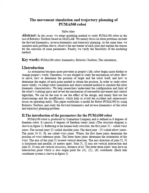
表1PUMA560机器人的连杆参数MATLAB 在机器人虚拟仿真实验教学中的应用收稿日期:2017-09-05资助项目:北京信息科技大学2017年度教学改革立项资助(2017JGYB01);北京信息科技大学2017年促进高校内涵发展-研究生教育质量工程类项目(5121723103)作者简介:刘相权(1972-),男(汉族),河北辛集人,北京信息科技大学机电工程学院,副教授,主要从事机械设计、机电控制方面的研究。
在机器人学课程的实验教学中,一方面由于机器人价格比较昂贵,不可能用许多实际的机器人来作为教学实验设备,另一方面,由于机器人的教学涉及大量数学运算,手工计算烦琐,采用虚拟仿真技术可以有效地提高教学的质量和效率,在实验教学中的作用越来越明显[1]。
本文以PUMA560机器人为研究对象,采用改进的D-H 法分析其结构和连杆参数,运用Robotics Toolbox 构建运动学模型并进行运动学仿真。
一、PUMA560机器人的结构及连杆参数PUMA560机器人是美国Unimation 公司生产的6自由度串联结构机器人,本文采用改进的D-H 法建立6个杆件的固接坐标系,如图1所示。
PUMA560机器人的杆件参数如表1所示,其中连杆扭角αi-1表示关节轴线i-1和关节轴线i 之间的夹角;连杆长度a i-1表示关节轴线i-1和关节轴线i 之间的公垂线长度;连杆转角θi 表示两公垂线a i-1和a i 之间的夹角;连杆距离d i 表示两公垂线a i-1和a i 之间的距离,对于旋转关节,θi 是关节变量[2]。
表1中a 2=0.4381,a 4=0.0203,d 2=0.1491,d 4=0.4331。
二、PUMA560机器人的运动学仿真1.机器人模型的建立。
在Robotics Toolbox 中,构建机器人模型关键在于构建各个杆件和关节,Link 函数用来创建一个杆件,其一般形式为:L=Link ([theta d a alpha sigma],CONVENTION )Link 函数的前4个参数依次为连杆转角θi ,连杆距离d i ,连杆长度a i-1,连杆扭角αi-1,第5个参数sigma 代表关节类型:0代表旋转关节,1代表平动关节,第6个参数CONVENTION 可以取'standard'或'modified',其中'standard'代表采用标准的D-H 方法,'modified'代表采用改进的D-H 方法[3]。
MATLAB在机器人虚拟仿真实验教学中的应用作者:刘相权来源:《教育教学论坛》2018年第15期摘要:本文简要介绍了MATLAB在机器人虚拟仿真实验教学中的基本应用。
以PUMA560机器人为研究对象,在MATLAB环境下,用Robotics Toolbox建立了该机器人的运动学模型,并对其进行求解,绘制了关节运动曲线和机器人末端运动轨迹。
通过使用虚拟仿真技术,使学生的创新能力和实践能力得到提高。
关键词:MATLAB;机器人;虚拟仿真;实验教学中图分类号:G642.0 文献标志码:A 文章编号:1674-9324(2018)15-0261-02在机器人学课程的实验教学中,一方面由于机器人价格比较昂贵,不可能用许多实际的机器人来作为教学实验设备,另一方面,由于机器人的教学涉及大量数学运算,手工计算烦琐,采用虚拟仿真技术可以有效地提高教学的质量和效率,在实验教学中的作用越来越明显[1]。
本文以PUMA560机器人为研究对象,采用改进的D-H法分析其结构和连杆参数,运用Robotics Toolbox构建运动学模型并进行运动学仿真。
一、PUMA560机器人的结构及连杆参数PUMA560机器人是美国Unimation公司生产的6自由度串联结构机器人,本文采用改进的D-H法建立6个杆件的固接坐标系,如图1所示。
二、PUMA560机器人的运动学仿真1.机器人模型的建立。
在Robotics Toolbox中,构建机器人模型关键在于构建各个杆件和关节,Link函数用来创建一个杆件,其一般形式为:L=Link([theta d a alpha sigma],CONVENTION)根据表1的数据,构建模型的仿真程序如下:三、结束语通过研究利用MATLAB软件进行虚拟仿真实验教学,克服了机器人实验设备数量不足的现状,把学生从烦琐的数值计算中解脱出来,实现了实验教学的创新,获得了良好的教学效果;同时激发了学生的学习兴趣,使其编程能力和创新能力均有所提高,充分发挥了学生在学习中的主体作用。
PUMA560机器人运动学分析——基于matlab程序的运动学求解求解PUMA560正向运动学解。
求解PUMA560逆向运动学解。
求解PUMA560的雅克比矩阵。
利用GUI创建运动分析界面。
姓名:xxx学号:201100800406学院:机电与信息工程学院专业:机械设计制造及其自动化年级2011指导教师:xx前言说明此次大作业,是我自己一点一点做的。
程序代码写好之后,感觉只是将代码写上去太过单调,而又不想将课本上或PPT上的基础知识部分复制上去,但我又想让自己的大作业有一点与众不同,所以我决定弄一个GUI界面。
开始对GUI一窍不通,经过几天的学习,终于有了点成果,但还是问题不断,有很多想法却难以去实现,考试在即,只能做成这样了,希望见谅。
目录前言说明 ................................................................................. - 1 -求解PUMA560正向运动学解 ............................................... - 2 -求解PUMA560逆向运动学解 ............................................... - 5 -求解PUMA560的雅克比矩阵 ............................................. - 15 -利用GUI创建运动分析界面................................................ - 22 -求解PUMA560正向运动学解在已知PUMA560各关节连杆DH参数,以及给定相应的关节变量之后,可以通过正向运动学求解出机械手末端抓手在基系内的位姿。
从而利用输入不同的关节变量组合,实现对PUMA560机器人的准确控制。
以下是利用matlab编写的求解PUMA560正向运动学解的函数zhenjie.m:function T=zhenjie(c1,c2,c3,c4,c5,c6)%求puma560正解a2=431.8;a3=20.32;d2=149.09;d4=433.07;c1=c1/180*pi;c2=c2/180*pi;c3=c3/180*pi;c4=c4/180*pi;c5=c5/180*pi;c6=c6/180*pi;A1=[cos(c1),-sin(c1),0,0;sin(c1),cos(c1),0,0;0,0,1,0;0,0,0,1];A2=[cos(c2),-sin(c2),0,0;0,0,1,d2;-sin(c2),-cos(c2),0,0;0,0,0,1];A3=[cos(c3),-sin(c3),0,a2;sin(c3),cos(c3),0,0;0,0,1,0;0,0,0,1];A4=[cos(c4),-sin(c4),0,a3;0,0,1,d4;-sin(c4),-cos(c4),0,0;0,0,0,1];A5= [cos(c5),-sin(c5),0,0;0,0,-1,0;sin(c5),cos(c5),0,0;0,0,0,1];A6=[cos(c6),-sin(c6),0,0;0,0,1,0;-sin(c6),-cos(c6),0,0;0,0,0,1];T=A1*A2*A3*A4*A5*A6end其中c1,c2,c3,c4,c5,c6,为分别输入的各关节变量,即连杆1、连杆2、连杆3、连杆4、连杆5、连杆6的关节转角,直接利用关节矩阵相乘得到机械手末端抓手在基系内的位姿。
通过MATLAB实现PUMA260机器人建模和运动分析摘要:针对PUMA260机器人,分析它的正运动学、逆运动学的问题。
采用标准D-H法对机器人建立6个关节的坐标系并获取D-H参数,并用MATLAB编程建立其运动的数学模型,同时实现正运动学、逆运动学求解和轨迹规划的仿真。
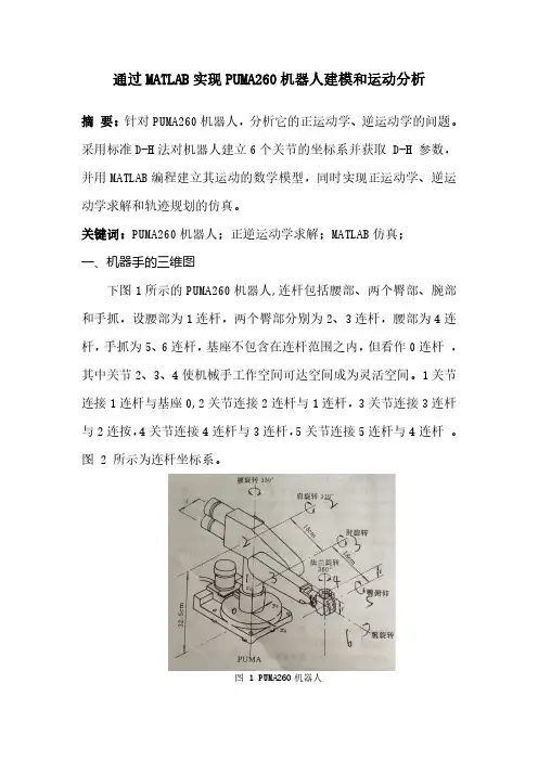
关键词:PUMA260机器人;正逆运动学求解;MATLAB仿真;一、机器手的三维图下图1所示的PUMA260机器人,连杆包括腰部、两个臀部、腕部和手抓,设腰部为1连杆,两个臀部分别为2、3连杆,腰部为4连杆,手抓为5、6连杆,基座不包含在连杆范围之内,但看作0连杆,其中关节2、3、4使机械手工作空间可达空间成为灵活空间。
1关节连接1连杆与基座0,2关节连接2连杆与1连杆,3关节连接3连杆与2连按,4关节连接4连杆与3连杆,5关节连接5连杆与4连杆。
图2所示为连杆坐标系。
图1PUMA260机器人二、建立连杆直角坐标系。
图2连杆直角坐标系三、根据坐标系确定D-H 表。
D-H 参数表四、利用MATLAB 编程求机械手仿真图。
clc;clear;%标准D-H 法建立机器人模型L1=Link([pi/20000],'standard');L2=Link([000-pi/20],'standard');L3=Link([0-101800],'standard');L4=Link([-pi/2018-pi/20],'standard');L5=Link([-pi/200-pi/20],'standard');L6=Link([000-pi/20],'standard');%将机器人命名为“ROBOT PUMA260”并用SerialLink 函数创建机器人bot=SerialLink([L1L2L3L4L5L6],'name','ROBOT PUMA260');bot.plot([000000]);连杆i θi di ai ɑi 运动范围190°32.500°-165~165°20°00-90°-105~105°30°L=-10180°-130~130°4-90°018-90°-180~180°5-90°00-90°-90~90°60°t=0-90°-165~165°图3PUMA260机器人运动仿真(起始位置时)%PUMA260机械手从Q1位置运动到Q2位置t=[0:0.01:1];%设定Q1位置参数和Q2位置参数Q1=[000000];Q2=[-pi/40pi/40-pi/40];%运用jtraj函数计算Q1、Q2点间的空间轨迹[q,qd,qdd]=jtraj(Q1,Q2,t);plot(bot,q);图4PUMA260机器人运动仿真(终止位置时)四、求PUMA260运动学正解和逆解。
基于MATLAB的PUMA机器人运动仿真研究
基于MATLAB的PUMA机器人运动仿真研究摘要:机器人运动学是机器人学的一个重要分支,是实现机器人运动控制的基础。
论文以D-H坐标系理论为基础对PUMA560机器人进行了参数设计,利用MATLAB机器人工具箱,对机器人的正运动学、逆运动学、轨迹规划进行了仿真。
Matlab仿真结果说明了所设计的参数的正确性,能够达到预定的目标。
关键词:机器人PUMA560 D-H坐标系运动学轨迹规划
机器人运动学的研究涉及大量的数学运算,计算工作相当繁锁。
因此,采用一些工具软件对其分析可大大提高工作效率,增加研究的灵活性和可操作性。
对机器人进行图形仿真,可以将机器人仿真的结果以图形的形式表示出来,从而直观地显示出机器人的运动情况,得到从数据曲线或数据本身难以分析出来的许多重要信息,还可以从图形上看到机器人在一定控制条件下的运动规律[1]。
论文首先设计了PUMA560机器人的各连杆参数,然后讨论了正、逆运动学算法,轨迹规划问题,最后在MATLAB环境下,运用Robotics Toolbox,编制简单的程序语句,快速完成了机器人得运动学仿真。
设机械手起始位置位于A点,qA=[000000],即表示机器人的各关节都处于零位置处。
机械手在B点和C点相对于基坐标系的位姿可用齐次变换矩阵TB和TC来表示。
图2所示为机械手臂在A点时的三维图形。
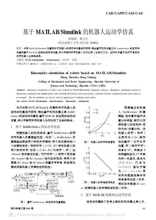
基于MAT LAB ΠSimulink 的机器人运动学仿真张晓超 董玉红(哈尔滨理工大学,哈尔滨150080)摘要 利用M AT LAB ΠS imulink 仿真软件对机器人的运动学仿真进行研究,提出基于机构仿真工具S imMechanics 的运动学仿真和基于M AT LAB 函数的运动学仿真,并以平面两关节机器人为例比较了各自的特点。
这两种仿真方法对于复杂多关节机器人也同样适用。
关键词:MAT LAB ΠSimulink SimMech anics 运动学 仿真中图分类号:TP 39119 文献标识码:A 文章编号:1671—3133(2005)增—0061—02K inematics simulation of robots based on MAT LAB ΠSimulinkZhang Xiaochao ,Dong Yuhong(College of Mechanical and Pow er E ngineering ,H aerbin U niversity ofScience and T echnology ,H aerbin 150080,CHN )Abstract K inematics simulations of robots were studied by M AT LAB ΠS imulink simulation s oftware.K inematics simulations based on mechanism simulation tool S imMechanics and on M AT LAB function were put forward ,and their features compared for tw o joints robot as an example.The tw o methods can als o be used in application to multiple joints robots.K ey w ords :MAT LAB ΠSimulink SimMech anics K inem atics Simulation 本文利用M AT LAB ΠSimulink 仿真软件对机器人的运动学仿真进行研究,提出基于机构仿真工具Sim Me 2chanics 的运动学仿真和基于M A T LAB 的函数的运动学仿真,并以平面两关节机器人为例比较了各自的特点。
一、安装Robotics Toolbox for MATLAB1、下载该工具箱:迅雷搜狗下载2、将压缩包解压到一个文件夹下面3、打开MATLAB,在File菜单下选择Set Path,打开如下对话框4、单击“Add With SubFolder”,选择上面的工具箱5、点击“Save”,然后点击“Close”。
这样就把工具箱的路径添加到MATLAB的路径中了,也就是工具箱安装了。
PUMA560的MATLAB仿真要建立PUMA560的机器人对象,首先我们要了解PUMA560的D-H参数,之后我们可以利用Robotics Toolbox工具箱中的link和robot函数来建立PUMA560的机器人对象。
其中link函数的调用格式:L = LINK([alpha A theta D])L =LINK([alpha A theta D sigma])L =LINK([alpha A theta D sigma offset])L =LINK([alpha A theta D], CONVENTION)L =LINK([alpha A theta D sigma], CONVENTION)L =LINK([alpha A theta D sigma offset], CONVENTION)参数CONVENTION可以取‘standard’和‘modified’,其中‘standard’代表采用标准的D-H参数,‘modified’代表采用改进的D-H参数。
参数‘alpha’代表扭转角,参数‘A’代表杆件长度,参数‘theta’代表关节角,参数‘D’代表横距,参数‘sigma’代表关节类型:0代表旋转关节,非0代表移动关节。
另外LINK还有一些数据域:LINK.alpha %返回扭转角LINK.A %返回杆件长度LINK.theta %返回关节角LINK.D %返回横距LINK.sigma %返回关节类型LINK.RP %返回‘R’(旋转)或‘P’(移动)LINK.mdh %若为标准D-H参数返回0,否则返回1LINK.offset %返回关节变量偏移LINK.qlim %返回关节变量的上下限[min max]LINK.islimit(q) %如果关节变量超限,返回-1, 0, +1LINK.I %返回一个3×3 对称惯性矩阵LINK.m %返回关节质量LINK.r %返回3×1的关节齿轮向量LINK.G %返回齿轮的传动比LINK.Jm %返回电机惯性LINK.B %返回粘性摩擦LINK.Tc %返回库仑摩擦LINK.dh return legacy DH rowLINK.dyn return legacy DYN row其中robot函数的调用格式:ROBOT %创建一个空的机器人对象ROBOT(robot) %创建robot的一个副本ROBOT(robot, LINK) %用LINK来创建新机器人对象来代替robotROBOT(LINK, ...) %用LINK来创建一个机器人对象ROBOT(DH, ...) %用D-H矩阵来创建一个机器人对象ROBOT(DYN, ...) %用DYN矩阵来创建一个机器人对象利用MATLAB中Robotics Toolbox工具箱中的transl、rotx、roty和rotz可以实现用齐次变换矩阵表示平移变换和旋转变换。
matlab实现PUMA机器人的工作空间PUMA机器人的工作空间主要有前3个关节决定,后3个关节决定姿态。
程序编写好了,请看运行结果!步长为20度步长为10度步长为5度步长为3度步长为2度步长为5度时的XY平面步长为5度时的XZ,YZ平面编写时的界面,为运行源代码如下:function varargout = mypuma(varargin)gui_Singleton = 1;gui_State = struct('gui_Name', mfilename, ... 'gui_Singleton', gui_Singleton, ...'gui_OpeningFcn', @mypuma_OpeningFcn, ...'gui_OutputFcn', @mypuma_OutputFcn, ...'gui_LayoutFcn', [], ...'gui_Callback', []);if nargin && ischar(varargin{1})gui_State.gui_Callback = str2func(varargin{1});endif nargout[varargout{1:nargout}] = gui_mainfcn(gui_State, varargin{:}); elsegui_mainfcn(gui_State, varargin{:});endhandles.output = hObject;guidata(hObject, handles);function varargout = mypuma_OutputFcn(hObject, eventdata, handles) varargout{1} = handles.output;%步长为20度时的工作空间,2个for循环就搞定function pushbutton1_Callback(hObject, eventdata, handles)hold off;for a=(-160:20:160)*pi/180for b=(-225:20:45)*pi/180x=431.8*cos(b)*cos(a)-149.09*sin(a);y=431.8*cos(b)*sin(a)+cos(a)*149.09;z=-431.8*sin(b);plot3(x,y,z,'b.');hold on;grid on;endendtitle('PUMA560 20deg 08S008103 ');%步长10度时的工作空间,2个for循环就搞定function pushbutton2_Callback(hObject, eventdata, handles) hold off;a2=431.8;d2=149.09;for a=(-160:10:160)*pi/180for b=(-225:10:45)*pi/180x=431.8*cos(b)*cos(a)-149.09*sin(a);y=431.8*cos(b)*sin(a)+cos(a)*149.09;z=-431.8*sin(b);plot3(x,y,z,'r.');hold on;grid on;endendtitle('PUMA560 10deg 08S008103 ');%步长为5度时的工作空间,2个for循环就搞定function pushbutton3_Callback(hObject, eventdata, handles) hold off;a2=431.8;d2=149.09;for a=(-160:5:160)*pi/180for b=(-225:5:45)*pi/180x=431.8*cos(b)*cos(a)-149.09*sin(a);y=431.8*cos(b)*sin(a)+cos(a)*149.09;z=-431.8*sin(b);plot3(x,y,z,'g.');hold on;grid on;endendtitle('PUMA560 5deg 08S008103 ');%步长为3度时的工作空间,2个for循环就搞定function pushbutton7_Callback(hObject, eventdata, handles) hold off;for a=(-160:3:160)*pi/180for b=(-225:3:45)*pi/180x=431.8*cos(b)*cos(a)-149.09*sin(a);y=431.8*cos(b)*sin(a)+cos(a)*149.09;z=-431.8*sin(b);plot3(x,y,z,'b.');hold on;grid on;endendtitle('PUMA560 3deg 08S008103 ');%步长为2度时的工作空间,2个for循环就搞定function pushbutton8_Callback(hObject, eventdata, handles) hold off;for a=(-160:2:160)*pi/180for b=(-225:2:45)*pi/180x=431.8*cos(b)*cos(a)-149.09*sin(a);y=431.8*cos(b)*sin(a)+cos(a)*149.09;z=-431.8*sin(b);plot3(x,y,z,'b.');hold on;grid on;endendtitle('PUMA560 2deg 08S008103 ');%步长为5度时的xy平面function pushbutton4_Callback(hObject, eventdata, handles) hold off;a2=431.8;d2=149.09;for a=(-160:5:160)*pi/180for b=(-225:5:45)*pi/180x=431.8*cos(b)*cos(a)-149.09*sin(a);y=431.8*cos(b)*sin(a)+cos(a)*149.09;z=-431.8*sin(b);plot(x,y,'g.');hold on;grid on;endendtitle('PUMA560 5degXY 08S008103 ');%步长为5度时的xz平面function pushbutton5_Callback(hObject, eventdata, handles) hold off;a2=431.8;d2=149.09;for a=(-160:5:160)*pi/180for b=(-225:5:45)*pi/180x=431.8*cos(b)*cos(a)-149.09*sin(a);y=431.8*cos(b)*sin(a)+cos(a)*149.09;z=-431.8*sin(b);plot(x,z,'g.');hold on;grid on;endendtitle('PUMA560 5degXZ 08S008103');%步长为5度时的yz平面function pushbutton6_Callback(hObject, eventdata, handles) hold off;a2=431.8;d2=149.09;for a=(-160:5:160)*pi/180for b=(-225:5:45)*pi/180x=431.8*cos(b)*cos(a)-149.09*sin(a);y=431.8*cos(b)*sin(a)+cos(a)*149.09;z=-431.8*sin(b);实用标准文案plot(y,z,'g.');hold on;grid on;endendtitle('PUMA560 5degY-Z 08S008103 '); 文档。
基于Matlab对于PUMA560机器人的运动空间分析研究沙漠;邓子龙【摘要】通过建立PUMA560机器人空间坐标系并确定连杆参数,利用D-H方法建立了运动学模型,在考虑每个连杆参数边界条件的基础上对其运动学方程求解,利用Robotics Toolbox模块对机器人运动进行了仿真,并利用MATLAB生成机器人工作空间图像,通过图像得到不同步长对于工作空间范围和密度的影响;通过对机器人工作空间及运动轨迹的分析,求得机器人杆长对其工作空间的影响系数,利用MATLAB对不同步长的工作空间范围及密度进行仿真、比较.结果可知:机器人的工作空间是由一近似的椭圆体构成,步长越小,密度与工作空间的精准度越高.为机器人的误差分析和结构优化设计提供理论依据,为机器人的动态控制以及机器人结构的动态特性研究奠定基础.【期刊名称】《机械制造与自动化》【年(卷),期】2016(045)002【总页数】5页(P156-159,183)【关键词】机器人;运动学;工作空间【作者】沙漠;邓子龙【作者单位】辽宁石油化工大学机械工程学院,辽宁抚顺113001;辽宁石油化工大学机械工程学院,辽宁抚顺113001【正文语种】中文【中图分类】TP241近年来,机器人技术在军事、航空航天、工农业生产及医疗等领域迅猛发展。
机器人按技术层次可以分为:固定程序控制机器人、示教再现机器人和智能机器人等。
目前机器人研究涉及到机构学、运动学、控制技术、传感技术等领域[1]。
由于机器人的研究涉及到庞大数学运算,计算工作繁琐复杂,常利用一些工具软件来提高对其分析的工作效率,并且可以增加运算的灵活性和准确性。
现利用MATLAB软件通用性好、计算绘图功能强大等特点,对PUMA560机器人的操作进行运动空间及轨迹的仿真分析得到相关图像数据,以便为实际操作和运算提供参考。
PUMA560机械人末端工作空间代表了机械手的活动范围,是表示机器人工作运动灵活性的一个非常重要指标。
基于MATLAB的PUMA-262型机械手控制系统设计与仿真任务书1.设计的主要任务及目标学生应通过本次毕业设计,综合运用所学过的基础理论知识,在深入了解反馈控制系统工作原理的基础上,掌握机械系统建模、分析及校正环节设计的基本过程;初步掌握运用MATLAB/Simulink相关模块进行控制系统设计与仿真的方法,为学生在毕业后从事机械控制系统设计工作打好基础。
2.设计的基本要求和内容(1)根据已有的PUMA-262型机械手相关资料,对其结构特点及工作原理进行分析;(2)建立系统的数学模型,分析系统的性能指标;(3)设计校正环节;(4)运用MATLAB/SIMULINK对系统进行仿真计算;(5)通过动态仿真设计优化系统参数;3.主要参考文献[1] 刘白燕等编,机电系统动态仿真-基于MATLAB/SIMULINK[M].北京:机械工业出版社,2005.7[2] 王积伟,吴振顺等著,控制工程基础[M].北京:高等教育出版社2001.8[3] 蔡自兴:机器人学清华大学出版社2000.94基于MATLAB的PUMA-262型机械手控制系统设计与仿真摘要;PUMA-262型机器人是美国UNIMATION公司制造的一种精密轻型关节式通用机器人。
本课题所研究的是基于MATLAB的PUMA-262型机械手系统控制进行设计与仿真,通过对该机械手的机构和传动原理进行了分析,建立了各关节的数学模型。
用MATLAB 做出系统的动态性能图,最后,设计数字控制对系统进行PID控制,根据系统性能指标的要求做出相应的离散响应图, 对控制系统进行校正和仿真,以验证最后结果。
关键字:数学模型,PUMA-262型机械手,控制器,PID校正,MATLAB仿真The PUMA-262 Robot Control Cystem Based On MATLABDesign And SimulationAbstract;PUMA-262 robot is a kind of UNIMATION companies in the United States manufacturing precision lightweight universal joint type robot. What this topic research is a PUMA - 262 robot system based on MATLAB control design and simulation, based on the mechanism and transmission principle of the manipulator are analyzed, Established the mathematical model of each joint. MATLAB to make the system dynamic performance figure, Finally, the design of digital control of PID control system, according to the requirement of the system performance index to make the corresponding discrete response figure, for calibration and control system is emulated, to verify the results.Keywords:mathematics mode;PUMA-262 robot; control box; PID correction ; matlab simulink目录1 绪论 (1)2 PUMA-262型机器人简介 (3)2.1 PUMA-262型机器人的传动原理 (5)2.2 PUMA-262型机器人的特点 (6)3 建立数学模型 (7)4控制系统的性能指标分析 (13)4.1控制系统的稳态误差 (14)4.2系统的抗干扰能力 (15)4.3控制系统稳定性 (16)4.4控制系统动态性能 (17)5 数字控制器与PID控制 (29)5.1关节1的控制系统模拟化设计 (29)5.2其他关节的控制系统模拟化设计 (34)6 用MATLAB进行仿真 (51)6.1在MATLAB环境下连续控制系统的时域图 (51)6.2 用MATLAB对系统进行仿真 (54)7总结与展望 (69)参考文献 (70)致谢 (71)附录 (72)1 绪论由于工业自动化的全面发展和科学技术的不断提高,对工作效率的提高迫在眉睫。
基于MATLAB的六自由度工业机器人运动分析及仿真六自由度工业机器人是一种常见的工业自动化设备,通过对其运动进行分析和仿真,可以对其性能进行评估和优化。
MATLAB是一种强大的数学计算软件,在工程领域广泛应用,可以帮助我们进行机器人的运动分析和仿真。
首先,我们可以使用MATLAB对六自由度机器人进行建模。
六自由度机器人具有六个自由度,分别为三个旋转自由度和三个平移自由度。
我们可以使用MATLAB的机器人工具箱来建立机器人的模型,并定义其关节参数和连接方式。
通过模型可以获得机器人的几何结构、动力学参数和运动学方程。
接下来,我们可以使用MATLAB进行机器人的运动分析。
运动分析是指通过对机器人的运动学和动力学进行计算,从而获得机器人的运动和力学特性。
机器人的运动学分析主要是利用机器人的几何结构来推导出末端执行器的位置和姿态。
可以使用MATLAB的运动学工具函数来计算机器人的正运动学和逆运动学。
机器人的动力学分析主要是研究机器人的运动和力学特性之间的关系。
动力学分析可以帮助我们确定机器人的运动特性和关节力矩。
我们可以使用MATLAB的动力学工具箱来建立机器人的动力学模型,并使用动力学工具函数来计算机器人的动力学性能。
最后,我们可以使用MATLAB进行机器人的仿真。
机器人的仿真是通过对机器人的动力学进行数值计算,来模拟机器人的运动和力学特性。
通过仿真可以验证机器人的设计和控制方案,并进行参数优化。
在MATLAB 中,我们可以使用数值计算函数和绘图函数来进行机器人的仿真和可视化。
总结起来,基于MATLAB的六自由度工业机器人运动分析及仿真可以帮助我们对机器人的运动和力学特性进行研究和优化。
通过建立机器人的模型,进行运动分析和动力学分析,以及进行仿真和可视化,可以帮助我们理解和改进机器人的性能,在工业自动化领域发挥更大的作用。
基于MATLAB/RoboticsToolbox的PUMA560机械臂仿真研究王娜【摘要】本文采用标准D-H法对六自由度关节机器人的机构和运动学进行分析,推导出正逆运动学变换公式。
在此基础上,本文运用Matlab机器人工具箱对机器人系统进行了运动仿真,研究了机器人在作业过程中的主要运动学指标的变化情况,十分直观地反映出机器人这一非线性耦合结构中各杆件和末端工作部分的运动状态,为机器人的具体研制、控制策略提供了理论依据。
【关键词】PUMA560机械臂;运动学;动力学;仿真1 PUMA560简介对机器人进行图形仿真,可以直观显示出机器人的运动情况,得到从数据曲线中难以分析出来的许多重要信息,并能从图形上看到机器人在一定控制条件下的运动规律。
从仿真软件中观察机器人工作程序的运行结果,就能分析出该机器人轨迹规划等的正确性和合理性,从而为离线编程提供有效的验证手段。
PUMA560 机械臂是一种示教机器人。
有六个自由度,包括6个旋转关節,模仿人的腰、肩、肘和手腕运动,能以规定的姿态到达工作范围内的任何一个点。
包括:臂体、控制器和示教器三个部分。
它的外观图如图1 所示。
2 PUMA560的空间坐标系建立PUMA560一般由移动关节和转动关节共同作用,组成机器人的操作臂,每个关节都有一个自由度。
在六自由度下,我们规定连杆0表示基座,关节1让基座0与连杆1相接,关节2让连杆1与连杆2相连接,以此类推。
如图2所示。
3 确定D-H坐标系PUMA560的6个关节全为转动关节如下:Xi轴:沿着Zi和Zi-1的公法线,指向离开Zi-1轴的方向;Yi轴:按右手直角坐标系法则制定;Zi轴:沿着i+1关节的运动轴;两连杆距di:Xi和Xi1两坐标轴的公法线距离;两杆夹角θi:Xi和Xi1两坐标轴的夹角;连杆长度ai:Zi和Zi-1两轴心线的公法线长度;连杆扭角αi:Zi和Zi-1两轴心线的夹角;所以相邻坐标系i和i-l的D-H变换矩阵为:6 结论本文利用 MATLAB Robotics Toolbox 建立了PUMA560机器人的三维模型,分析了它的正运动学、逆运动学和轨迹规划问题,验证了仿真的合理性。
基于MATLAB的PUMA机器人运动仿真研究
作者:邢广成张洛花
来源:《科技资讯》2011年第30期
摘要:机器人运动学是机器人学的一个重要分支,是实现机器人运动控制的基础。
论文以D-H坐标系理论为基础对PUMA560机器人进行了参数设计,利用MATLAB机器人工具箱,对机器人的正运动学、逆运动学、轨迹规划进行了仿真。
Matlab仿真结果说明了所设计的参数的正确性,能够达到预定的目标。
关键词:机器人 PUMA560 D-H坐标系运动学轨迹规划
中图分类号:TP24 文献标识码:A 文章编号:1672-3791(2011)10(c)-0000-00
机器人运动学的研究涉及大量的数学运算,计算工作相当繁锁。
因此,采用一些工具软件对其分析可大大提高工作效率,增加研究的灵活性和可操作性。
对机器人进行图形仿真,可以将机器人仿真的结果以图形的形式表示出来,从而直观地显示出机器人的运动情况,得到从数据曲线或数据本身难以分析出来的许多重要信息,还可以从图形上看到机器人在一定控制条件下的运动规律[1][5] 。
论文首先设计了PUMA560机器人的各连杆参数,然后讨论了正、逆运动学算法,轨迹规划问题,最后在 MATLAB 环境下,运用 Robotics Toolbox,编制简单的程序语句,快速完成了机器人得运动学仿真。
PUMA560机器人参数设计
1.1 D-H变换
为描述相邻杆件间平移和转动的关系,Denavit 和Hartenberg (1955)提出了一种为关节链中的每一杆件建立附体坐标系的矩阵方法[2]。
D-H 方法是为每个关节处的杆件坐标系建立 4*4
齐次变换矩阵(也称A矩阵),表示它与前一杆件坐标系的关系。
刚性杆件的 D-H 表示法取决于连杆的以下四个参数:-两连杆的夹角;-两连杆的距离;-连杆的长度 (即轴和轴间的最小距离) :-连杆的扭转角。
对于转动关节是关节变量,其余为关节参数(保持不变) :对于移动关节,是关节变量,其余为关节参数。
1。
2 PUMA560机器人的关节结构及其参数设计
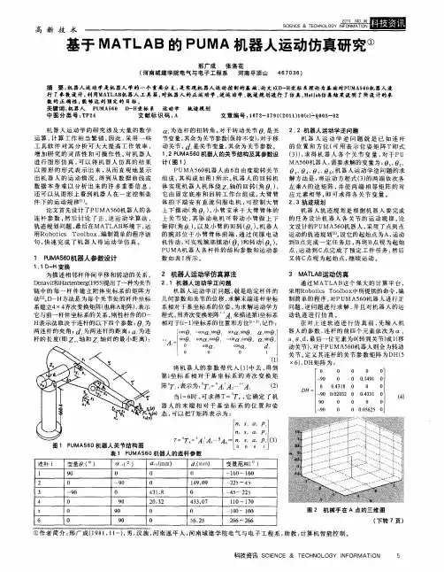
PUMA560机器人由6自由度旋转关节组成,其构成如图1所示。
机器人的回转机体实现机器人机体绕轴的回转(角),它由固定底座和回转工作台组成。
大臂臂体的下端安有直流伺服电机,可控制大臂上下摆动(角)。
小臂支承于大臂臂体的上关节处,其驱动电机可带动小臂做上下俯仰(角),以及小臂的回转()。
机器人的腕部位于小臂臂体前端,通过伺服电动机传动,可实现腕部摆动()和转动()。
PUMA机器人各杆件的结构参数和运动参数如表1所示[4]。
2.机器人运动学仿真算法
2。
1 机器人运动学正问题
机器人运动学正问题,就是给定杆件的几何参数和关节的位移,求解末端连杆坐标系相对于基坐标系的位姿。
为求解运动学方程式,用齐次变换矩阵来描述第i坐标系相对于(i-1)坐标系的位置和方位[2][3][4],记作:
(1)
将机器人的参数带代入(1)中去,得到第i坐标系相对于基坐标系的齐次变换矩阵,表示为:(2)
当i=6时,可求得T=,它确定了机器人的末端相对于基坐标系的位置和姿态,可以把T 矩阵表示为:= (3)
2.2 机器人运动学逆问题
机器人运动学逆问题就是已知连杆的位置和方位(可用表示位姿矩阵T即式(3)),求得机器人各个关节变量,对于PUMA560机器人,需要求解的变量为:。
机器人运动学逆问题的求解方法是:将运动方程式(3)的两端依次各左乘A的逆矩阵,并使两端相等矩阵的对应元素相等,即可求得各关节变量。
2.3 轨迹规划
机器人轨迹规划是根据机器人要完成的任务设计机器人各关节的运动规律。
论文设计的PUMA560机器人,采用了点到点运动的轨迹规划[2]。
设它的起始点为 A,运动到 B 点完成一定任务后,再将 B 点视为起始点,运动到 C点完成了预定工作任务,然后又将 C点视为起始点,继续运动。
3 MATLAB运动仿真
通过MATLAB这个强大的计算平台,采用Robotics Toolbox中所提供的命令,编制简单的程序,对PUMA560机器人进行正问题,逆问题进行求解,并且对机器人的运动轨迹进行仿真。
在对上述轨迹进行仿真前,先输入机器人的参数,连杆的前四个元素依次为、a、、d,最后一位元素为0(转到关节)或1(移动关节),对于PUMA560机器人则全为转动关节。
定义其连杆的关节参数矩阵为DH(5*6),DH矩阵为:
设机械手起始位置位于A点,qA=[0 0 0 0 0 0],即表示机器人的各关节都处于零位置处。
机械手在B点和C点相对于基坐标系的位姿可用齐次变换矩阵TB和TC来表示。
图2所示为机械手臂在A点时的三维图形。
可通过matlab编程来给出机器人由A运动到B,转动关节2和转动关节3的角度随时间变换的仿真图,如图3所示。
图4所示为末端关节沿x,y,z方向的运动轨迹。
取仿真时间为2s,采样间隔为0.056s。
从图3可以看出:在所取的仿真时间内,转动关节2由零逐渐变化到1.5708rad;转动关节3由零逐渐变化到-1.5708rad。
图4说明机器人由A运动到B,末端关节沿x,y,z方向位移矢量的变化轨迹,证明机器人可以实现不同方位的姿态。
通过仿真曲线可以观察到机器人从A运动到B时各关节的运动情况,且各关节运动情况均为正常,各连杆没有运动错位的情况,从而验证了所有连杆参数的合理性,且说明了各参数的设计能够实现预定的目标。
结语
论文基于D-H坐标系对PUMA560机器人进行了参数设计,分析了它的运动学问题和轨迹规划问题。
MATLAB仿真结果表明,只要机器人各关节角在给定范围内选择,得出的结果完全符合实际情况,说明参数设计合理,达到良好的效果。
参考文献
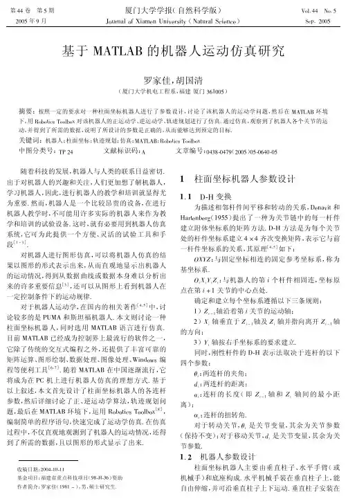
[1] 罗家佳,胡国清.基于Matlab的机器人运动学仿真[J].厦门大学学报(自然科学版),Vol.44 No.5.
[2] 蔡自兴.机器人学[M].北京:清华大学出版社,2000.
[3] 干民耀,马骏骑等.基于Matlab的Puma机器人运动学仿真[J].昆明理工大学学报(理工版),Vol.28 No.6.。