Maturation of spatial-frequency and orientation selectivity of primary visual cortex

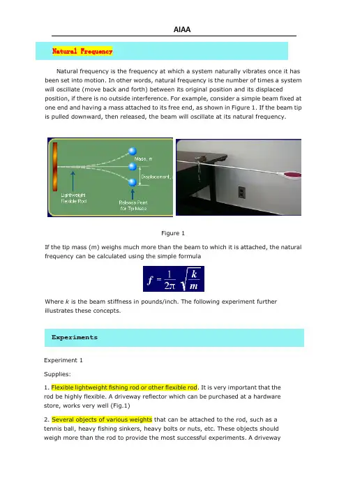
Natural frequency is the frequency at which a system naturally vibrates once it has been set into motion. In other words, natural frequency is the number of times a system will oscillate (move back and forth) between its original position and its displaced position, if there is no outside interference. For example, consider a simple beam fixed at one end and having a mass attached to its free end, as shown in Figure 1. If the beam tip is pulled downward, then released, the beam will oscillate at its natural frequency.Figure 1If the tip mass (m) weighs much more than the beam to which it is attached, the natural frequency can be calculated using the simple formulaWhere k is the beam stiffness in pounds/inch. The following experiment further illustrates these concepts.ExperimentsExperiment 1Supplies:1. Flexible lightweight fishing rod or other flexible rod. It is very important thatthe rod be highly flexible. A driveway reflector which can be purchased at a hardware store, works very well (Fig.1)2. Several objects of various weights that can be attached to the rod, such as a tennis ball, heavy fishing sinkers, heavy bolts or nuts, etc. These objects should weigh more than the rod to provide the most successful experiments. A drivewayreflector as shown in Figures 1 and 2 provides a convenient location for attaching weights3. Table to which the rod can be attached.4. C-clamp for fastening the rod to the edge of the table.5. Stopwatch or clock with capability to indicate seconds.Procedure:1. Clamp one end of the flexible rod to the table. Start without any tip weights. If a driveway reflector rod is used, the reflector should be removed initially.2. Pull the end of the rod downward, and then release it. If the rod moves slowly enough, count the number of oscillations (rod moving through complete cycle and back to release point) that occur in 30 seconds. The frequency is the number of oscillations divided by seconds.3. Now attach one of the weights to the free end of the rod, (such as the reflector tip mass in figure 1) and again pull it downward then release it. Count the number of oscillations and divide by the time to get frequency.4. Repeat step 3 for different tip weights. Plot frequency vs. tip weight. How does frequency change with the weight?5. Calculate the natural frequency and compare to the experiment described in steps 3 and 4 using the following procedure:(a). Place a yardstick near the free end of the flexible rod, with one end of the yardstick resting on the floor. Note the location of the end of the rod and mark it on the yardstick.(b). Attach several different weights to the end of the rod and measure the distance (x) that the end of the rod moves downward (see Figure 2) for each weight. Graph weight versus displacement. The stiffness K is the slope of this graph (rise/run), units (lb/in).Figure 2(c). Calculate the natural frequency using the formulawhere stiffness k is measured in step (b) and m equals the tip weight divided by 386.1. How does this frequency compare to the measured natural frequency?(d). Repeat steps (c) for different tip weights. Plot frequency vs. tip weight. How does this graph compare to the experiment results from step 4? More advanced students should overlay the two graphs.ResonanceResonance is the buildup of large vibration amplitude that occurs when a structure or an object is excited at its natural frequency. Resonance can be either desirable or undesirable. Acoustic resonance, a desirable resonance, occurs in many different musical instruments. It also occurs in auditoriums. Undesirable mechanical resonance can cause bridges to collapse, aircraft wings to break, and machinery to break or malfunction. For example, the Tacoma Narrows Bridge experienced large vibration amplitudes and catastrophic structural failure due to wind gusts.Experiment 2: Resonance and Resonating Chambers (Tuning Fork withSoda Can)Supplies:1.Clean, empty soda can2 Tuning forkDirections:Tap the fork and listen. Hold it over the opening of the can as shown in Figure 3 and listen.Notice that the sound gets louder when it is held over the opening.Figure 3Explanation:The can is a hollow container with an opening and is called a resonator. Its shape acts like a resonating chamber, like a drum or the bell of a tuba. The vibrating tuning fork held near the opening causes the can and the air in the can to vibrate. This is called resonance. The sound becomes intensified and amplified.References:Holiday and Resnick “Physics”。

1.BackgroundHoward Earl Gardener’s work has been marked by a desire not to just describe the world but to help to create the condition to change it. The scale of his contribution can be gauged from following comments in his introduction to the tenth anniversary edition of Howard Gardener’s classic work Frames Of Mind. The theory of multiple intelligences :霍华德厄尔加德纳的研究不只是描述这个世界,而是造条件去改变它。

他的贡献在十周年纪念版的《霍华德加德纳的经典智力结构》这本书中有所介绍。

多元智能的理论:In the heyday of the psychometric and behaviorist eras, it was generally believed that intelligence was a single entity that was inherited; and that human beings – initially a blank slate – could be trained to learn anything, provided that it was presented in an appropriate way. Nowadays an intelligences, quite independent of each other; that each intelligence has its own strengths and constraints; that the mind is far from unencumbered at birth; and that it is unexpectedly difficult to teach things that go against early’naïve’ theories of that challenge the natural lines of force within an intelligence and its matching domains.全盛时期的心理和行为主义时代,人们普遍认为,智力是一个单一的实体,是可以继承的;而人类——最初就像一张白纸可以通过训练学习任何东西,只需要有一个适当的方式。

IEEE Std 1159-1995 IEEE Recommended Practice for Monitoring Electric Power QualitySponsorIEEE Standards Coordinating Committee 22 onPower QualityApproved June 14, 1995IEEE Standards BoardAbstract: The monitoring of electric power quality of ac power systems, definitions of power quality terminology, impact of poor power quality on utility and customer equipment, and the measurement of electromagnetic phenomena are covered.Keywords: data interpretation, electric power quality, electromagnetic phenomena, monitoring, power quality definitionsIEEE Standards documents are developed within the Technical Committees of the IEEE Societies and the Standards Coordinating Committees of the IEEE Standards Board. Members of the committees serve voluntarily and without compensation. They are not necessarily members of the Institute. The standards developed within IEEE represent a consensus of the broad expertise on the subject within the Institute as well as those activities outside of IEEE that have expressed an interest in partici-pating in the development of the standard.Use of an IEEE Standard is wholly voluntary. The existence of an IEEE Standard does not imply that there are no other ways to produce, test, measure, purchase, mar-ket, or provide other goods and services related to the scope of the IEEE Standard. Furthermore, the viewpoint expressed at the time a standard is approved and issued is subject to change brought about through developments in the state of the art and com-ments received from users of the standard. Every IEEE Standard is subjected to review at least every Þve years for revision or reafÞrmation. When a document is more than Þve years old and has not been reafÞrmed, it is reasonable to conclude that its contents, although still of some value, do not wholly reßect the present state of the art. Users are cautioned to check to determine that they have the latest edition of any IEEE Standard.Comments for revision of IEEE Standards are welcome from any interested party, regardless of membership afÞliation with IEEE. Suggestions for changes in docu-ments should be in the form of a proposed change of text, together with appropriate supporting comments.Interpretations: Occasionally questions may arise regarding the meaning of portions of standards as they relate to speciÞc applications. When the need for interpretations is brought to the attention of IEEE, the Institute will initiate action to prepare appro-priate responses. Since IEEE Standards represent a consensus of all concerned inter-ests, it is important to ensure that any interpretation has also received the concurrence of a balance of interests. For this reason IEEE and the members of its technical com-mittees are not able to provide an instant response to interpretation requests except in those cases where the matter has previously received formal consideration.Comments on standards and requests for interpretations should be addressed to:Secretary, IEEE Standards Board445 Hoes LaneP.O. Box 1331Piscataway, NJ 08855-1331USAIntroduction(This introduction is not part of IEEE Std 1159-1995, IEEE Recommended Practice for Monitoring Electric Power Quality.)This recommended practice was developed out of an increasing awareness of the difÞculty in comparing results obtained by researchers using different instruments when seeking to characterize the quality of low-voltage power systems. One of the initial goals was to promote more uniformity in the basic algorithms and data reduction methods applied by different instrument manufacturers. This proved difÞcult and was not achieved, given the free market principles under which manufacturers design and market their products. However, consensus was achieved on the contents of this recommended practice, which provides guidance to users of monitoring instruments so that some degree of comparisons might be possible.An important Þrst step was to compile a list of power quality related deÞnitions to ensure that contributing parties would at least speak the same language, and to provide instrument manufacturers with a common base for identifying power quality phenomena. From that starting point, a review of the objectives of moni-toring provides the necessary perspective, leading to a better understanding of the means of monitoringÑthe instruments. The operating principles and the application techniques of the monitoring instruments are described, together with the concerns about interpretation of the monitoring results. Supporting information is provided in a bibliography, and informative annexes address calibration issues.The Working Group on Monitoring Electric Power Quality, which undertook the development of this recom-mended practice, had the following membership:J. Charles Smith, Chair Gil Hensley, SecretaryLarry Ray, Technical EditorMark Andresen Thomas Key John RobertsVladi Basch Jack King Anthony St. JohnRoger Bergeron David Kreiss Marek SamotyjJohn Burnett Fran•ois Martzloff Ron SmithJohn Dalton Alex McEachern Bill StuntzAndrew Dettloff Bill Moncrief John SullivanDave GrifÞth Allen Morinec David VannoyThomas Gruzs Ram Mukherji Marek WaclawlakErich Gunther Richard Nailen Daniel WardMark Kempker David Pileggi Steve WhisenantHarry RauworthIn addition to the working group members, the following people contributed their knowledge and experience to this document:Ed Cantwell Christy Herig Tejindar SinghJohn Curlett Allan Ludbrook Maurice TetreaultHarshad MehtaiiiThe following persons were on the balloting committee:James J. Burke David Kreiss Jacob A. RoizDavid A. Dini Michael Z. Lowenstein Marek SamotyjW. Mack Grady Fran•ois D. Martzloff Ralph M. ShowersDavid P. Hartmann Stephen McCluer J. C. SmithMichael Higgins A. McEachern Robert L. SmithThomas S. Key W. A. Moncrief Daniel J. WardJoseph L. KoepÞnger P. Richman Charles H. WilliamsJohn M. RobertsWhen the IEEE Standards Board approved this standard on June 14, 1995, it had the following membership:E. G. ÒAlÓ Kiener, Chair Donald C. Loughry,Vice ChairAndrew G. Salem,SecretaryGilles A. Baril Richard J. Holleman Marco W. MigliaroClyde R. Camp Jim Isaak Mary Lou PadgettJoseph A. Cannatelli Ben C. Johnson John W. PopeStephen L. Diamond Sonny Kasturi Arthur K. ReillyHarold E. Epstein Lorraine C. Kevra Gary S. RobinsonDonald C. Fleckenstein Ivor N. Knight Ingo RuschJay Forster*Joseph L. KoepÞnger*Chee Kiow TanDonald N. Heirman D. N. ÒJimÓ Logothetis Leonard L. TrippL. Bruce McClung*Member EmeritusAlso included are the following nonvoting IEEE Standards Board liaisons:Satish K. AggarwalRichard B. EngelmanRobert E. HebnerChester C. TaylorRochelle L. SternIEEE Standards Project EditorivContentsCLAUSE PAGE 1.Overview (1)1.1Scope (1)1.2Purpose (2)2.References (2)3.Definitions (2)3.1Terms used in this recommended practice (2)3.2Avoided terms (7)3.3Abbreviations and acronyms (8)4.Power quality phenomena (9)4.1Introduction (9)4.2Electromagnetic compatibility (9)4.3General classification of phenomena (9)4.4Detailed descriptions of phenomena (11)5.Monitoring objectives (24)5.1Introduction (24)5.2Need for monitoring power quality (25)5.3Equipment tolerances and effects of disturbances on equipment (25)5.4Equipment types (25)5.5Effect on equipment by phenomena type (26)6.Measurement instruments (29)6.1Introduction (29)6.2AC voltage measurements (29)6.3AC current measurements (30)6.4Voltage and current considerations (30)6.5Monitoring instruments (31)6.6Instrument power (34)7.Application techniques (35)7.1Safety (35)7.2Monitoring location (38)7.3Equipment connection (41)7.4Monitoring thresholds (43)7.5Monitoring period (46)8.Interpreting power monitoring results (47)8.1Introduction (47)8.2Interpreting data summaries (48)8.3Critical data extraction (49)8.4Interpreting critical events (51)8.5Verifying data interpretation (59)vANNEXES PAGE Annex A Calibration and self testing (informative) (60)A.1Introduction (60)A.2Calibration issues (61)Annex B Bibliography (informative) (63)B.1Definitions and general (63)B.2Susceptibility and symptomsÑvoltage disturbances and harmonics (65)B.3Solutions (65)B.4Existing power quality standards (67)viIEEE Recommended Practice for Monitoring Electric Power Quality1. Overview1.1 ScopeThis recommended practice encompasses the monitoring of electric power quality of single-phase and polyphase ac power systems. As such, it includes consistent descriptions of electromagnetic phenomena occurring on power systems. The document also presents deÞnitions of nominal conditions and of deviations from these nominal conditions, which may originate within the source of supply or load equipment, or from interactions between the source and the load.Brief, generic descriptions of load susceptibility to deviations from nominal conditions are presented to identify which deviations may be of interest. Also, this document presents recommendations for measure-ment techniques, application techniques, and interpretation of monitoring results so that comparable results from monitoring surveys performed with different instruments can be correlated.While there is no implied limitation on the voltage rating of the power system being monitored, signal inputs to the instruments are limited to 1000 Vac rms or less. The frequency ratings of the ac power systems being monitored are in the range of 45Ð450 Hz.Although it is recognized that the instruments may also be used for monitoring dc supply systems or data transmission systems, details of application to these special cases are under consideration and are not included in the scope. It is also recognized that the instruments may perform monitoring functions for envi-ronmental conditions (temperature, humidity, high frequency electromagnetic radiation); however, the scope of this document is limited to conducted electrical parameters derived from voltage or current measure-ments, or both.Finally, the deÞnitions are solely intended to characterize common electromagnetic phenomena to facilitate communication between various sectors of the power quality community. The deÞnitions of electromagnetic phenomena summarized in table 2 are not intended to represent performance standards or equipment toler-ances. Suppliers of electricity may utilize different thresholds for voltage supply, for example, than the ±10% that deÞnes conditions of overvoltage or undervoltage in table 2. Further, sensitive equipment may mal-function due to electromagnetic phenomena not outside the thresholds of the table 2 criteria.1IEEEStd 1159-1995IEEE RECOMMENDED PRACTICE FOR 1.2 PurposeThe purpose of this recommended practice is to direct users in the proper monitoring and data interpretation of electromagnetic phenomena that cause power quality problems. It deÞnes power quality phenomena in order to facilitate communication within the power quality community. This document also forms the con-sensus opinion about safe and acceptable methods for monitoring electric power systems and interpreting the results. It further offers a tutorial on power system disturbances and their common causes.2. ReferencesThis recommended practice shall be used in conjunction with the following publications. When the follow-ing standards are superseded by an approved revision, the revision shall apply.IEC 1000-2-1 (1990), Electromagnetic Compatibility (EMC)ÑPart 2 Environment. Section 1: Description of the environmentÑelectromagnetic environment for low-frequency conducted disturbances and signaling in public power supply systems.1IEC 50(161)(1990), International Electrotechnical V ocabularyÑChapter 161: Electromagnetic Compatibility. IEEE Std 100-1992, IEEE Standard Dictionary of Electrical and Electronic Terms (ANSI).2IEEE Std 1100-1992, IEEE Recommended Practice for Powering and Grounding Sensitive Electronic Equipment (Emerald Book) (ANSI).3. DeÞnitionsThe purpose of this clause is to present concise deÞnitions of words that convey the basic concepts of power quality monitoring. These terms are listed below and are expanded in clause 4. The power quality commu-nity is also pervaded by terms that have no scientiÞc deÞnition. A partial listing of these words is included in 3.2; use of these terms in the power quality community is discouraged. Abbreviations and acronyms that are employed throughout this recommended practice are listed in 3.3.3.1 Terms used in this recommended practiceThe primary sources for terms used are IEEE Std 100-19923 indicated by (a), and IEC 50 (161)(1990) indi-cated by (b). Secondary sources are IEEE Std 1100-1992 indicated by (c), IEC-1000-2-1 (1990) indicated by (d) and UIE -DWG-3-92-G [B16]4. Some referenced deÞnitions have been adapted and modiÞed in order to apply to the context of this recommended practice.3.1.1 accuracy: The freedom from error of a measurement. Generally expressed (perhaps erroneously) as percent inaccuracy. Instrument accuracy is expressed in terms of its uncertaintyÑthe degree of deviation from a known value. An instrument with an uncertainty of 0.1% is 99.9% accurate. At higher accuracy lev-els, uncertainty is typically expressed in parts per million (ppm) rather than as a percentage.1IEC publications are available from IEC Sales Department, Case Postale 131, 3, rue de VarembŽ, CH-1211, Gen•ve 20, Switzerland/ Suisse. IEC publications are also available in the United States from the Sales Department, American National Standards Institute, 11 West 42nd Street, 13th Floor, New York, NY 10036, USA.2IEEE publications are available from the Institute of Electrical and Electronics Engineers, 445 Hoes Lane, P.O. Box 1331, Piscataway, NJ 08855-1331, USA.3Information on references can be found in clause 2.4The numbers in brackets correspond to those bibliographical items listed in annex B.2IEEE MONITORING ELECTRIC POWER QUALITY Std 1159-1995 3.1.2 accuracy ratio: The ratio of an instrumentÕs tolerable error to the uncertainty of the standard used to calibrate it.3.1.3 calibration: Any process used to verify the integrity of a measurement. The process involves compar-ing a measuring instrument to a well defined standard of greater accuracy (a calibrator) to detect any varia-tions from specified performance parameters, and making any needed compensations. The results are then recorded and filed to establish the integrity of the calibrated instrument.3.1.4 common mode voltage: A voltage that appears between current-carrying conductors and ground.b The noise voltage that appears equally and in phase from each current-carrying conductor to ground.c3.1.5 commercial power: Electrical power furnished by the electric power utility company.c3.1.6 coupling: Circuit element or elements, or network, that may be considered common to the input mesh and the output mesh and through which energy may be transferred from one to the other.a3.1.7 current transformer (CT): An instrument transformer intended to have its primary winding con-nected in series with the conductor carrying the current to be measured or controlled.a3.1.8 dip: See: sag.3.1.9 dropout: A loss of equipment operation (discrete data signals) due to noise, sag, or interruption.c3.1.10 dropout voltage: The voltage at which a device fails to operate.c3.1.11 electromagnetic compatibility: The ability of a device, equipment, or system to function satisfacto-rily in its electromagnetic environment without introducing intolerable electromagnetic disturbances to any-thing in that environment.b3.1.12 electromagnetic disturbance: Any electromagnetic phenomena that may degrade the performance of a device, equipment, or system, or adversely affect living or inert matter.b3.1.13 electromagnetic environment: The totality of electromagnetic phenomena existing at a given location.b3.1.14 electromagnetic susceptibility: The inability of a device, equipment, or system to perform without degradation in the presence of an electromagnetic disturbance.NOTEÑSusceptibility is a lack of immunity.b3.1.15 equipment grounding conductor: The conductor used to connect the noncurrent-carrying parts of conduits, raceways, and equipment enclosures to the grounded conductor (neutral) and the grounding elec-trode at the service equipment (main panel) or secondary of a separately derived system (e.g., isolation transformer). See Section 100 in ANSI/NFPA 70-1993 [B2].3.1.16 failure mode: The effect by which failure is observed.a3.1.17 ßicker: Impression of unsteadiness of visual sensation induced by a light stimulus whose luminance or spectral distribution fluctuates with time.b3.1.18 frequency deviation: An increase or decrease in the power frequency. The duration of a frequency deviation can be from several cycles to several hours.c Syn.: power frequency variation.3.1.19 fundamental (component): The component of an order 1 (50 or 60 Hz) of the Fourier series of a periodic quantity.b3IEEEStd 1159-1995IEEE RECOMMENDED PRACTICE FOR 3.1.20 ground: A conducting connection, whether intentional or accidental, by which an electric circuit or piece of equipment is connected to the earth, or to some conducting body of relatively large extent that serves in place of the earth.NOTEÑ It is used for establishing and maintaining the potential of the earth (or of the conducting body) or approxi-mately that potential, on conductors connected to it, and for conducting ground currents to and from earth (or the con-ducting body).a3.1.21 ground loop: In a radial grounding system, an undesired conducting path between two conductive bodies that are already connected to a common (single-point) ground.3.1.22 harmonic (component): A component of order greater than one of the Fourier series of a periodic quantity.b3.1.23 harmonic content: The quantity obtained by subtracting the fundamental component from an alter-nating quantity.a3.1.24 immunity (to a disturbance): The ability of a device, equipment, or system to perform without deg-radation in the presence of an electromagnetic disturbance.b3.1.25 impulse: A pulse that, for a given application, approximates a unit pulse.b When used in relation to the monitoring of power quality, it is preferred to use the term impulsive transient in place of impulse.3.1.26 impulsive transient: A sudden nonpower frequency change in the steady-state condition of voltage or current that is unidirectional in polarity (primarily either positive or negative).3.1.27 instantaneous: A time range from 0.5Ð30 cycles of the power frequency when used to quantify the duration of a short duration variation as a modifier.3.1.28 interharmonic (component): A frequency component of a periodic quantity that is not an integer multiple of the frequency at which the supply system is designed to operate operating (e.g., 50 Hz or 60 Hz).3.1.29 interruption, momentary (power quality monitoring): A type of short duration variation. The complete loss of voltage (< 0.1 pu) on one or more phase conductors for a time period between 0.5 cycles and 3 s.3.1.30 interruption, sustained (electric power systems): Any interruption not classified as a momentary interruption.3.1.31 interruption, temporary (power quality monitoring):A type of short duration variation. The com-plete loss of voltage (< 0.1 pu) on one or more phase conductors for a time period between 3 s and 1 min.3.1.32 isolated ground: An insulated equipment grounding conductor run in the same conduit or raceway as the supply conductors. This conductor may be insulated from the metallic raceway and all ground points throughout its length. It originates at an isolated ground-type receptacle or equipment input terminal block and terminates at the point where neutral and ground are bonded at the power source. See Section 250-74, Exception #4 and Exception in Section 250-75 in ANSI/NFPA 70-1993 [B2].3.1.33 isolation: Separation of one section of a system from undesired influences of other sections.c3.1.34 long duration voltage variation:See: voltage variation, long duration.3.1.35 momentary (power quality monitoring): A time range at the power frequency from 30 cycles to 3 s when used to quantify the duration of a short duration variation as a modifier.4IEEE MONITORING ELECTRIC POWER QUALITY Std 1159-1995 3.1.36 momentary interruption:See: interruption, momentary.3.1.37 noise: Unwanted electrical signals which produce undesirable effects in the circuits of the control systems in which they occur.a (For this document, control systems is intended to include sensitive electronic equipment in total or in part.)3.1.38 nominal voltage (Vn): A nominal value assigned to a circuit or system for the purpose of conve-niently designating its voltage class (as 120/208208/120, 480/277, 600).d3.1.39 nonlinear load: Steady-state electrical load that draws current discontinuously or whose impedance varies throughout the cycle of the input ac voltage waveform.c3.1.40 normal mode voltage: A voltage that appears between or among active circuit conductors, but not between the grounding conductor and the active circuit conductors.3.1.41 notch: A switching (or other) disturbance of the normal power voltage waveform, lasting less than 0.5 cycles, which is initially of opposite polarity than the waveform and is thus subtracted from the normal waveform in terms of the peak value of the disturbance voltage. This includes complete loss of voltage for up to 0.5 cycles [B13].3.1.42 oscillatory transient: A sudden, nonpower frequency change in the steady-state condition of voltage or current that includes both positive or negative polarity value.3.1.43 overvoltage: When used to describe a specific type of long duration variation, refers to a measured voltage having a value greater than the nominal voltage for a period of time greater than 1 min. Typical val-ues are 1.1Ð1.2 pu.3.1.44 phase shift: The displacement in time of one waveform relative to another of the same frequency and harmonic content.c3.1.45 potential transformer (PT): An instrument transformer intended to have its primary winding con-nected in shunt with a power-supply circuit, the voltage of which is to be measured or controlled. Syn.: volt-age transformer.a3.1.46 power disturbance: Any deviation from the nominal value (or from some selected thresholds based on load tolerance) of the input ac power characteristics.c3.1.47 power quality: The concept of powering and grounding sensitive equipment in a manner that is suit-able to the operation of that equipment.cNOTEÑWithin the industry, alternate definitions or interpretations of power quality have been used, reflecting different points of view. Therefore, this definition might not be exclusive, pending development of a broader consensus.3.1.48 precision: Freedom from random error.3.1.49 pulse: An abrupt variation of short duration of a physical an electrical quantity followed by a rapid return to the initial value.3.1.50 random error: Error that is not repeatable, i.e., noise or sensitivity to changing environmental factors. NOTEÑFor most measurements, the random error is small compared to the instrument tolerance.3.1.51 sag: A decrease to between 0.1 and 0.9 pu in rms voltage or current at the power frequency for dura-tions of 0.5 cycle to 1 min. Typical values are 0.1 to 0.9 pu.b See: dip.IEEEStd 1159-1995IEEE RECOMMENDED PRACTICE FOR NOTEÑTo give a numerical value to a sag, the recommended usage is Òa sag to 20%,Ó which means that the line volt-age is reduced down to 20% of the normal value, not reduced by 20%. Using the preposition ÒofÓ (as in Òa sag of 20%,Óor implied by Òa 20% sagÓ) is deprecated.3.1.52 shield: A conductive sheath (usually metallic) normally applied to instrumentation cables, over the insulation of a conductor or conductors, for the purpose of providing means to reduce coupling between the conductors so shielded and other conductors that may be susceptible to, or that may be generating unwanted electrostatic or electromagnetic fields (noise).c3.1.53 shielding: The use of a conducting and/or ferromagnetic barrier between a potentially disturbing noise source and sensitive circuitry. Shields are used to protect cables (data and power) and electronic cir-cuits. They may be in the form of metal barriers, enclosures, or wrappings around source circuits and receiv-ing circuits.c3.1.54 short duration voltage variation:See: voltage variation, short duration.3.1.55 slew rate: Rate of change of ac voltage, expressed in volts per second a quantity such as volts, fre-quency, or temperature.a3.1.56 sustained: When used to quantify the duration of a voltage interruption, refers to the time frame asso-ciated with a long duration variation (i.e., greater than 1 min).3.1.57 swell: An increase in rms voltage or current at the power frequency for durations from 0.5 cycles to 1 min. Typical values are 1.1Ð1.8 pu.3.1.58 systematic error: The portion of error that is repeatable, i.e., zero error, gain or scale error, and lin-earity error.3.1.59 temporary interruption:See: interruption, temporary.3.1.60 tolerance: The allowable variation from a nominal value.3.1.61 total harmonic distortion disturbance level: The level of a given electromagnetic disturbance caused by the superposition of the emission of all pieces of equipment in a given system.b The ratio of the rms of the harmonic content to the rms value of the fundamental quantity, expressed as a percent of the fun-damental [B13].a Syn.: distortion factor.3.1.62 traceability: Ability to compare a calibration device to a standard of even higher accuracy. That stan-dard is compared to another, until eventually a comparison is made to a national standards laboratory. This process is referred to as a chain of traceability.3.1.63 transient: Pertaining to or designating a phenomenon or a quantity that varies between two consecu-tive steady states during a time interval that is short compared to the time scale of interest. A transient can be a unidirectional impulse of either polarity or a damped oscillatory wave with the first peak occurring in either polarity.b3.1.64 undervoltage: A measured voltage having a value less than the nominal voltage for a period of time greater than 1 min when used to describe a specific type of long duration variation, refers to. Typical values are 0.8Ð0.9 pu.3.1.65 voltage change: A variation of the rms or peak value of a voltage between two consecutive levels sustained for definite but unspecified durations.d3.1.66 voltage dip:See: sag.IEEE MONITORING ELECTRIC POWER QUALITY Std 1159-1995 3.1.67 voltage distortion: Any deviation from the nominal sine wave form of the ac line voltage.3.1.68 voltage ßuctuation: A series of voltage changes or a cyclical variation of the voltage envelope.d3.1.69 voltage imbalance (unbalance), polyphase systems: The maximum deviation among the three phases from the average three-phase voltage divided by the average three-phase voltage. The ratio of the neg-ative or zero sequence component to the positive sequence component, usually expressed as a percentage.a3.1.70 voltage interruption: Disappearance of the supply voltage on one or more phases. Usually qualified by an additional term indicating the duration of the interruption (e.g., momentary, temporary, or sustained).3.1.71 voltage regulation: The degree of control or stability of the rms voltage at the load. Often specified in relation to other parameters, such as input-voltage changes, load changes, or temperature changes.c3.1.72 voltage variation, long duration: A variation of the rms value of the voltage from nominal voltage for a time greater than 1 min. Usually further described using a modifier indicating the magnitude of a volt-age variation (e.g., undervoltage, overvoltage, or voltage interruption).3.1.73 voltage variation, short duration: A variation of the rms value of the voltage from nominal voltage for a time greater than 0.5 cycles of the power frequency but less than or equal to 1 minute. Usually further described using a modifier indicating the magnitude of a voltage variation (e.g. sag, swell, or interruption) and possibly a modifier indicating the duration of the variation (e.g., instantaneous, momentary, or temporary).3.1.74 waveform distortion: A steady-state deviation from an ideal sine wave of power frequency princi-pally characterized by the spectral content of the deviation [B13].3.2 Avoided termsThe following terms have a varied history of usage, and some may have speciÞc deÞnitions for other appli-cations. It is an objective of this recommended practice that the following ambiguous words not be used in relation to the measurement of power quality phenomena:blackout frequency shiftblink glitchbrownout (see 4.4.3.2)interruption (when not further qualiÞed)bump outage (see 4.4.3.3)clean ground power surgeclean power raw powercomputer grade ground raw utility powercounterpoise ground shared grounddedicated ground spikedirty ground subcycle outagesdirty power surge (see 4.4.1)wink。

1. INTRODUCTION
In recent years, a number of high resolution eigenstructure based methods have been developed for the 2D narrow-band source location problem, many of which are based on variants of the ESPRIT algorithm. The ESPRIT family of methods have some well-known desirable features that motivates their popularity; they do not require array calibration, they are search free and are fairly robust against array imperfections. ESPRIT can be applied in frequency-DOA estimation either as a 1D method in a separated approach [1]–[4], to yield separate estimates of the frequencies and DOAs, or as a 2D method on the full problem [5],[6]. In the former case one needs a pairing procedure to find the correct frequencyDOA pairs, and one must also by some means ascertain that the pairing problem has a unique solution. The latter can be achieved e.g. with the marked subspace device [3],[4]. Methods for the full 2D problem, such as the recently developed 2D unitary ESPRIT [6], avoid this obstacle but the price paid is a higher numerical cost. Typically, 2D methods require eigendecompositions on systems of at least the size

waves from the ocean surface
103
a surface scattering problem from the sea is of same complexity as from any homogeneous dielectric material, which requires the solution of a set of two coupled integral equations, involving both the electric and magnetic surface current densities. In addition, both the real part and the imaginary part of the permittivity of sea water in the microwave domain is large. Consequently, sea water has a small skin depth, and Green’s function in the lower medium exhibits a fast decrease. Such a behaviour can only be captured with the help of a short sampling path, leading to huge linear systems. To reduce memory requirements and speed up computations, it is assumed that the integral relationship between the electric and magnetic surface currents can be accurately approximated by a local relationship [14]. This kind of approximation, often referred in the literature to as an impedance approximation, or impedance boundary condition, has already been applied to the ocean surface [15, 3]. It has also proved to be very accurate for metallic surfaces in Optics [16], which present a damping rate similar to that of sea water in the microwave domain. It is numerically efficient because the number of unknowns is divided by a factor of two and the fast variations of the field in the lower medium are now included in the local impedance. However, with our facilities (six 650 MHz PC in parallel), computation times remain very long, typically from days at L band up to weeks at Ku band to get statistically significant results for a single frequency. This is why approximate methods for fast estimating the bistatic cross-section from sea surface are still necessary. But it is important to be able to estimate the accuracy of the various approximate methods through comparisons with rigorous methods. Our numerical experiments devoted to sea surface spectrum have shown that the scattering patterns have similar shapes for both the impedance approximation and the perfectly conducting model. As a matter of fact, except at large scattering angles, the ratio between the two bistatic cross-sections is close to Fresnel’s reflection coefficient. Hence, even though sea water is far from being perfectly conducting, we think this model is well suited for testing approximate methods. Indeed, on one hand computation times with the integral method are divided by a factor of 3 and methods like Kirchhoff approximation are much easier to implement. On the other hand, since a perfectly conducting metal is not dispersive, there is no need to redo the (long) computations for each frequency band. In order to give a great generality to this result, we have also fitted the sea surface spectrum by a power law spectrum. No doubt that the most accurate approximation for sea surface in the microwave range will remain the same than for perfectly conducting surfaces.

11
Taxonomy of Memory
Memory
Declarative Non-declarative
Episodic Semantic Working
Priming
Procedural Conditioning
12
Procedural Memory
• Skill learning (e.g. riding a bicycle)
Start to develop between 6 and 12 months of age BUT EARLIER with looking behaviour
Preexplicit memory representa a graded change in memory abilities rather than a dissociable new system(s). i.e. DNMS task: -Looking behaviour = at birth -Action planning (reaching) = between 8 and 18 months or even before if do not involve a delay before the responce.
Visual expectancies can be elicited by the human infant by at least 3 months of age
- IMPLICIT MEMORY SYSTEM involved in conditioning(leg-kicking response) is dependent on the CEREBELLUM AND DEEP NUCLEI OF THE BRAIN STEM and also THE HIPPOCAMPUS in tasks with retrieval or visual recognition

Moisturization and skin barrier functionABSTRACT：Over the past decade，great progress has been made toward elucidating the structure and function of the stratum corneum (SC)，the outermost layer of the epidermis. SC cells （corneocytes）protect against desiccation and environmental by the SC is largely dependent on several factors。

First, intercellular lamellar lipids, organized predominantly in an orthorhombic gel phase, provide an effective barrier to the passage of water through the tissue。

Secondly，the diffusion path length also retards water loss，since water must traverse the tortuous path created by the SC layers and corneocyte envelopes. Thirdly，and equally important, is natural moisturizing factor （NMF）, a complex mixture of low-molecular—weight，water-soluble compounds first formed within thee corneocytes by degradation of the histidine—rich protein known as filaggrin. Each maturation step leading to the formation of an effective moisture barrier－including corneocyte strengthening, lipid processing，and NMF generation－is influenced by the level of SC hydration. These processes，as well as the final step of corneodesmolysis that mediates exfoliations, are often disturbed upon environmental challenge, resulting in dry, flaky skin conditions. The present paper reviews our current understanding of the biology of the SC, particularly its homeostatic mechanisms of hydration。

904N.E.Huang and others10.Discussion98711.Conclusions991References993 A new method for analysing has been devel-oped.The key part of the methodany complicated data set can be decomposed intoof‘intrinsic mode functions’Hilbert trans-This decomposition method is adaptive,and,highly efficient.Sinceapplicable to nonlinear and non-stationary processes.With the Hilbert transform,Examplesthe classical nonlinear equation systems and dataare given to demonstrate the power new method.data are especially interesting,for serve to illustrate the roles thenonlinear and non-stationary effects in the energy–frequency–time distribution.Keywords:non-stationary time series;nonlinear differential equations;frequency–time spectrum;Hilbert spectral analysis;intrinsic time scale;empirical mode decomposition1.Introductionsensed by us;data analysis serves two purposes:determine the parameters needed to construct the necessary model,and to confirm the model we constructed to represent the phe-nomenon.Unfortunately,the data,whether from physical measurements or numerical modelling,most likely will have one or more of the following problems:(a)the total data span is too short;(b)the data are non-stationary;and(c)the data represent nonlinear processes.Although each of the above problems can be real by itself,the first two are related,for a data section shorter than the longest time scale of a sta-tionary process can appear to be non-stationary.Facing such data,we have limited options to use in the analysis.Historically,Fourier spectral analysis has provided a general method for examin-the data analysis has been applied to all kinds of data.Although the Fourier transform is valid under extremely general conditions(see,for example,Titchmarsh1948),there are some crucial restrictions of Proc.R.Soc.Lond.A(1998)Nonlinear and non-stationary time series analysis905the Fourier spectral analysis:the system must be linear;and the data must be strict-ly periodic or stationary;otherwise,the resulting spectrum will make little physicalsense.to the Fourier spectral analysis methods.Therefore,behoves us review the definitions of stationarity here.According to the traditional definition,a time series,X (t ),is stationary in the wide sense,if,for all t ,E (|X (t )2|)<∞,E (X (t))=m,C (X (t 1),X (t 2))=C (X (t 1+τ),X (t 2+τ))=C (t 1−t 2),(1.1)in whichE (·)is the expected value defined as the ensemble average of the quantity,and C (·)is the covariance function.Stationarity in the wide sense is also known as weak stationarity,covariance stationarity or second-order stationarity (see,forexample,Brockwell &Davis 1991).A time series,X (t ),is strictly stationary,if the joint distribution of [X (t 1),X (t 2),...,X (t n )]and [X (t 1+τ),X (t 2+τ),...,X (t n +τ)](1.2)are the same for all t i and τ.Thus,a strictly stationaryprocess with finite second moments is alsoweakly stationary,but the inverse is not true.Both definitions arerigorous but idealized.Other less rigorous definitions have also beenused;for example,that is stationary within a limited timespan,asymptotically stationary is for any random variableis stationary when τin equations (1.1)or (1.2)approaches infinity.In practice,we can only have data for finite time spans;these defini-tions,we haveto makeapproximations.Few of the data sets,from either natural phenomena or artificial sources,can satisfy these definitions.It may be argued thatthe difficulty of invoking stationarity as well as ergodicity is not on principlebut on practicality:we just cannot have enough data to cover all possible points in thephase plane;therefore,most of the cases facing us are transient in nature.This is the reality;we are forced to face it.Fourier spectral analysis also requires linearity.can be approximated by linear systems,the tendency tobe nonlinear whenever their variations become finite Compounding these complications is the imperfection of or numerical schemes;theinteractionsof the imperfect probes even with a perfect linear systemcan make the final data nonlinear.For the above the available data are ally of finite duration,non-stationary and from systems that are frequently nonlinear,either intrinsicallyor through interactions with the imperfect probes or numerical schemes.Under these conditions,Fourier spectral analysis is of limited use.For lack of alternatives,however,Fourier spectral analysis is still used to process such data.The uncritical use of Fourier spectral analysis the insouciant adoption of the stationary and linear assumptions may give cy range.a delta function will giveProc.R.Soc.Lond.A (1998)906N.E.Huang and othersa phase-locked wide white Fourier spectrum.Here,added to the data in the time domain,Constrained bythese spurious harmonics the wide frequency spectrum cannot faithfully represent the true energy density in the frequency space.More seri-ously,the Fourier representation also requires the existence of negative light intensity so that the components can cancel out one another to give thefinal delta function. Thus,the Fourier components might make mathematical sense,but do not really make physical sense at all.Although no physical process can be represented exactly by a delta function,some data such as the near-field strong earthquake records areFourier spectra.Second,tions;wave-profiles.Such deformations,later,are the direct consequence of nonlinear effects.Whenever the form of the data deviates from a pure sine or cosine function,the Fourier spectrum will contain harmonics.As explained above, both non-stationarity and nonlinearity can induce spurious harmonic components that cause energy spreading.The consequence is the misleading energy–frequency distribution forIn this paper,modemode functions The decomposition is based on the direct extraction of theevent on the time the frequency The decomposition be viewed as an expansion of the data in terms of the IMFs.Then,based on and derived from the data,can serve as the basis of that expansion linear or nonlinear as dictated by the data,Most important of all,it is adaptive.As will locality and adaptivity are the necessary conditions for the basis for expanding nonlinear and non-stationary time orthogonality is not a necessary criterionselection for a nonlinearon the physical time scaleslocal energy and the instantaneous frequencyHilbert transform can give us a full energy–frequency–time distribution of the data. Such a representation is designated as the Hilbert spectrum;it would be ideal for nonlinear and non-stationary data analysis.We have obtained good results and new insights by applying the combination of the EMD and Hilbert spectral analysis methods to various data:from the numerical results of the classical nonlinear equation systems to data representing natural phe-nomena.The classical nonlinear systems serve to illustrate the roles played by the nonlinear effects in the energy–frequency–time distribution.With the low degrees of freedom,they can train our eyes for more complicated cases.Some limitations of this method will also be discussed and the conclusions presented.Before introducing the new method,we willfirst review the present available data analysis methods for non-stationary processes.Proc.R.Soc.Lond.A(1998)Nonlinear and non-stationary time series analysis9072.Review of non-stationary data processing methodsWe willfirstgivea brief survey of themethodsstationary data.are limited to linear systems any method is almost strictly determined according to the special field in which the application is made.The available methods are reviewed as follows.(a )The spectrogramnothing but a limited time window-width Fourier spectral analysis.the a distribution.Since it relies on the tradition-al Fourier spectral analysis,one has to assume the data to be piecewise stationary.This assumption is not always justified in non-stationary data.Even if the data are piecewise stationary how can we guarantee that the window size adopted always coincides with the stationary time scales?What can we learn about the variations longer than the local stationary time scale?Will the collection of the locally station-ary pieces constitute some longer period phenomena?Furthermore,there are also practical difficulties in applying the method:in order to localize an event in time,the window width must be narrow,but,on the other hand,the frequency resolu-tion requires longer time series.These conflicting requirements render this method of limited usage.It is,however,extremely easy to implement with the fast Fourier transform;thus,ithas attracted a wide following.Most applications of this methodare for qualitative display of speech pattern analysis (see,for example,Oppenheim &Schafer 1989).(b )The wavelet analysisThe wavelet approach is essentially an adjustable window Fourier spectral analysiswith the following general definition:W (a,b ;X,ψ)=|a |−1/2∞−∞X (t )ψ∗ t −b ad t,(2.1)in whichψ∗(·)is the basic wavelet function that satisfies certain very general condi-tions,a is the dilation factor and b is the translationof theorigin.Although time andfrequency do not appear explicitly in the transformed result,the variable 1/a givesthe frequency scale and b ,the temporal location of an event.An intuitive physical explanation of equation (2.1)is very simple:W (a,b ;X,ψ)is the ‘energy’of X ofscale a at t =b .Because of this basic form of at +b involvedin thetransformation,it is also knownas affinewavelet analysis.For specific applications,the basic wavelet function,ψ∗(·),can be modified according to special needs,but the form has to be given before the analysis.In most common applications,however,the Morlet wavelet is defined as Gaussian enveloped sine and cosine wave groups with 5.5waves (see,for example,Chan 1995).Generally,ψ∗(·)is not orthogonalfordifferent a for continuous wavelets.Although one can make the wavelet orthogonal by selecting a discrete set of a ,thisdiscrete wavelet analysis will miss physical signals having scale different from theselected discrete set of a .Continuous or discrete,the wavelet analysis is basically a linear analysis.A very appealing feature of the wavelet analysis is that it provides aProc.R.Soc.Lond.A (1998)908N.E.Huang and othersuniform resolution for all the scales.Limited by the size of thebasic wavelet function,the downside of the uniform resolution is uniformly poor resolution.Although wavelet analysis has been available only in the last ten years or so,it hasbecome extremelypopular.Indeed,it is very useful in analysing data with gradualfrequency changes.Since it has an analytic form for the result,it has attracted extensive attention of the applied mathematicians.Most of its applications have been in edge detection and image compression.Limited applications have also been made to the time–frequency distribution in time series (see,for example,Farge 1992;Long et al .1993)andtwo-dimensionalimages (Spedding et al .1993).Versatile as the wavelet analysis is,the problem with the most commonly usedMorlet wavelet is its leakage generated by the limited length of the basic wavelet function,whichmakesthe quantitativedefinitionof the energy–frequency–time dis-tribution difficult.Sometimes,the interpretation of the wavelet can also be counter-intuitive.For example,to define a change occurring locally,one must look for theresult in the high-frequencyrange,for the higher the frequency the more localized thebasic wavelet will be.If a local event occurs only in the low-frequency range,one willstill be forced to look for its effects inthe high-frequencyrange.Such interpretationwill be difficultif it is possible at all (see,for example,Huang et al .1996).Another difficulty of the wavelet analysis is its non-adaptive nature.Once the basic waveletis selected,one will have to use it to analyse all the data.Since the most commonlyused Morlet wavelet is Fourier based,it also suffers the many shortcomings of Fouri-er spectral analysis:it can only give a physically meaningful interpretation to linear phenomena;it can resolve the interwave frequency modulation provided the frequen-cy variationis gradual,but it cannot resolve the intrawave frequency modulation because the basic wavelet has a length of 5.5waves.Inspite of all these problems,wavelet analysisisstillthe bestavailable non-stationary data analysis method so far;therefore,we will use it in this paper as a reference to establish the validity and thecalibration of the Hilbert spectrum.(c )The Wigner–Ville distributionThe Wigner–Ville distribution is sometimes alsoreferred toas the Heisenberg wavelet.By definition,it is the Fourier transform of the central covariance function.For any time series,X (t ),we can define the central variance as C c (τ,t )=X (t −12τ)X ∗(t +12τ).(2.2)Then the Wigner–Ville distribution is V (ω,t )=∞−∞C c (τ,t )e −i ωτd τ.(2.3)This transform has been treated extensively by Claasen &Mecklenbr¨a uker (1980a ,b,c )and by Cohen (1995).It has been extremely popular with the electrical engi-neering community.The difficulty with this method is the severe cross terms as indicated by the exis-tence of negativepowerfor some frequency ranges.Although this shortcoming canbe eliminated by using the Kernel method (see,for example,Cohen 1995),the resultis,then,basically that of a windowed Fourier analysis;therefore,itsuffers all thelim-itations of the Fourier analysis.An extension of this method has been made by Yen(1994),who used the Wigner–Ville distribution to define wave packets that reduce Proc.R.Soc.Lond.A (1998)Nonlinear and non-stationary time series analysis909 a complicated data set to afinite number of simple components.This extension is very powerful and can be applied to a variety of problems.The applications to complicated data,however,require a great amount of judgement.(d)Evolutionary spectrumThe evolutionary spectrum wasfirst proposed by Priestley(1965).The basic idea is to extend the classic Fourier spectral analysis to a more generalized basis:from sine or cosine to a family of orthogonal functions{φ(ω,t)}indexed by time,t,and defined for all realω,the frequency.Then,any real random variable,X(t),can beexpressed asX(t)= ∞−∞φ(ω,t)d A(ω,t),(2.4)in which d A(ω,t),the Stieltjes function for the amplitude,is related to the spectrum asE(|d A(ω,t)|2)=dµ(ω,t)=S(ω,t)dω,(2.5) whereµ(ω,t)is the spectrum,and S(ω,t)is the spectral density at a specific time t,also designated as the evolutionary spectrum.If for eachfixedω,φ(ω,t)has a Fourier transformφ(ω,t)=a(ω,t)e iΩ(ω)t,(2.6) then the function of a(ω,t)is the envelope ofφ(ω,t),andΩ(ω)is the frequency.If, further,we can treatΩ(ω)as a single valued function ofω,thenφ(ω,t)=α(ω,t)e iωt.(2.7) Thus,the original data can be expanded in a family of amplitude modulated trigono-metric functions.The evolutionary spectral analysis is very popular in the earthquake communi-ty(see,for example,Liu1970,1971,1973;Lin&Cai1995).The difficulty of its application is tofind a method to define the basis,{φ(ω,t)}.In principle,for this method to work,the basis has to be defined a posteriori.So far,no systematic way has been offered;therefore,constructing an evolutionary spectrum from the given data is impossible.As a result,in the earthquake community,the applications of this method have changed the problem from data analysis to data simulation:an evo-lutionary spectrum will be assumed,then the signal will be reconstituted based on the assumed spectrum.Although there is some general resemblance to the simulated earthquake signal with the real data,it is not the data that generated the spectrum. Consequently,evolutionary spectrum analysis has never been very useful.As will be shown,the EMD can replace the evolutionary spectrum with a truly adaptive representation for the non-stationary processes.(e)The empirical orthogonal function expansion(EOF)The empirical orthogonal function expansion(EOF)is also known as the principal component analysis,or singular value decomposition method.The essence of EOF is briefly summarized as follows:for any real z(x,t),the EOF will reduce it toz(x,t)=n1a k(t)f k(x),(2.8)Proc.R.Soc.Lond.A(1998)910N.E.Huang and othersin whichf j·f k=δjk.(2.9)The orthonormal basis,{f k},is the collection of the empirical eigenfunctions defined byC·f k=λk f k,(2.10)where C is the sum of the inner products of the variable.EOF represents a radical departure from all the above methods,for the expansion basis is derived from the data;therefore,it is a posteriori,and highly efficient.The criticalflaw of EOF is that it only gives a distribution of the variance in the modes defined by{f k},but this distribution by itself does not suggest scales or frequency content of the signal.Although it is tempting to interpret each mode as indepen-dent variations,this interpretation should be viewed with great care,for the EOF decomposition is not unique.A single component out of a non-unique decomposition, even if the basis is orthogonal,does not usually contain physical meaning.Recently, Vautard&Ghil(1989)proposed the singular spectral analysis method,which is the Fourier transform of the EOF.Here again,we have to be sure that each EOF com-ponent is stationary,otherwise the Fourier spectral analysis will make little sense on the EOF components.Unfortunately,there is no guarantee that EOF compo-nents from a nonlinear and non-stationary data set will all be linear and stationary. Consequently,singular spectral analysis is not a real improvement.Because of its adaptive nature,however,the EOF method has been very popular,especially in the oceanography and meteorology communities(see,for example,Simpson1991).(f)Other miscellaneous methodsOther than the above methods,there are also some miscellaneous methods such as least square estimation of the trend,smoothing by moving averaging,and differencing to generate stationary data.Methods like these,though useful,are too specialized to be of general use.They will not be discussed any further here.Additional details can be found in many standard data processing books(see,for example,Brockwell &Davis1991).All the above methods are designed to modify the global representation of the Fourier analysis,but they all failed in one way or the other.Having reviewed the methods,we can summarize the necessary conditions for the basis to represent a nonlinear and non-stationary time series:(a)complete;(b)orthogonal;(c)local;and (d)adaptive.Thefirst condition guarantees the degree of precision of the expansion;the second condition guarantees positivity of energy and avoids leakage.They are the standard requirements for all the linear expansion methods.For nonlinear expansions,the orthogonality condition needs to be modified.The details will be discussed later.But even these basic conditions are not satisfied by some of the above mentioned meth-ods.The additional conditions are particular to the nonlinear and non-stationary data.The requirement for locality is the most crucial for non-stationarity,for in such data there is no time scale;therefore,all events have to be identified by the time of their occurences.Consequently,we require both the amplitude(or energy) and the frequency to be functions of time.The requirement for adaptivity is also crucial for both nonlinear and non-stationary data,for only by adapting to the local variations of the data can the decomposition fully account for the underlying physics Proc.R.Soc.Lond.A(1998)Nonlinear and non-stationary time series analysis911of the processes and not just to fulfil the mathematical requirements for fitting the data.This is especially important for the nonlinear phenomena,for a manifestation of nonlinearity is the ‘harmonic distortion’in the Fourier analysis.The degree of distortion depends on the severity of nonlinearity;therefore,one cannot expect a predetermined basis to fit all the phenomena.An easy way to generate the necessary adaptive basis is to derive the basis from the data.In this paper,we will introduce a general method which requires two steps in analysing the data as follows.The first step is to preprocess the data by the empirical mode decomposition method,with which the data are decomposed into a number of intrinsic mode function components.Thus,we will expand the data in a basis derived from the data.The second step is to apply the Hilbert transform to the decomposed IMFs and construct the energy–frequency–time distribution,designated as the Hilbert spectrum,from which the time localities of events will be preserved.In other words,weneed the instantaneous frequency and energy rather than the global frequency and energy defined by the Fourier spectral analysis.Therefore,before goingany further,we have to clarify the definition of the instantaneous frequency.3.Instantaneous frequencyis to accepting it only for special ‘monocomponent’signals 1992;Cohen 1995).Thereare two basicdifficulties with accepting the idea of an instantaneous fre-quency as follows.The first one arises from the influence of theFourier spectral analysis.In the traditional Fourier analysis,the frequency is defined for thesineor cosine function spanning the whole data length with constant ampli-tude.As an extension of this definition,the instantaneous frequencies also have torelate to either a sine or a cosine function.Thus,we need at least one full oscillationof a sineor a cosine wave to define the local frequency value.According to this logic,nothing full wave will do.Such a definition would not make sense forThe secondarises from the non-unique way in defining the instantaneousfrequency.Nevertheless,this difficulty is no longer serious since the introduction ofthe meanstomakethedata analyticalthrough the Hilbert transform.Difficulties,however,still exist as ‘paradoxes’discussed by Cohen (1995).For an arbitrary timeseries,X (t ),we can always have its Hilbert Transform,Y (t ),as Y (t )=1πP∞−∞X (t )t −t d t,(3.1)where P indicates the Cauchy principal value.This transformexists forallfunctionsof class L p(see,for example,Titchmarsh 1948).With this definition,X (t )and Y (t )form the complex conjugate pair,so we can have an analytic signal,Z (t ),as Z (t )=X (t )+i Y (t )=a (t )e i θ(t ),(3.2)in which a (t )=[X 2(t )+Y 2(t )]1/2,θ(t )=arctanY (t )X (t ).(3.3)Proc.R.Soc.Lond.A (1998)912N.E.Huang andothers Theoretically,there are infinitely many ways of defining the imaginary part,but the Hilbert transform provides a unique way of defining the imaginary part so that the result is ananalyticfunction.A brief tutorial on the Hilbert transform with theemphasis on its physical interpretation can be found in Bendat &Piersol is the bestlocal fitan amplitude and phase varying trigonometric function to X (t ).Even with the Hilbert transform,there is still controversy in defining the instantaneous frequency as ω=d θ(t )d t .(3.4)This leads Cohen (1995)to introduce the term,‘monocomponent function’.In prin-ciple,some limitations on the data are necessary,forthe instantaneous frequencygiven in equation (3.4)is a single value function of time.At any given time,thereis only one frequency value;therefore,it can only represent one component,hence ‘monocomponent’.Unfortunately,no cleardefinition of the ‘monocomponent’signalwas given to judge whether a function is or is not ‘monocomponent’.For lack ofa precise definition,‘narrow band’was adopted a on the data for the instantaneous frequency to make sense (Schwartz et al .1966).There are two definitions for bandwidth.The first one is used in the study of the probability properties of the signalsand waves,wherethe processes are assumed tobe stationary and Gaussian.Then,the bandwidth can be defined in spectral moments The expected number of zero crossings per unit time is given byN 0=1π m 2m 0 1/2,(3.5)while the expected number of extrema per unit time is given byN 1=1π m 4m 2 1/2,(3.6)in which m i is the i th moment of the spectrum.Therefore,the parameter,ν,definedas N 21−N 20=1π2m 4m 0−m 22m 2m 0=1π2ν2,(3.7)offers a standard bandwidth measure (see,for example,Rice 1944a,b ,1945a,b ;Longuet-Higgins 1957).For a narrow band signal ν=0,the expected numbers extrema and zero crossings have to equal.the spectrum,but in a different way.coordinates as z (t )=a (t )e i θ(t ),(3.8)with both a (t )and θ(t )being functions of time.If this function has a spectrum,S (ω),then the mean frequency is given byω = ω|S (ω)|2d ω,(3.9)Proc.R.Soc.Lond.A (1998)Nonlinear and non-stationary time series analysis913which can be expressed in another way asω =z ∗(t )1i dd tz (t )d t=˙θ(t )−i ˙a (t )a (t )a 2(t )d t =˙θ(t )a 2(t )d t.(3.10)Based on this expression,Cohen (1995)suggested that ˙θbe treated as the instanta-neous frequency.With these notations,the bandwidth can be defined asν2=(ω− ω )2 ω 2=1 ω 2(ω− ω )2|S (ω)|2d ω=1 ω 2z ∗(t ) 1i d d t− ω 2z (t )d t =1 ω 2 ˙a 2(t )d t +(˙θ(t )− ω )2a 2(t )d t .(3.11)For a narrow band signal,this value has to be small,then both a and θhave to begradually varying functions.Unfortunately,both equations (3.7)and (3.11)defined the bandwidth in the global sense;they are both overly restrictive and lack preci-sion at the same time.Consequently,the bandwidth limitation on the Hilbert trans-form to give a meaningful instantaneous frequency has never been firmly established.For example,Melville (1983)had faithfully filtered the data within the bandwidth requirement,but he still obtained many non-physical negative frequency values.It should be mentioned here that using filtering to obtain a narrow band signal is unsat-isfactory for another reason:the filtered data have already been contaminated by the spurious harmonics caused by the nonlinearity and non-stationarity as discussed in the introduction.In order to obtain meaningful instantaneous frequency,restrictive conditions have to be imposed on the data as discussed by Gabor (1946),Bedrosian (1963)and,more recently,Boashash (1992):for any function to have a meaningful instantaneous frequency,the real part of its Fourier transform has to have only positive frequency.This restriction can be proven mathematically as shown in Titchmarsh (1948)but it is still global.For data analysis,we have to translate this requirement into physically implementable steps to develop a simple method for applications.For this purpose,we have to modify the restriction condition from a global one to a local one,and the basis has to satisfy the necessary conditions listed in the last section.Let us consider some simple examples to illustrate these restrictions physically,by examining the function,x (t )=sin t.(3.12)Its Hilbert transform is simply cos t .The phase plot of x –y is a simple circle of unit radius as in figure 1a .The phase function is a straight line as shown in figure 1b and the instantaneous frequency,shown in figure 1c ,is a constant as expected.If we move the mean offby an amount α,say,then,x (t )=α+sin t.(3.13)Proc.R.Soc.Lond.A (1998)。

海州湾方氏云鳚体长与体重分布特征及其关系栾静;徐宾铎;薛莹;任一平;张崇良【摘要】体长、体重是鱼类种群的基本生物学特征,能够反映鱼类个体生理状态以及所处环境条件的变化,但在实际研究中其时空变化往往被忽略.本文根据2011—2016年春、秋季海州湾8个航次的渔业资源底拖网调查数据,研究了方氏云鳚(Pholis fangi)的体长组成、体重组成,体长–体重关系和肥满度特征,并分析了上述指标的时空异质性.结果表明,海州湾方氏云鳚的群体有多个年龄组,体长、体重和体长–体重关系参数a、b及肥满度在时空上均有较大波动,且在年间差异显著.秋季各航次平均体长、体重呈现逐年增大趋势;肥满度的季节差异要大于年间差异,春季肥满度小于秋季;体长和肥满度在海州湾分布均是西南部大于东北部,但秋季肥满度分布则与此相反.调查的方氏云鳚群体基本符合正异速生长类型.体长体重特征的时空异质性可能与气候、摄食强度、性成熟比例与捕捞压力等有关,并在一定程度上反映了渔业生态系统和栖息地特征.相关研究应充分考虑体长、体重关系参数的时空变化,以为渔业资源评估提供精确参数.%Body size is a basic biological characteristic in fish populations and can reflect individual physiology as well as changing environment conditions. Slight variabilities in some biological parameters may result in complex ecological effects, and affect food web link intensity in trophic cascades. However, the spatial and temporal het-erogeneity of size composition within populations have often been ignored in many studies of fish biology. We use Fang's gunnel (Pholis fangi) in Haizhou Bay as an example for studying the variability of body size on an annual scale. P. fangi is a low trophic fish and plays an important role in the food web and ecosystem of the Yellow Sea, withincreasing dominance in Haizhou Bay. We collected annual bottom trawl surveys in Haizhou Bay in the spring and fall from 2011 to 2016. We used a range of statistical methods, included variable coefficient, covariance analysis, two-sample t-test, and Pearson correlation analysis to study the population size composition, length-weight relationship, and relative fatness of P. fangi in this area. We analyzed the annual and seasonal vari-ability as well as the spatial distribution of body length and relative body mass. The results showed that P. fangi had multiple age structure in Haizhou Bay. Their length frequency distributions were multi-modal and skewed, with the majority of captured individuals aged 2-3 years. Statistical analysis indicated that there were remarkable temporal and spatial variations in the average size and the parameters of body length-weight relationship of P. fangi, with significant differences across years (P<0.05). The average body length and relative fatness tended to be higher during autumn surveys than spring surveys. Variation in relative fatness was greater between seasons than among years. In spring, the spatial distribution of body length and relative fatness was larger in the southwest area than the northeast area of the bay. A t-test on the body length-weight relationship showed that the allometric growth patterns of P. fangi were generally positive. Correlation analyses between benthic water temperature and the length-weight relationship showed that temperature had a substantial influence on the relative fatness, body length-weight relationship, and mean body length. The spatiotemporal variability of fish size and other parameters may be attributed to their feeding intensity,maturation, fishing pressure, and environmental and habit variation, and is also likely to reflect changes in the fishery ecosystem. We suggest that the spatiotemporal variability of population size composition should be fully considered in fisheries resource management, as these basic parame-ters can contribute significantly to fishery ecosystem modelling and management strategy evaluation.【期刊名称】《中国水产科学》【年(卷),期】2017(024)006【总页数】9页(P1323-1331)【关键词】方氏云鳚;体长分布;体重分布;体长–体重关系;肥满度;时空异质性【作者】栾静;徐宾铎;薛莹;任一平;张崇良【作者单位】中国海洋大学水产学院, 山东青岛 266003;中国海洋大学水产学院, 山东青岛 266003;中国海洋大学水产学院, 山东青岛 266003;中国海洋大学水产学院, 山东青岛 266003;青岛海洋科学与技术国家实验室海洋渔业科学与食物产出过程功能实验室, 山东青岛 266003;中国海洋大学水产学院, 山东青岛 266003【正文语种】中文【中图分类】S93海州湾是位于黄海中部的沿岸开放型海湾,海域初级生产力较高, 是很多鱼类和无脊椎动物的产卵场和索饵场[1–2]。

Analysis of Multistage Amplifier–FrequencyCompensationKa Nang Leung and Philip K.T.Mok,Member,IEEEAbstract—Frequency-compensation techniques of single-,two-and three-stage amplifiers based on Miller pole splitting and pole–zero cancellation are reanalyzed.The assumptions made, transfer functions,stability criteria,bandwidths,and important design issues of most of the reported topologies are included. Several proposed methods to improve the published topologies are given.In addition,simulations and experimental results are provided to verify the analysis and to prove the effectiveness of the proposed methods.Index Terms—Damping-factor-control frequency compen-sation,multipath nested Miller compensation,multipath zero cancellation,multistage amplifier,nested Gm-C compensation, nested Miller compensation,simple Miller compensation.I.I NTRODUCTIONM ULTISTAGE amplifiers are urgently needed with the advance in technologies,due to the fact that single-stage cascode amplifier is no longer suitable in low-voltage designs. Moreover,short-channel effect of the sub-micron CMOS transistor causes output-impedance degradation and hence gain of an amplifier is reduced dramatically.Therefore,many frequency-compensation topologies have been reported to stabilize the multistage amplifiers[1]–[26].Most of these topologies are based on pole splitting and pole–zero can-cellation using capacitor and resistor.Both analytical and experimental works have been given to prove the effectiveness of these topologies,especially on two-stage Miller compen-sated amplifiers.However,the discussions in some topologies are focused only on the stability criteria,but detailed design information such as some important assumptions are missing. As a result,if the provided stability criteria cannot stabilize the amplifier successfully,circuit designers usually choose the parameters of the compensation network by trial and error and thus optimum compensation cannot be achieved.In fact,there are not many discussions on the comparison of the existing compensation topologies.Therefore,the differences as well as the pros and cons of the topologies should be inves-tigated in detail.This greatly helps the designers in choosing a suitable compensation technique for a particular design condi-tion such as low-power design,variable output capacitance or variable output current.Manuscript received March9,2000;revised February6,2001.This work was supported by the Research Grant Council of Hong Kong,China under grant HKUST6007/97E.This paper was recommended by Associate Editor N.M.K. Rao.The authors are with the Department of Electrical and Electronic Engineering, The Hong Kong University of Science and Technology,Clear Water Bay,Hong Kong(e-mail:eemok@t.hk).Publisher Item Identifier S1057-7122(01)07716-9.Moreover,practical considerations on the compensation tech-niquesof(a)(b)(c)(d)(e)(f)(g)(h)(i)(j)Fig.1.Studied and proposed frequency-compensation topologies.(a)SMC.(b)SMCNR.(c)MZC.(d)NMC.(e)NMCNR.(f)MNMC.(g)NGCC.(h)NMCF.(i)DFCFC1.(j)DFCFC2.accuracy.In this paper,there are three common assumptionsmade for all studied and proposed topologies.1)The gains of all stages are much greater than one(i.e.,LEUNG et al.:ANALYSIS OF MULTISTAGE AMPLIFIER–FREQUENCY COMPENSATION1043 Assumption1holds true in amplifier designs for most ampli-fiers except those driving small load resistance.If this assump-tion cannot be satisfied,numerical analysis using computers isrequired.Moreover,the parasitic capacitances of the tiny-geom-etry transistors in advanced technologies are small and this val-idates assumptions2)and3).III.R EVIEW ON S INGLE-S TAGE A MPLIFIERThe single-stage amplifier is said to have excellent frequencyresponse and is widely used in many commercial products.Infact,the advantages can be illustrated by its transferfunctiondue to the single pole,assuming thatGBW(i.e.,andminimum.Therefore,a higher bias current and smaller size for all transis-tors in the signal path are required tolocateand the RHP zeroislocates beforepp pp ppz ppp p1044IEEE TRANSACTIONS ON CIRCUITS AND SYSTEMS—I:FUNDAMENTAL THEORY AND APPLICATIONS,VOL.48,NO.9,SEPTEMBER2001Fig.3.PM versus g=gof a SMC amplifier.From (6)and Fig.3,the PM of a SMC amplifier strongly de-pends ontheto ratio and this,in fact,shows the RHP zero effect on the PM.Physically,the presence of the RHP zero is due to the feedforward small-signal current flowing throughthe compensation capacitor to the output [1]–[11].Ifis large,the small-signal output current is larger than the feed-forward current and the effect of the RHP zero appears only at very high frequencies.Thus,asmallis preferable.However,is limited bythe bias current and size of the input differential pair.To have a good slew rate,the bias current cannot be small.In addition,to have a small offset voltage,the size of input differential pair cannot be too small.Emitter/source degeneration technique isalso not feasible toreducesince it reduces the limited input common-mode range in low-voltage design.Therefore,asmallcannot be obtained easily.From the previous analysis,it is known that the RHP zero degrades the stability significantly.There are many methods to eliminate the RHP zero and improve the bandwidth.The methods involve using voltage buffer [4]–[6]and current buffer [7],[8],a nulling resistor [2],[3],[9]–[11],and MZC technique [12].In this paper,the techniques to be discussed are:1)SMC using nulling resistor (SMCNR)and 2)SMC using MZC.A.SMCNRThe presence of the RHP zero is due to the feedforward small-signal current.One method for reducing the feedforward current and thus eliminating the RHP zero is to increase the impedance of the capacitive path.This can be done by inserting a resistor,called nulling resistor,in series with the compensation capacitor,as shown in Fig.1(b).Most published analyses only focus on the effect of the nulling resistor to the position of the zero but not to the positions of the poles.In fact,when the nulling resistor isincreased to infinity,the compensation network is open-circuit and no pole splitting takes place.Thus,the target of this section is to investigate the limit of the nulling resistor.The transfer function of the SMNCR(,,respectively.It is well-known thatwhenis generally much smallerthananddue to theabsence of the RHP zero.However,many designers prefer to use a nulling resistor withvalue largerthansince an accurate valueofandis not a con-stant and a precise cancellation of the RHP zero by afixed)to cancel the feedforward small-signal current(,,which is independentof.(7)LEUNG et al.:ANALYSIS OF MULTISTAGE AMPLIFIER–FREQUENCY COMPENSATION1045 Moreover,since MZC does not change the positions of thepoles,the same dimension condition ofwhich is obtained by neglecting the RHP zerophase shifting term in(6).Besides,when the output current isincreased,is increased accordingly.The nondominant pole()will move to a higher frequency and a largerPM is obtained.Thus,this compensation topology can stabilizethe amplifier within the quiescent to maximum loading currentrange.In some applications,whereand the PM is about90andand.Apparently,the GBW can be increased to infinity bydecreasingto validate the assumptions on deriving(8),so the fol-lowing condition is required as a compromise:,the transfer function is rewritten as(11),shownat the bottom of the page.The dominant pole is1046IEEE TRANSACTIONS ON CIRCUITS AND SYSTEMS—I:FUNDAMENTAL THEORY AND APPLICATIONS,VOL.48,NO.9,SEPTEMBER2001Fig.5.Equivalent small-signal model of three-stage NMC.From the above equation,GBW.Assuming,and are fixed for a given power consumption,largeand are required.This increases the PM but itreduces the GBW and also increases the capacitor values andthe required chip area simultaneously.For the complex-pole approach,the NMC amplifier in unity-feedback configuration should have the third-order Butterworthfrequency response.Let be the closed-loop transferfunctionandshould be in the followingformat:and areobtained:(or)and the damping factor of the complexpoleis(17)which is one-fourth the bandwidth of a single-stage amplifier.This shows the bandwidth reduction effect of nesting compen-sation.Similar to SMC,the GBW can be improved by alargerand asmaller and asmaller.The PM under the effect of a complex pole[28]is givenbyPM(18)Comparing the required compensation capacitors,the GBWand PM under the same power consumption(i.e.,same,and)of the two approaches,it is concluded that thecomplex-pole approach is better.Moreover,from(15)and(16),smallerand are neededwhen.This validates the previous assumption on neglecting the zerossince the coefficients of the function of zero in(10)are smalland the zeros locate at high frequencies.From another pointof view,therequiredand are small,so the feedfor-ward small-signal current can pass to the output only at veryhigh frequencies.In addition,the output small-signal current ismuch larger than the feedforward currentas.Thus,the zeros give negligible effect to the stability.If theseparate-pole approach is applied,the stability is doubtful sincelarger compensation capacitors are required and this generateszeros close to the unity-gain frequency of the amplifier.To further provethat is necessary inNMC,a HSPICE simulation using the equivalent small-signalmodel of NMC,which is shown in Fig.5,is performed.The cir-cuit parametersare A/V,A/V,is satisfied)and10pF.and,which is set according to(15)and(16),are4pFand1pF,respectively.The simulation result is shown in Fig.6by the solid line.A GBW of4.2MHz and a PM of58from100is notmuch largerthan),therequired is changed from4pFto40pF,according to(15).The frequency response is shownby the dotted line in Fig.6.A RHP zero appears before theunity-gain frequency and causes the magnitude plot to curveupwards.The PM is degraded to30ischanged from50is not much largerthan)and is changed from1pF to20pF accordingto(16).As shown by the dashed line in Fig.6,a frequencypeak,due to small damping factor of the complex pole,appearsand makes the amplifier unstable.The phenomenon can be ex-plained from(10).When is not much largerthan,theterm()of the second-order function in the denomi-nator is small and this causes the complex poles to have a smallLEUNG et al.:ANALYSIS OF MULTISTAGE AMPLIFIER–FREQUENCY COMPENSATION1047Fig.6.HSPICE simulation of NMC (solid:g g and g ;dotted:g is not much larger than g ;dash:g is not much larger than g ).damping factor.Ifis very important and critical to the stability of an NMCamplifier.However,this condition is very difficult to achieve,especially in low-power design.Ifdoes not hold true,the analysis should be re-started from (10).Fromthis equation,sincetheterm is negative,there are one RHP zero and one LHP zero.The RHP zero locates at a lower fre-quency astheand only a LHPzeroand any value closedto is able to locate the RHP zero to a high frequency.Bydefining,the transfer function is rewritten as (20)shownat the bottom of the page.It is notedthatand are obtained as in NMC usingcomplex-pole approach and are givenby(i.e.,1048IEEE TRANSACTIONS ON CIRCUITS AND SYSTEMS—I:FUNDAMENTAL THEORY AND APPLICATIONS,VOL.48,NO.9,SEPTEMBER2001Fig.7.Circuit diagram of the amplifiers(a)NMCNR.(b)NMCF.(c)DFCFC1.(d)DFCFC2.).The GBW is given byGBWdue to the LHP zero.A larger GBW can be obtained byslightly reducing but this reduces the PM.To prove the proposed structure,NMC and NMCNR am-plifiers were implemented in AMS10.8.The circuit diagram of the NMCNR amplifiersare shown in Fig.7(a)and the NMC counterpart has the samecircuitry without the nulling resistor.The chip micrograph isshown in Fig.8.Both amplifiers drive a100pF//25knulling resistor,which is made of poly,is used in the NMCNRamplifier.In NMC,the required is99pF,but inNMCNR is63pF.As presented before,the PM of NMCNRamplifier is larger,so a smaller is used in the implemen-tation to obtain a similar PM as in NMC and a larger GBW.Moreover,this greatly reduces the chip area from0.23mm.The measured results and improvement comparison are tabu-lated in Tables I and II,respectively.Both amplifiers haveW power consumption and)are improvedby+39%,+3is improvedLEUNG et al.:ANALYSIS OF MULTISTAGE AMPLIFIER–FREQUENCY COMPENSATION 1049TABLE IM EASURED R ESULTS OF THE AMPLIFIERSTABLE III MPROVEMENT OF THE P ROPOSED AND P UBLISHED T OPOLOGIES W ITH NMC (,and the chip area.VI.MNMCBesides increasing the power,the multipath technique can be used to increase the bandwidth of an amplifier.In MNMC[12],[16],[19],and [26],a feedforward transconductance stage (FTS)is added to the NMC structure to create a low-fre-quency LHP zero.This zero,called multipath zero,cancels the second nondominant pole to extend the bandwidth.The structure of MNMC is shown in Fig.1(f)and it is limited to three-stage amplifiers but it has potential to extend to more stages.However,power consumption and circuit complexity are increased accordingly since a feedforward input differ-ential stage,as same as MZC,is needed,so this will not be discussed here.The input of the FTS,withtransconductanceand the output is connected to the input of theoutput stage.Again,with the conditionthat,the transfer function is given by (23)at the bottom of the next page.The nondominant poles are givenby1050IEEE TRANSACTIONS ON CIRCUITS AND SYSTEMS—I:FUNDAMENTAL THEORY AND APPLICATIONS,VOL.48,NO.9,SEPTEMBER2001Fig.9.Simulation results of an MNMC amplifier using equivalent small-signal circuit under the change of g andC =20pF;dash:g =10mA/V andC =1pF)..The explicit dimensionconditionofis,therefore,givenbyin MNMC is much larger thanthat in NMC.This increases the required chip area and reduces the SR dramatically.Therefore,emitter degeneration technique was used in the design of [16].This can reduce theeffective so thatthe is,as a result,smaller.With (24),the positionsofis thefollowing:.The above analysis gives the required valuesof,and,,and.In fact,if this assumption does nothold true,the positions of the poles and the LHP zero are not those previously stated.Moreover,a RHP zero exists and the stability is greatly affected.The analysis and dimension conditions are obtained in static state.Since there is a pole–zero doublet before the unity-gain frequency,the dynamic-state stability should also be consid-ered.Since,in practice,the loading current andcapacitancemay change in some general-purpose amplifiers with Class-AB output stage,it is necessary to consider the stability of theMNMC amplifierwhenis increasedand ,where the ratio isobtained from (24)and (26).Besides,the multipath zero is notchangedwhenand with the condition in (27).It is obviousthat,so MNMC is not affected by changing the loading current and capacitance.To prove the above arguments,a simulation using HSPICE is performed with the equivalent small-signal circuit of an MNMCamplifier.The circuit parametersareA/V,,1M25k 20p F.T h u s,111.25i s c h a n g e d f r o m 1m A /V t o 10m A /V ;a n d 2)a nd i s i n c re a s e d or a r e r e q u i r e d .T h i s c o n d i t i o n n o t o n l y i m -p r o v e s t h e s t a b i l i t y b u t i t a l s o s i m p l i f i e s t h e t r a n s f e r f u n c t i o n .I n f a c t ,a s m e n t i o n e d b e f o r e ,t h i s c o n d i t i o n i s d i f f i c u l t t o a c h i e v e i n l o w -p o w e r d e s i g n ,s o Y o u e t a l .i n t r o d u c e d N G C C [20].N G C C i s a n-s t a g e N G C Ca m p l i f i e r.W i t h t h e c o n d i t i o n t h at w e re ,t h e g e n e r a lf o r m o f a n-s t a g e a m p l i f i e r t h a n N M C .I n t h e s t a b i l i t y c o n d i t i o n s p r o p o s e d b y Y o u e t a l .,t h e s e p a r a t e d -p o l e a p p r o a c h i s u s e d a n d t h e n o n d o m a r e s e t t o s o m e f r e q u e n c i e s s u c h t h a t t h e G B W ,T s a nd p o we r c o n s u m p t i o n a r e a l l o p t i m i z e d .U n d o u b t e d l y ,t h c a t e d t o d o o p t i m i z a t i o n a n a l y t i c a l l y ,s o n u m e u s i n g M A T L A B i s r e q u i r e d .H o w e v e r ,q u e s t i o n s o n p r a c t i c a l c o n s i d e r a t i o n s ,s i n c e i t i s p r ef e r a m i n i m u m s t ag e s a s p o s s i b l e .A s s t a t e d b e f o r e ,t a n o p t i m u m n u m b e r o n d c g a i n ,b a n d w i d th ,a n d s u m p ti o n .T h e r e f o r e ,t h e a n a l y s i s i n t h i s s e c t i o n t h e t h r e e -s t a g e N G C C a m p l i f i e r.T h e s t r u c t u r e oN G C C a m p l i f i e r i s s h o w n i n F i g .1(g )a n d t h e t r a ni s g i v e n b y (29)s h o w n a t t h e b o t t o m o f t h e p a g eb e f o r e a n d a l s o f r o m t h e n u m e r a t o r o f (29),t h e b e e l i m i n a t e d b y s e t t i n g a nd .T h et r a n s f e r f u n c t i o n i s t h e n s i m p l i f i e d t o (30)s h o wo f t h e p a g e .T h e a r r a n g e m e n t o f t h e p o l e s c a n u ss e p a r a t e -p o l e o r c o m p l e x -p o l e a p p r o a c h b u t t h ep r e f e r r e d .I t i s o b v i o u s t h a t t h e d e n o m i n a t o r o s a m e a s (11)b u t t h e d i f f e r e n c e i s t h a t i s n o t r e q u i r e d i n N G C C .T h u s,.A l t h o u g h N G C C i s g o o d i n l o w -p o w e r d e s i g n s ,s t a g e F T S (i .e .,some of them are LHP zeros which,in fact,help to increase the PM.With regard to the above considerations,a new structure, called NMC with feedforward Gm stage(NMCF),is proposed and shown in Fig.1(h).There are only two differences betweenNMCF and NGCC:1)the input-stage FTS is removed and2).Bydefiningand are obtained using thecomplex-pole approach and they are givenby,are smaller than those in NMC,MNMC and NGCCsinceterm is positive andthe term is negative,the LHPzerolocates before the RHPzerofor stability purpose,so the following condition isrequired:(34)The condition states the minimum valueof to obtain anoptimum control of LHP zero.From(31)to(33),the GBW and PM are given byGBW(35)andPM(36)It is shown in(35)that the bandwidth is improved by the pres-enceofmCMOS process was done to prove the proposed structure.TheNMCF amplifier is shown in Fig.7(b)and it is basically thesame as the NMC amplifier.It is noted that the gate of M32,which is the FTS,is connected to the output of the first stage.The output stage is of push-pull typeand,from(35),to double the GBW.The measured results and improvement comparison areshown in Tables I and II,respectively.It is obvious that theimprovement of NMCF over NMC on GBW(),PM()and occupied chip area()are much larger than those in MNMC and NGCCin other designs,which are shown in Table II.The powerconsumption is only increased by6and inverselyproportionaltois removed and the bandwidth of the ampli-fier can be extended substantially.However,the damping factorof the nondominant complex poles,which is originally con-trolledby,cannot be controlled and a frequency peak,which causes the closed-loop amplifier to be unstable,appearsin the magnitude Bode plot[23].To control the damping factorand make the amplifier stable,a damping-factor-control(DFC)block is added.The DFC block is basically a gain stage withdc gain greater than one(i.e.,.The DFC block functions as a frequency-de-pendent capacitor and the amount of the small-signal currentinjected into the DFC block depends on the valueofand(transconductance of the gain stage inside the DFC block).Hence,the damping factor of the nondominant complex polescan be controlled byoptimumand and this makesthe amplifier stable.There are two possible positions to add theDFC block and they are shown in Fig.1(i)for DFCFC1andFig.1(j)for DFCFC2.In addition,both structures have a feed-forward transconductance stage to form a push-pull output stagefor improving large-signal slewing performance.For DFCFC1,the transfer function is given by(37)shown atthe bottom of the next page.It can be seen from(37)that thedamping factor of the nondominant poles can be controlledby.Moreover,the effectofandtransfer functionbut is limitedto tovalidate (37).Sinceis small,the amplifier is not slowed downby.From (37),there are three poles,so the com-plex-pole approach is used.Moreover,since it is preferable to have the same output current capability for boththe -transistor of the output stage,the sizes ofthe -tran-sistor are used in ratio of 3to 1to compensate for the differ-ence in the mobilities of the carriers.Thus,it is reasonable toset,so the dimension conditions are givenby (39)whereis much smaller thanthat in the previous nesting topologies,so the SR is also greatly improved,assuming that the SR is not limited by the outputstage.Moreover,is a decreasing functionof (41)and the PM is about 60times.Ifa little,butthis reduces the PM as a tradeoff.For DFCFC2,bysettingwith the same reason stated previously,the transfer function is given by (42)shown at the bottom of the page.Similar to DFCFC1,the complex-poleapproach is used to achieve the stability.Therefore,the dimen-sion conditions are givenby(43)is a fixed value and is four timesof.Thus,the power consumption of DFCFC2amplifier with certain valueof.Although it is difficult to comparethe GBW of DFCFC2with other topologies since the format is different,it is in general better than others.It is due to the fact that the GBW is inversely proportion to the geometric meanof,which gives a smaller valuethan mdouble-metal double-poly CMOS process.The circuit diagrams are shown in Fig.7(c)for DFCFC1and Fig.7(d)for DFCFC2.The micrograph is,again,shown in Fig.8.In both amplifiers,M41andform the DFC block and M32is the FTS.Moreover,from Table II,the GBW,PM,SR,TIX.S UMMARY OF S TUDIED F REQUENCY C OMPENSATIONT OPOLOGIESA summary on the required stability conditions,resultant GBW and PM for all studied and proposed topologies are given in Table parisons on the topologies are tabulated in Table IV.Moreover,some important points derived from the previous analyzes are summarized as follows.1)The stability-dimension conditions of all topologies arebased on the assumptions stated in Section II.If the as-sumptions cannot be met,numerical method should be used to stabilize the amplifiers.2)With the exception of the single-stage amplifier,alargerandlargestandreducingto ratio and asmallerto ratio.6)For high-speed applications,a larger bias current shouldbe applied to the output stage toincrease.Fig.10.Local feedback circuitry to control the dc operating point of the DFCblock.X.R OBUSTNESS OF THE S TUDIED F REQUENCY C OMPENSATION In IC technologies,the circuit parameters such as transcon-ductance,capacitance and resistance vary from run to run,lot to lot and also according to temperature.The robustness of fre-quency compensation is very important to ensure the stabilities of multistage amplifiers.From the summary in Table III,the required values of com-pensation capacitors depend on the ratio of transconductances of gain stages explicitly for SMC,SMCNR,MZC1,MZC2,NMC,NMCNR,MNMC,NGCC,NMCF,and DFCFC1and implicitly for DFCFC2.The ratio maintains constant for any process varia-tion and temperature effect with good bias current matching and transistor size matching (due to design).One important point is that the valueof50%,in general is not significantto the stability.In MNMC,pole–zero cancellation is used.However,the su-perior tracking technique in MNMC is due to the pole–zero can-cellation based on the ratios of transconductances and compen-sation capacitances.Thus,process variations do not affect the compression of the pole–zero doublet.Although the robustness of the studied topologies are good,the exact value of the GBW will be affected by process varia-tions.Referring to Table III,the GBW’s of all topologies,in-cluding commonly used single-stage and Miller-compensated amplifiers,depend on the transconductance of the output stage.Thus,the GBW will change under the effect of process varia-tions and temperature.XI.C ONCLUSIONSeveral frequency-compensation topologies have been investigated analytically.The pros and cons as well as the design requirements are discussed.To improve NMC and NGCC,NMCNR,and NMCF are proposed and the improved performance is verified by experimental results.In addition,DFCFC has been introduced and it has much better frequency and transient performances than the other published topologies for driving large capacitive loads.Finally,robustness of the studied topologies has been discussed.R EFERENCES[1]J.E.Solomon,“The monolithic op amp:A tutorial study,”IEEE J.Solid-State Circuits ,vol.9,pp.314–332,Dec.1974.[2]P.R.Gray and R.G.Meyer,Analysis and Design of Analog IntegratedCircuits ,2ed.New York:Wiley,1984.[3]W.-H.Ki,L.Der,and m,“Re-examination of pole splitting of ageneric single stage amplifier,”IEEE Trans.Circuits Syst.I ,vol.44,pp.70–74,Jan.1997.[4]Y.P.Tsividis and P.R.Gray,“An integrated NMOS operational amplifierwith internal compensation,”IEEE J.Solid-State Circuits,vol.SC-11, pp.748–753,Dec.1976.[5]G.Smarandoiu,D.A.Hodges,P.R.Gray,and ndsburg,“CMOSpulse-code-modulation voice codec,”IEEE J.Solid-State Circuits,vol.SC-13,pp.504–510,Aug.1978.[6]G.Palmisano and G.Palumbo,“An optimized compensation strategyfor two-stage CMOS OP AMPS,”IEEE Trans.Circuits Syst.I,vol.42, pp.178–182,Mar.1995.[7] B.K.Ahuja,“An improved frequency compensation technique forCMOS operational amplifiers,”IEEE J.Solid-State Circuits,vol.SC-18,no.6,pp.629–633,Dec.1983.[8]G.Palmisano and G.Palumbo,“A compensation strategy for two-stageCMOS opamps based on current buffer,”IEEE Trans.Circuits Syst.I, vol.44,pp.257–262,Mar.1997.[9] D.Senderowicz,D.A.Hodges,and P.R.Gray,“High-performanceNMOS operational amplifier,”IEEE J.Solid-State Circuits,vol.SC-13, pp.760–766,Dec.1978.[10]W.C.Black Jr,D.J.Allstot,and R.A.Reed,“A high performance lowpower CMOS channel filter,”IEEE J.Solid-State Circuits,vol.15,pp.929–938,Dec.1980.[11]P.R.Gray and R.G.Meyer,“MOS operational amplifier design—a tu-torial overview,”IEEE J.Solid-State Circuits,vol.SC-17,pp.969–982, Dec.1982.[12]R.G.H.Eschauzier and J.H.Huijsing,Frequency Compensation Tech-niques for Low-Power Operational Amplifiers.Boston,MA:Kluwer, 1995.[13] E.M.Cherry,“A new result in negative feedback theory and its applica-tions to audio power amplifier,”Int.J.Circuit Theory Appl.,vol.6,no.3,pp.265–288,1978.[14],“Feedback systems,”U.S.Patent4243943,Jan.1981.[15] F.N.L.Op’t Eynde,P.F.M.Ampe,L.Verdeyen,and W.M.C.Sansen,“A CMOS large-swing low-distortion three-stage class AB power am-plifier,”IEEE J.Solid-State Circuits,vol.25,pp.265–273,Feb.1990.[16]R.G.H.Eschauzier,L.P.T.Kerklaan,and J.H.Huijsing,“A100MHz100dB operational amplifier with multipath nested miller compensation structure,”IEEE J.Solid-State Circuits,vol.27,pp.1709–1717,Dec.1992.[17] E.M.Cherry,“Comment on a100MHz100dB operational amplifierwith multipath nested miller compensation structure,”IEEE J.Solid-State Circuits,vol.31,pp.753–754,May1996.[18]S.Pernici,G.Nicollini,and R.Castello,“A CMOS low-distortion fullydifferential power amplifier with double nested Miller compensation,”IEEE J.Solid-State Circuits,vol.28,pp.758–763,July1993.[19]K.-J.de Langen,R.G.H.Eschauzier,G.J.A.van Dijk,and J.H.Hui-jsing,“A1GHz bipolar class-AB operational amplifier with multipath nested Miller compensation for76dB gain,”IEEE J.Solid-State Cir-cuits,vol.32,pp.488–498,Apr.1997.[20] F.You,S.H.K.Embabi,and E.Sánchez-Sinencio,“Multistage ampli-fier topologies with nested gm-C compensation,”IEEE J.Solid-State Circuits,vol.32,pp.2000–2011,Dec.1997.[21]H.-T.Ng,R.M.Ziazadeh,and D.J.Allstot,“A mulitstage amplifiertechnique with embedded frequency compensation,”IEEE J.Solid-State Circuits,vol.34,pp.339–341,Mar.1999.[22]K.N.Leung,P.K.T.Mok,W.H.Ki,and J.K.O.Sin,“Damping-factor-control frequency compensation technique for low-voltage low-power large capacitive load applications,”in Dig.Tech.Papers ISSCC’99,1999, pp.158–159.[23],“Three-stage large capacitive load amplifier with damping-factor-control frequency compensation,”IEEE J.Solid-State Circuits,vol.35, pp.221–230,Feb.2000.[24],“Analysis on alternative structure of damping-factor-control fre-quency compensation,”in Proc.IEEE ISCAS’00,vol.II,May2000,pp.545–548.[25]K.N.Leung,P.K.T.Mok,and W.H.Ki,“Right-half-plane zero re-moval technique for low-voltage low-power nested miller compensation CMOS amplifiers,”in Proc.ICECS’99,vol.II,1999,pp.599–602. [26]J.H.Huijsing,R.Hogervorst,and K.-J.de Langen,“Low-power low-voltage VLSI operational amplifier cells,”IEEE Trans.Circuits Syst.I, vol.42,pp.841–852,Nov.1995.[27]G.C.Temes and Patra,Introduction to Circuit Synthesis andDesign,1ed.New York:McGraw-Hill,1977.[28]J.W.Nilsson,Electric Circuits,4ed.New York:Addison Wesley,1993.[29] B.Y.Kamath,R.G.Meyer,and P.R.Gray,“Relationship between fre-quency response and settling time of operational amplifier,”IEEE J.Solid-State Circuits,vol.SC-9,pp.247–352,Dec.1974.[30] C.T.Chuang,“Analysis of the settling behavior of an operational am-plifier,”IEEE J.Solid-State Circuits,vol.SC-17,pp.74–80,Feb.1982. Ka Nang Leung received the B.Eng.and M.Phil.degrees in electronic engi-neering from the Hong Kong University of Science and Technology(HKUST), Clear Water Bay,Hong Kong,in1996and1998,respectively.He is now working toward the Ph.D.degree in the same department.During the B.Eng.studies,he joined Motorola,Hong Kong,to develop a PDA system as his final year project.In addition,he has developed several frequency-compensation topologies for multistage amplifiers and low dropout regulators in his M.Phil studies.He was a Teaching Assistant in courses on analogue integrated circuits and CMOS VLSI design.His research interests are low-voltage low-power analog designs on low-dropout regulators,bandgap voltage references and CMOS voltage references.In addition,he is interested in developing frequency-compensation topologies for multistage amplifiers and for linear regulators.In1996,he received the Best Teaching Assistant Award from the Department of Electrical and Electronic Engineering at theHKUST.Philip K.T.Mok(S’86–M’95)received theB.A.Sc.,M.A.Sc.,and Ph.D.degrees in electricaland computer engineering from the University ofToronto,Toronto,Canada,in1986,1989,and1995,respectively.From1986to1992,he was a Teaching Assistant,at the University of Toronto,in the electrical engi-neering and industrial engineering departments,andtaught courses in circuit theory,IC engineering andengineering economics.He was also a Research As-sistant in the Integrated Circuit Laboratory at the Uni-versity of Toronto,from1992to1994.He joined the Department of Electrical and Electronic Engineering,the Hong Kong University of Science and Tech-nology,Hong Kong,in January1995as an Assistant Professor.His research interests include semiconductor devices,processing technologies and circuit de-signs for power electronics and telecommunications applications,with current emphasis on power-integrated circuits,low-voltage analog integrated circuits and RF integrated circuits design.Dr.Mok received the Henry G.Acres Medal,the W.S.Wilson Medal and Teaching Assistant Award from the University of Toronto and the Teaching Ex-cellence Appreciation Award twice from the Hong Kong University of Science and Technology.。

VOLUME 129
MONTHLY WEATHER REVIEW
APRIL 2001
Coupling an Advanced Land Surface–Hydrology Model with the Penn State–NCAR MM5 Modeling System. Part I: Model Implementation and Sensitivity
1. Introduction For more than a decade, it has been widely accepted that land surface processes and their modeling play an important role, not only in large-scale atmospheric models including general circulation models (GCMs) (e.g., Mintz 1981; Rowntree 1983, etc.), but also in regional and mesoscale atmospheric models (Rowntree and Bolton 1983; Ookouchi et al. 1984; Mahfouf et al. 1987; Avissar and Pielke 1989; Chen and Avissar 1994a,b, etc.). Mesoscale models that resolve wavelengths from 1 to 100 km (i.e., from meso-␥ to meso-␤ scales) are often used for three applications: 1) regional climate simulations, 2) numerical weather prediction, and 3) air quality monitoring. Therefore, during the last few years, we have witnessed rapid progress in developing and testing land surface models in mesoscale atmospheric models (e.g., Bougeault et al. 1991; Giorgi et al. 1993; Bringfelt 1996; Smirnova et al. 1996; F. Chen et al. 1997; Pielke et al. 1997).

法布里珀罗基模共振英文The Fabryperot ResonanceOptics, the study of light and its properties, has been a subject of fascination for scientists and researchers for centuries. One of the fundamental phenomena in optics is the Fabry-Perot resonance, named after the French physicists Charles Fabry and Alfred Perot, who first described it in the late 19th century. This resonance effect has numerous applications in various fields, ranging from telecommunications to quantum physics, and its understanding is crucial in the development of advanced optical technologies.The Fabry-Perot resonance occurs when light is reflected multiple times between two parallel, partially reflective surfaces, known as mirrors. This creates a standing wave pattern within the cavity formed by the mirrors, where the light waves interfere constructively and destructively to produce a series of sharp peaks and valleys in the transmitted and reflected light intensity. The specific wavelengths at which the constructive interference occurs are known as the resonant wavelengths of the Fabry-Perot cavity.The resonant wavelengths of a Fabry-Perot cavity are determined bythe distance between the mirrors, the refractive index of the material within the cavity, and the wavelength of the incident light. When the optical path length, which is the product of the refractive index and the physical distance between the mirrors, is an integer multiple of the wavelength of the incident light, the light waves interfere constructively, resulting in a high-intensity transmission through the cavity. Conversely, when the optical path length is not an integer multiple of the wavelength, the light waves interfere destructively, leading to a low-intensity transmission.The sharpness of the resonant peaks in a Fabry-Perot cavity is determined by the reflectivity of the mirrors. Highly reflective mirrors result in a higher finesse, which is a measure of the ratio of the spacing between the resonant peaks to their width. This high finesse allows for the creation of narrow-linewidth, high-resolution optical filters and laser cavities, which are essential components in various optical systems.One of the key applications of the Fabry-Perot resonance is in the field of optical telecommunications. Fiber-optic communication systems often utilize Fabry-Perot filters to select specific wavelength channels for data transmission, enabling the efficient use of the available bandwidth in fiber-optic networks. These filters can be tuned by adjusting the mirror separation or the refractive index of the cavity, allowing for dynamic wavelength selection andreconfiguration of the communication system.Another important application of the Fabry-Perot resonance is in the field of laser technology. Fabry-Perot cavities are commonly used as the optical resonator in various types of lasers, providing the necessary feedback to sustain the lasing process. The high finesse of the Fabry-Perot cavity allows for the generation of highly monochromatic and coherent light, which is crucial for applications such as spectroscopy, interferometry, and precision metrology.In the realm of quantum physics, the Fabry-Perot resonance plays a crucial role in the study of cavity quantum electrodynamics (cQED). In cQED, atoms or other quantum systems are placed inside a Fabry-Perot cavity, where the strong interaction between the atoms and the confined electromagnetic field can lead to the observation of fascinating quantum phenomena, such as the Purcell effect, vacuum Rabi oscillations, and the generation of nonclassical states of light.Furthermore, the Fabry-Perot resonance has found applications in the field of optical sensing, where it is used to detect small changes in physical parameters, such as displacement, pressure, or temperature. The high sensitivity and stability of Fabry-Perot interferometers make them valuable tools in various sensing and measurement applications, ranging from seismic monitoring to the detection of gravitational waves.The Fabry-Perot resonance is a fundamental concept in optics that has enabled the development of numerous advanced optical technologies. Its versatility and importance in various fields of science and engineering have made it a subject of continuous research and innovation. As the field of optics continues to advance, the Fabry-Perot resonance will undoubtedly play an increasingly crucial role in shaping the future of optical systems and applications.。

be extended to three-dimensional (3-D) space-time
interferograms. Although Massie et al.5 successfully demonstrated 10-As time resolution by using a high temporal carrier frequency
1-5-1, Chofugooka, Chofu, Tokyo 182 Japan
Received September 9, 1991; revised manuscript received March 31, 1992; accepted March 31, 1992
To have the advantages of both spatial and temporal heterodyne techniques and to make efficient use of the limited spatiotemporal frequency bandwidth of image detection systems, we propose a technique of spatiotemporal heterodyne interferometry using both spatial and temporal carrier frequencies. By means of spatiotemporal frequency multiplexing, the technique permits the simultaneous recording of multiple-phase objects on a single space-time interferogram.

山东医药2024 年第 64 卷第 4 期脐动脉血pH、乳酸水平联合Apgar评分对早产儿脑损伤的预测价值吴萍1，张彩宁1，闫学爽1，贾松21 保定市第二中心医院新生儿科，河北涿州0727502；2 保定市第二中心医院重症医学科摘要：目的　探讨脐动脉血pH、乳酸水平及Apgar评分对早产儿脑损伤（BIPI）及严重程度的预测价值。

方法　选取242例早产儿为研究对象，根据头颅影像学检查结果分为BIPI组102例、非BIPI组140例，并将BIPI组根据脑损伤程度分为重度BIPI组53例、轻度BIPI组49例。

检测各组脐动脉血pH及乳酸水平，并行生后1、5、10 min的Apgar 评分。

采用Pearson相关分析早产儿脐动脉血pH、乳酸水平及Apgar评分的相关性，应用受试者工作特征（ROC）曲线评估脐动脉血pH、乳酸水平及Apgar评分对BIPI发生的预测价值。

结果　BIPI组、非BIPI组患儿性别、胎龄、出生体质量比较差异均无统计学意义（P均>0.05）。

BIPI组脐动脉pH低于非BIPI组，脐动脉乳酸水平高于非BIPI组，1、5 min Apgar评分低于非BIPI组，差异均有统计学意义（P均<0.05）。

重度BIPI组脐动脉pH低于轻度BIPI组，乳酸水平高于轻度BIPI组，1、5、10 min Apgar评分均低于轻度BIPI组，差异均有统计学意义（P均<0.05）。

脐动脉血pH与1、5 min Apgar评分呈正相关（r分别为0.567、0.576，P均<0.05），脐动脉血乳酸与1、5 min Apgar评分呈负相关（r分别为－0.655、－0.691，P均<0.05），脐动脉血pH与乳酸呈负相关（r=－0.694，P<0.05）。

脐动脉血pH、乳酸水平及Apgar评分预测BIPI发生灵敏度、特异度较高，脐动脉血pH、乳酸水平及Apgar评分联合预测BIPI发生的ROC 曲线下面积与任一单项比较差异有统计学意义（P均<0.05）。

Money vs. HappinessMoney can't buy happiness, but it can avoid a lot of unhappiness. Keeping a sense of proportion is what's important in assuring long-term happiness.Money isn't everything. Everyone knows that compared to your family, your friends and your health, money is nothing.But here's the problem: If you want to give your kids the education they need to compete in today's world, supervising their homework is not enough. It also costs a lot of money.And if you're ill, and you want to jump the queue and go to a private hospital and the doctor of your choice, health costs money too.And if you want to enrich your life by exploring fascinating foreign cultures, travel isn't cheap either.And what about the fact we all have to face sooner or later: In this age of self-funded retirement, you need enough to pay for two decades or more of non-working life to have a comfortable and worry-free old age.So although it may be true that money can't buy happiness, it can make happiness easier to come by or prevent unhappiness, and it certainly can relieve the stress of desperately wondering how to find the money to pay those education, mortgage, household and health bills.We even have some proof that this is so. An American survey conducted by the Pew Research Center last year shows that just 34 percent of people considered themselves very happy. However, when you analyze the happiest replies by income group, you find that 49% of people with an income above $100,000 are happy, compared to only 24% of those with incomes below $30,000.So how important should money be in our lives? The key factor is to keep a sense of proportion. If money is all that matters to you, you run the risk of ending up an unhappy person who has sacrificed much of the quality of your life to accumulating money, denying yourself pleasure or surrounding yourself with material status symbols that may arouse the envy of your acquaintances（熟人）, without increasing your happiness quotient（份额）.The objective should be to have enough money to do, buy or plan what is important to you. Knowing yourself, and what you value, is the first step towards escaping the vicious cycle （恶性循环）of working, spending and worrying about money. Famous American investment guru Warren Buffet tells the story of a large corporation that offered all its senior executives a free haircut from the barber in the lobby once a week. Eventually, tough times called for cost-cutting and they axed the free haircut. Guess what? Most of these well-paid executives found they could get along with a hair cut every 3-4 weeks rather than cough up （提供）a few dollars a week out of their own pockets. What is your personal bottom line?What is your definition of happiness?Happiness vs. SuccessSuccess is getting what you want; Happiness is liking what you get.“Success is not the key to happiness. Happiness is the key to success. If you love what you are doing, you will be successful. — Herman CainThis might sound like a ridiculous proposition, because many would assume that when you achieve success, you’re probably pretty happy. Speaking for the rest of us, however, you can start to see that there are definite trade-offs in the decisions that you make and you may ultimately have to choose between success or happiness.When you consider some of the highest ranking executives in multi-national companies, they are oftentimes sacrificing some of their happiness in order to achieve their success. They’re chasing money, because they feel that having a significant amount of wealth is a critical aspect to success. For this reason, they put in long hours at the office, participate in less than pleasurable tasks (who likes meetings anyways?), and take on projects that they would rather leave for someone else. All the while, their family life may suffer and they’re left with less time to spend on their hobbies. Unless you have mounds of wealth and you don’t need to worry about any sort of monetary gain, you absolutely have to choose between success and happiness.As with all things, I think the best strategy to take is to find a healthy balance between the two. No matter how much you love your job, there will inevitably be times when you wish you could be doing something else. Go ahead, take a break, because being successful without being happy just isn’t worth it.What is your definition of success?What qualities are required to achieve success?Happiness vs. meaning of lifeMost of us want to be happy. That much makes sense. We also want to find some deeper meaning in our lives, whether it be through service to others or through the legacy we leave behind. That also makes sense. However, the pursuit of happiness and the pursuit of meaning are inherently incompatible. If you choose to pursue happiness, you don’t let the littl e things nag at you. More likely than not, you choose to go with the flow and extract as much joy from this world as you can. If you want to be happy, you probably want to be as carefree as possible.What is the meaning of life?Success vs. moneyIn general, people who make more money tend to be more successful at what they do: It's this success that makes them feel good, not the money itself. The money is a mere sideshow of the real happiness booster.What do success, happiness, and money relate to each other? Successful people are also usually more productive and satisfied with their jobs, thus creating positive feelings of self worth, pride and contentment. The extra money the hard work creates is simply an added benefit -- the good feelings would be there regardless of the payoff.Another reason success stimulates feelings of happiness is because of the challenges involved. People get a charge out of pushing their mental and physical capacities to the limit, and when they pursue something that fully captures their interest and attention, time passes by imperceptibly. Not only is the hard-earned outcome rewarding, but so is the sweat put into making it happen. Scientists have nicknamed this phenomenon flow and they give it credit for a number of positive emotions.IQ VS. EQ"It is not the strongest of the species that survives, nor the most intelligent, but the one most responsive to change." - Charles DarwinApparent in many aspects of human interaction is the notion of "survival of the fittest." In business, government, science, and even personal relationships, the competition for that which is scarce drives humans to find an "edge" over their adversaries. A good indicator of success in the past has been the level of one's intelligence. It was assumed that the relationship between one's IQ and one's success would be positively correlated. In other words, "smarter" individuals were bound to triumph over those less intelligent.However, what about "book smarts vs. street smarts?" Can an individual with an average IQ be more successful than an IQ genius?Yes, but only if the individual in question has the higher level of emotional intelligence (EQ); IQ will get you through school, but EQ gets you through life. Short DefinitionsIQ - A number that signifies the relative intelligence of a person; the ratio multiplied by 100 of the mental age as reported on a standardized test to the chronological age. IQ is primarily used to measure one's cognitive abilities, such as the ability to learn or understand new situations; how to reason through a given problem/scenario; the ability to apply knowledge to one's current situations. It involves primarily the neo cortex or top portion of the brain.∙Over 140 - Genius or almost genius∙120 - 140 - Very superior intelligence (Gifted)∙110 - 119 - Superior intelligence∙90 - 109 - Average or normal intelligence∙80 - 89 - Dullness∙70 - 79 - Borderline deficiency in intelligence∙Under 70 - Feeble-mindednessEQThe rules for work are changing. We’re being judged by a new yardstick: not just how smart we are, or our expertise, but also how well we handle ourselves and each other. ------ Daniel GolemanIn determining star performance in every field, emotional intelligence matters twice as much as cognitive abilities like IQ or technical expertise.Anyone can become angry--- that is easy. But to be angry with the right person, to the right degree, at the right time, for the right purpose, and in the right way ---- this is not easy. -------- ARISTOTLEEQ, essential for living, includes self-control, zeal and persistence, and the ability to motivate oneself, the ability to handle relationships smoothly, rein in emotional impulse, to read another’s innermost feelings, and etc.IQ's may be based on a student's level of knowledge but EQ's are the level of a student's ability to emotionally judge situations and/or fit into groups by managing their personal interactions. EQ or Emotional Quotient is a measure of your ability to notice and then manage your interior and exterior perceptions of your feelings and then control your reactions. Your mood will always control your ability to resolve problems making this an important skill to develop and use. Using a well developed EQ will help you manage your emotions. And developing a higher EQ can be done quite easily.IQ or Intelligence Quotient is a measure of intelligence. A way to rate this for any individual is by taking an IQ test. An IQ test measures different types of abilities: verbal, memory, mathematical, spatial, and reasoning. This test has a preset standard based on a representative group of the population. The majority of people rank in at about 90-110. Generally, IQ tests actually test general intelligence. Many experts feel IQ tests are a measure of an individual's problem solving ability and not an actual measure of general intelligence.The debate about the validity and importance of IQ and EQ continues in professional circles and testing groups. Most large US businesses now screen any potential employees using some form of EQ test.Necessary social skills that a student needs are associated with high levels of EQ or emotional intelligence. If a student does not develop the EQ skills needed to successfully transverse the maturation process he or she will be left in a situation of having the intelligence to functionally work or play but not have the emotional skills to successfully work or play, thus limiting their potential future. They may have received good grades on tests in school classes but without a working high level of EQ they are unable to function as adult people in an adult world.Which one is more important?How to improve your EQ?FQ (you may refer to a book Poor Dad, Rich Dad.)In 2008, a huge wave of financial crisis had struck the world, causing serious economic damages in many countries, let everyone in the world began to think over their own finance. University students, as a special group which will step into the society soon, regarded “budget” a word that is either far away or complex. Statistics showed that most university students agreed that they have realized that they lack the knowledge concerning budgeting their lives. Many students don’t know how the interest rate of account is calculated. Nearly 70% of college students who have been investigated have no idea about the calculation of interest of the credit card. 45% of these students admit that they often or sometimes had a tight budget. The researchers hold the perspective thatmodern students should learn much more things rather than merely develop their IQ and EQ. Students should also learn how to spend every sum of money to make it to the fullest use. That is, students should also have the FQ, which is short for the Finance Quotient. Therefore, it occurred to us that how can university students develop their FQ? Despite the fact that college students are often those who have no source of income, there are still several advices for them to manage their finance scientifically and avoid the deficit.Explain FQ in your own words.Is FQ more important than IQ and EQ?How to increase your FQ?What do you think of IQ, EQ and FQ in one’s failure or success?。

https:///journal/ijmpceroISSN Online: 2168-5444ISSN Print: 2168-5436Calculation of Mass Stopping Power and Range of Protons as Well as Important Radiation Quantities in Some Biological Human Bodyparts (Water, Muscle, Skeletaland Bone, Cortical)Ahlam S. Almutairi1, Khalda T. Osman21Department of Physics, College of Science, Qassim University, AL-Rass, Saudi Arabia2Department of Physics, College of Science, Qassim University, Buraydah, Saudi Arabia/licenses/by/4.0/In many fields, such as radiation dosimetry, radiation biology, and many others,A. S. Almutairi, K. T. Osmanradiation chemistry, radiotherapy, and nuclear physics, the stopping power, ener-gy loss, rangestraggling, and equivalent dose rate of ions in the air, tissue, and polymers are very important. The use of protons or heavier ions as an alternative to external photon beams in radiotherapy is increasing, with the reason being that they preserve the target dose, ensure a higher dose delivered to the tumor, and can transfer energy in the form of a point shot through diseased tissue due to the Bragg curve [1]. The stopping power of charged particles has been meas-ured using a variety of ways, including direct energyloss measurements through films, backscattering from thick substrates with deposited absorbing layers, gamma resonance shift measurements, self-supporting methods, and indirect verification of the stopping power based on alpha energy losses in the air have all been reported as methods for measuring the stopping power of charged par-ticles. [2] [3] [4].In the present work, the electronic mass stopping power and range of proton in some biological human body parts (Water, Muscle, Skeletaland Bone, Cortical) are calculated using the Bethe-Bloch formula as reported in the references. As it is known in any therapeutic unit with protons, it needs to calculate the absorbed dose, the equivalent dose to the tissue, and the effective dose according to the energy of the protons. Therefore, in this work, a variety of radiation quan-tities such as thickness, absorbed dose, equivalent dose, and effective dose of the protons in Water, Muscle, Skeletal and Bone, Cortical were also computed in pro-ton energy range 0.04 - 200 MeV.2. Methods2.1. Calculations of Electronic Mass Stopping PowerBethe was the first person to use quantum mechanical studies on stopping pow-er. The Bethe theory of stopping power is valid when the projectile’s velocity surpasses the Bohr velocity. In Bethe’s theory, the goal is assumed to be charged particle. In Bethe’s approach to energy loss, the Born approximation is employed to represent inelastic collisions between heavy particles and atomic electrons. In this theory, the projectile heavy particle is as assumed to be structureless, whe-reas the target nucleus is assumed to be infinitely massive [4]. F or the energy range 0.04 - 200 MeV, the Bethe mass stopping power equation [4] [5] [6] [7] was used:()3122d 5.0810ln d E z nF I x βρβρ−×−=− (1) where β is v /c where v is the proton velocity and c is light velocity, I is the mean excitation energy and F (β) is given by()62221.0210ln 1F ββββ×=−− (2) n is calculated using the following relation:A. S. Almutairi, K. T. Osmanav Zn N Aρ= (3) where N a Avogadro number, ρ is the density of substances and Ζ/A is the ratio of atomic number to the mass number of substances. The basic data for human body tissues are given in Table 1. The calculated mass stopping power of protons for Water, Muscle, Skeletal and Bone, Cortical are based on Bethe equation after substituting the constants from Table 1. In Table 2 the compositions of the hu-man tissues are given [8].2.2. Calculations of RangeThe range of a heavy particle is the straight distance it travels within the target. Light particles like electrons and positrons scatter widely throughout the path of targets due to their low mass, making it difficult to determine their journey du-ration. The path length of light particles has been calculated with remarkable success using Monte Carlo methods, which are based on a broad class of computa-tional algorithms. On the other hand, heavy particles like protons have a practi-cally straight line path length. The range of protons can be calculated using nu-merical integration methods. The Continuous Slowing Down Approximation (CSDA), on the other hand, is a straightforward and extensively used method for finding a variable’s range. This study used a simple and standard method for calculating the range of heavy particles such as protons in the targets. The CSDA approach uses incident particles to constantly lose energy in the route of the tar-gets. neglects energy loss fluctuations. The range, R for an incident proton in the CSDA method is given as [1] [4] [7]:()d fE E ER MS E =∫(4)Table 1. Basic data for calculating mass stopping powers.I (eV)n (electrons/m 3)Z ADensity ρ (g/m 3) Substances 75 3.341 × 1029 0.555 1,000,000 Water 74.6 3.476 ×1029 0.550 1,050,000 Muscle, Skeletal 1125.894 ×10290.511,920,000Bone, CorticalTable 2. Elemental composition of Water, Muscle, Skeletal and Bone, Cortical tissues.Composition Substances H(0.111898), O(0.888102)Water C(0.143000), N(0.034000), H(0.102000), O(0.710000), Na(0.001000),P(0.002000), k(0.004000), Cl(0.001000), S(0.003000) Muscle, Skeletal C(0.155000), N(0.042000), H(0.034000), O(0.435000), Na(0.001000),P(0.103000), S(0.003000), Ca(0.225000), Mg(0.002000)Bone, CorticalA. S. Almutairi, K. T. Osmanwhere, 0E is the initial energy of incident charged particle in material, f E is the final energy of incident charged particle in material and ()MS E is the mass stopping power.2.3. Calculations of Thickness, Absorbed Dose,Equivalent Dose and Effective DoseThickness of proton in the tissue or substance is given byRT ρ=(5)where R (in g/cm 2) is the range and is ρ the density of the tissue or substance [9] Absorbed dose in (in rad): It is the transfer of an amount of energy of 100 erg per gram of the absorbent material when protons pass over it and is given by the following relation: [9]1371.610J 10erg 1rad 100erg1grm 1MeV 1J gramE D −×= (6)where E is the proton energy. Equivalent dose: is given byTR RH W D =×∑ (7)where D is the absorbed dose and R W is the weighting factor of radiation (pro-ton) [9]Effective dose: is given byT T TE W H =∑ (8)where T W is the weighting factor of tissue or substance [9];where 0.12T W = for Water, Muscle, Skeletal and Bone, Cortical and 5R W = for protons [10].2.4. The Percentage Error of DifferenceThe percentage error of difference for the mass stopping power and range of protons in given biological human body parts is calculated byPSTAR result Present result% error100PSTAR result−=× (9)3. Results and DiscussionThe results of mass stopping power and range of protons in some biological human body parts (Water, Muscle, Skeletal and Bone, Cortical) are given in Ta-ble 3. In Figures 1-3 the mass stopping power of biological human body parts and their compositions are plotted using MathLab program and it is noted that the mass stopping power of all substances and tissues is approximately equal to t the average values of its compositions. The comparison between the present calculated electronic mass stopping powers and that of PSTAR program [8] areA. S. Almutairi, K. T. OsmanTable 3. Values of electronicmass stopping power (in MeV cm 2/g) of Water, Muscle, Skeletal and Bone, Cortical tissues.Mass stopping power (in MeV cm 2/g)Proton energy (MeV)Bone, CorticalMuscle, Skeletal WaterError% PSTAR This Work Error% PSTAR This Work Error% PSTAR Thiswork 172.21 648.4 −468.188 63.31 763.9 280.2840 60.29 732.4 290.8147 0.04 74.09 708.7 183.5666 13.65 835.5 721.4194 8.91 805 733.2987 0.06 44.71 726 401.4380 3.39 854.5 825.5114 −1.33 826 837.0064 0.08 32.51 718.4 484.8158 0.70 842.8 836.9089 −3.87 816.1 847.7091 0.1 14.46 580.5 496.5740 −3.46 669.4 692.5518 −5.912 661.3 700.4432 0.2 4.74 394 375.3311 −3.64 466.3 483.2825 −3.51 471.9 488.4735 0.4 2.36 307 299.7432 −3.41 363.2 375.5942 −3.14 368 379.5403 0.6 1.47 254.9 251.1486 −3.37 300 310.1025 −3.10 303.9 313.3203 0.8 1.07 219.6 217.2573 −10.25 241 265.7017 −2.93 260.8 268.4361 1.0 1.13 135.5 133.9751 −2.16 156.8 160.1849 −2.02 158.6 161.8006 2.0 2.21 81.42 79.6218 −0.76 93.01 93.7174 −0.65 94.04 94.6491 4.0 2.97 59.76 57.9867 0.09 67.83 67.7684 0.21 68.58 68.4376 6.0 3.52 47.77 46.0890 0.69 54 53.6292 0.81 54.60 54.1565 8.0 3.99 40.08 38.4770 1.18 45.17 44.6350 1.31 45.67 45.0727 10.0 5.93 23.07 21.7030 3.12 25.78 24.9752 3.27 26.07 25.2182 20.0 7.57 16.67 15.4082 4.83 18.56 17.6633 4.93 18.76 17.8345 30.0 9.17 13.26 12.0447 6.42 14.72 13.7744 6.54 14.88 13.9076 40.0 10.60 11.11 9.9320 7.89 12.31 11.3390 8.05 12.45 11.4484 50.0 12.01 9.63 8.4736 9.37 10.66 9.6615 9.51 10.78 9.7547 60.0 13.42 8.55 7.4023 10.78 9.45 8.4315 10.86 9.55 8.5127 70.0 14.77 7.72 6.5800 12.21 8.53 7.4886 12.29 8.62 7.5606 80.0 16.04 7.06 5.9276 13.57 7.8 6.7414 13.63 7.88 6.8062 90.0 17.36 6.53 5.3965 14.93 7.21 6.1338 14.94 7.28 6.1927 100.0 - 4.9553 - 5.6294 - 5.6835 110.0 - 4.5826 - 5.2036 - 5.2536 120.0 - 4.2632 - 4.8391 - 4.8856 130.0 - 3.9864 - 4.5234 - 4.5667 140.0 23.44 4.89 3.7440 21.06 5.38 4.2470 21.18 5.44 4.2877 150.0 - 3.5298 - 4.0029 - 4.0413 160.0 - 3.3392 - 3.7858 - 3.8221 170.0 - 3.1683 - 3.5912 - 3.6257 180.0 - 3.0142 - 3.4159 - 3.4486 190.0 28.854.042.874526.644.443.257026.774.493.2882200.0A. S. Almutairi, K. T. OsmanFigure 1. Mass stopping power of Water and its composition.Figure 2. Mass stopping power of Muscle, Skeletal and its composition.Figure 3. Mass stopping power of Bone, Cortical and its composition.shown in Figures 4-6 angood agreements between two results are observed in energy range 1 - 200 MeV.In Table 4 the ranges of protons in some Biological human body parts (Water, Muscle, Skeletal and Bone, Cortical) are given. In Figures 7-9 a comparison be-tween present results of ranges and that of PSTAR data are shown in energyA. S. Almutairi, K. T. OsmanFigure 4. Mass stopping power of Water versus0.05Z E A.Figure 5. Mass stopping power of Muscle, Skeletal versus0.05Z E A.range 0.1 - 200 MeV and good agreements are observed. In Table 5 and Table 6 the thickness, LET, absorbed dose, effective and equivalent dose are given. In Table 7 and Table 8, the empirical formulae for calculating mass stopping pow-ers and ranges for protons in some biological human body parts (Water, Muscle Skeletal and Bone, Cortical) are given with the percentage difference error.4. ConclusionIn this work, calculations of mass stopping power and range of protons incidentA. S. Almutairi, K. T. OsmanFigure 6. Mass stopping power of Bone, Cortical versus0.05Z E A.Figure 7. Range of Water versus0.05Z E A.on the three different biological human parts (Water, Muscle, Skeletal and Bone, Cortical) have been done and the following conclusions are drawn:1) The mass stopping power of the Water, Muscle, Skeletal and Bone, and Cortical is equal to the average value of mass stopping power of their composi-tions in energy range 0.04 - 200 MeV.2) Values for mass stopping power and ranges of protons in Water, Muscle, Skeletal and Bone, Cortical are in good agreement with the data of PSTAR pro-gram. The percentage value of error difference was between 0.09% - 28.88% forA. S. Almutairi, K. T. OsmanFigure 8. Range of Muscle, Skeletal versus0.05Z E A.Figure 9. Range of Bone, Cortical versus0.05Z E Amass stopping power and was between 3.99% - 79.47% for range at proton ener-gy ranging 0.04 - 200 MeV.3) It was also observed that the maximum value of mass stopping power was at 0.1 MeV and after that, the mass stopping power start to decrease with in-creasing proton energy as expected.A. S. Almutairi, K. T. OsmanTable 4. Values of range (in g/cm 2) of Water, Muscle, Skeletal and Bone, Cortical tissues.Range (g/cm 2)Protonenergy (MeV) Bone, CorticalMuscle, SkeletalWaterError% PSTAR This Work Error% PSTARThis WorkError% PSTARThis Work74.27 7.86 × 10−5 2.022 × 1−5 78.25 6.96 × 10−5 1.514 × 10−5 79.47 7.25 × 10−5 1.488 × 10−5 0.04 75.06 1.06 × 10−4 3.991 × 1−5 67.93 9.39 × 10−5 3.011 × 10−5 72.48 9.78 × 10−5 2.691 × 10−5 0.06 51.75 1.34×10−4 6.465 × 1−5 58.08 1.17 × 10−4 4.905 × 10−5 60.12 1.21 × 10−4 4.825 × 10−5 0.08 41.61 1.61 × 10−4 9.400 × 1−5 48.84 1.40 × 10−4 7.162 × 10−5 51.41 1.45 × 10−4 7.046 × 10−5 0.1 3.99 3.13 × 10−4 3.005 × 1−4 14.392.71 × 10−42.320 × 10−4 18.432.80 × 10−4 2.284 × 10−4 0.2 30.41 7.37 × 10−4 9.611 × 1−4 −18.39 6.35 × 10−4 7.518 × 10−4 −10.33 6.42 × 10−4 7.407 × 10−4 0.4 −46.15 0.0013 0.0019 −25.0 0.0012 0.0015 −36.36 0.0011 0.0015 0.6 −55.0 0.0020 0.0031 −41.18 0.0017 0.0024 −41.18 0.0017 0.0024 0.8 −60.71 0.0028 0.0045 −50.0 0.0024 0.0036 −45.83 0.0024 0.0035 1.0 −75 0.008 0.014 −53.33 0.0075 0.0115 −46.67 0.0075 0.011 2.0 −60.72 0.028 0.045 −55.42 0.024 0.0373 −50.00 0.024 0.0364.0 −57.91 0.057 0.090 −48.60 0.050 0.0743 −48.98 0.049 0.073 6.0 −53.69 0.095 0.146 −45.78 0.083 0.1210 −45.12 0.082 0.119 8.0 −51.71 0.14 0.2124 −47.17 0.12 0.1766 −58.18 0.11 0.174 10.0 −41.46 0.48 0.679 −36.19 0.42 0.572 −34.76 0.42 0.566 20.0 −35.35 0.99 1.340 −32.92 0.89 1.183 −27.95 0.88 1.126 30.0 −30 1.67 2.171 −23.60 1.50 1.854 −23.99 1.48 1.835 40.0 −26.28 2.50 3.157 −20.85 2.24 2.707 −20.72 2.22 2.680 50.0 −23.51 3.47 4.286 −18.21 3.12 3.688 −18.54 3.08 3.651 60.0 −21.47 4.57 5.551 −16.52 4.11 4.789 −16.54 4.07 4.743 70.0 −19.73 5.80 6.944 −14.86 5.23 6.007 −15.09 5.17 5.950 80.0 −18.32 7.15 8.460 −13.72 6.45 7.335 −13.89 6.38 7.266 90.0 −17.12 8.62 10.096 −12.58 7.79 8.770 −12.84 7.70 8.689 100.0 - 11.845 - 10.309 - 10.214 110.0 - 13.706 - 11.949 - 11.840 120.0 - 15.675 - 13.686 - 13.562 130.0 - 17.750 - 15.519 - 15.380 140.0 −13.35 17.58 19.927 −9.51 15.93 17.445 −9.71 15.76 17.290 150.0 - 22.205 - 19.463 - 19.291 160.0 - 24.581 - 21.571 - 21.382 170.0 - 27.054 - 23.767 - 23.560 180.0 - 29.622 - 26.050 - 25.824 190.0 −11.7828.8832.283−8.4226.2128.417−8.6525.9328.172200.0(MeV)Water Macles, SkeletalThickness(cm)LET(MeV/cm)AbsorbedDose × 10−8(rad)EquivalentDose × 10−8(rem)EffectiveDose × 10−8(rem)Thickness(cm)LET(MeV/cm)AbsorbedDose× 10−8(rad)EquivalentDose× 10−8(rem)EffectiveDose ×10−8(rem)0.04 1.488 × 10−5290.81470.0640.3200.034 1.441 × 10−5294.2980.0640.3200.034 0.06 2.691 × 10−5733.29870.0960.4800.057 2.868 × 10−5757.4900.0960.4800.057 0.08 4.825 × 10−5837.00640.1280.6400.076 4.671 × 10−5866.7870.1280.6400.076 0.17.046 × 10−5847.70910.1600.8000.096 6.821 × 10−5878.7540.1600.8000.096 0.2 2.284 × 10−4700.44320.320 1.6000.192 2.210 × 10−4727.1790.320 1.6000.192 0.47.407 × 10−4488.47350.640 3.2000.3847.160 × 10−4507.4460.640 3.2000.384 0.60.0015379.54030.960 4.8000.5760.0014394.3730.960 4.8000.5760.80.0024313.3203 1.280 6.4000.7680.0023325.607 1.280 6.4000.7681.00.0035268.4361 1.60080.9600.0034278.986 1.60080.9602.00.011161.80063.20016 1.9200.0110168.194 3.20016 1.9204.00.03694.6491 6.40032 3.8400.035698.403 6.40032 3.840 6.00.07368.43769.600485.7600.070771.1569.60048 5.760 8.00.11954.156512.800647.6800.115256.31012.800647.680 10.00.17445.072716809.6000.168246.86616809.600 20.00.56625.21823216019.2000.54526.2243216019.200 30.0 1.12617.83454824028.800 1.08418.5464824028.800 40.0 1.83513.90766432038.400 1.76514.4636432038.400 50.0 2.68011.44848040048 2.57811.9058040048 60.0 3.6519.75479648057.600 3.51210.1449648057.600 70.0 4.7438.512711256067.200 4.5618.853********.200 80.0 5.9507.560612864076.800 5.7217.86312864076.800 90.07.266 6.806214472086.400 6.9867.07814472086.400 100.08.689 6.1927160800968.353 6.44016080096 110.010.214 5.6835176880105.609.818 5.910176880105.60 120.011.840 5.2536192960115.2011.380 5.463192960115.20 130.013.562 4.88562081040124.8013.034 5.0812081040124.80 140.015.380 4.56672241120134.4014.780 4.7492241120134.40 150.017.290 4.2877240120014416.615 4.4592401200144 160.019.291 4.04132561280153.6018.537 4.2032561280153.60 170.021.382 3.82212721360163.2020.544 3.9752721360163.20 180.023.560 3.62572881440172.8022.635 3.7702881440172.80 190.025.824 3.44863041520182.4024.809 3.5863041520182.40 200.028.172 3.2882320160019227.064 3.4193201600192E (MeV)Bone, CorticalThickness (cm) LET (MeV/cm)AbsorbedDose × 10−8 (rad)EquivalentDose × 10−8 (rem)EffectiveDose × 10−8 (rem)0.04 1.053 × 10−5−898.921 0.064 0.320 0.034 0.06 2.078 × 10−5352.447 0.096 0.480 0.057 0.08 3.367 × 10−5770.761 0.128 0.640 0.076 0.1 4.896 × 10−5930.846 0.160 0.800 0.096 0.2 1.565 × 10−4953.422 0.320 1.600 0.192 0.4 5.006 × 10−4720.635 0.640 3.200 0.384 0.6 9.881 × 10−4575.506 0.960 4.800 0.5760.8 0.0016 482.205 1.280 6.400 0.7681.0 0.0023 417.134 1.600 8 0.9602.0 0.0074 257.2323.200 16 1.9204.0 0.023 152.873 6.400 32 3.840 6.0 0.047 111.334 9.600 485.760 8.0 0.076 88.490 12.800 64 7.680 10.0 0.110 73.875 16 80 9.600 20.0 0.353 41.669 32 160 19.200 30.0 0.698 29.583 48 240 28.800 40.0 1.131 23.125 64 320 38.400 50.0 1.644 19.069 80 400 48 60.0 2.232 16.269 96 480 57.600 70.0 2.891 14.212 112 560 67.200 80.0 3.616 12.633 128 640 76.800 90.0 4.406 11.380 144 720 86.400 100.0 5.258 10.361 160 800 96 110.0 6.169 9.514 176 880 105.60 120.0 7.1388.798 192 960 115.20 130.0 8.164 8.185 208 1040 124.80 140.09.244 7.653 224 1120 134.40 150.0 10.378 7.188 240 1200 144 160.0 11.565 6.777 256 1280 153.60 170.0 12.802 6.411 272 1360 163.20 180.0 14.090 6.083 288 1440 172.80 190.0 15.428 5.787 304 1520 182.40 200.0 16.814 5.519 320 1600 192the empirical formulae for calculating mass stopping powersSubstances11e x y A y =+PSTARThis workA 1 = 5.60379 × 108t 1 = −0.03805, y ₒ = 1.2486R 2 = 0.99998 A 1 = 7.13118 × 108t 1 = −0.03752, y ₒ = 0.31402R 2 = 0.99998 WaterA 1 = 5.2736 × 108, t 1 = −0.03784, y ₒ = 1.08913R 2 = 0.99998 A 1 = 6.760 × 108t 1 = −0.03729, y ₒ = 0.17554R 2 = 0.99999 Muscle, SkeletalA 1 = 2.99461 × 108, t 1 = −0.03638, y ₒ = 0.71424R 2 = 1A 1 = 3.12078 × 108 t 1 = −0.03626, y ₒ = −0.34842R 2 = 1Bone, CorticalTable 8. The empirical formulae for calculating range.Substances1PSTARThis workA 1 = 6.50318 × 10−15 t 1 = 0.02013, y ₒ = −0.05453R 2 = 0.99988 A 1 = 2.33355 × 10−14t 1 = 0.02082, y ₒ = −0.03587R 2 = 0.9999 WaterA 1 = 5.65636 × 10−15 t 1 = 0.01985, y ₒ = −0.06137R 2 = 0.99992 A 1 = 2.04888 × 10−14 t 1 = 0.02053, y ₒ = −0.03963R 2 = 0.99996 Muscle, SkeletalA 1 = 5.09688 × 10−15 t 1 = 0.01844, y ₒ = −0.04659R 2 = 0.99988A 1 = 2.054547 × 10−14 t 1 = 0.01924, y ₒ = −0.03062R 2 = 99986Bone, Cortical4) The empirical formulae suggested for mass stopping power are simple and accurate at proton energy (1 - 200 MeV) while the empirical formulae suggested for proton range give a good result compared to calculated values at proton energy (4 - 200 MeV).5) Also in this study, some radiation quantities were calculated, such as linear energy transfer, adsorbed dose, and effective and equivalent dose that give good information to those interested in proton therapy.AcknowledgementsThe authors thank the Department of Physics, Qassim University, for their sup-port and encouragement of this research.Conflicts of InterestThe authors declare no conflicts of interest regarding the publication of this paper.References[1]Tufan, M.C. and Gümüs, H. ( 2008) Stopping Power Calculations of Compounds byUsing Thomas-Fermi-Dirac-Weizsäcker Density Functional. Acta Physica Polonica A, 114, 703-711.https:///10.12693/APhysPolA.114.703[2]Ahmed, I., Nowrin, H. and Dhar, H. (2020) Stopping Power and Range Calculationsof Protons in Human Tissues. Baghdad Science Journal, 17, Article No. 1223.https:///10.21123/bsj.2020.17.4.1223[3]Usta, M., Tufan, M.Ç., Aydın, G. and Bozkurt, A. (2018) Stopping Power and DoseCalculations with Analytical and Monte Carlo Methods for Protons and Prompt Gamma Range Verification. Nuclear Instruments and Methods in Physics Research Section A: Accelerators, Spectrometers, Detectors and Associated Equipment, 897, 106-113. https:///10.1016/j.nima.2018.04.045[4]Almutairi, A.S. and Osman, K.T. (2021) Mass Stopping Power and Range of Protonsin Biological Human Body Tissues (Ovary, Lung and Breast). International Journal of Medical Physics, Clinical Engineering and Radiation Oncology, 11, 48-59.https:///journal/paperinformation.aspx?paperid=115221https:///10.4236/ijmpcero.2022.111005[5]Osman, K.T. (2020) Stopping Powers of Protons in Biological Human Body Substances(Water, Tissue, Muscles and Bones). International Journal of Novel Research in Physics Chemistry & Mathematics, 7, 8-12.https:///upload/paper/Stopping%20Powers%20of%20Prot ons-2236.pdf[6]Osman, K.T. (2020) Mass Stopping Power and Range of Alpha Particles in AdiposeTissue. International Journal of Scientific Engineering and Applied Science (lJSEAS), 6, No. 10.https:///profile/Khalda-Osman-2/publication/354495461_mass_st opping_power_and_range_of_alpha_particles_in_Adipose_tissue_IJSEAS/links/613b1 [7]Iqbal, A., Ullah, N. and Rahman, A.U. (2019) Density-Dependent Energy Loss ofProtons in Pb and Be Targets and Percent Mass-Stopping Power from Bethe-Bloch Formula and Bichsel-Sternheimer Data within 1-12 MeV Energy Range: A Comparative Study Based on Bland-Altman Analysis. Journal of Medical Imaging and Radiation Sciences, 50, 149-156.https:///science/article/abs/pii/S1939865418301413https:///10.1016/j.jmir.2018.10.003[8]Berger, M.J. (1995) ESTAR, PSTAR and ASTAR: Computer Programs for Calculat-ing Stopping Powers and Ranges for Electrons, Protons and Helium Ions. Report No. IAEA-TECDOC-799.https:///search/search.aspx?orig_q=RN:26064969[9]Al-Rubaii, T.A.J.Y. (2018). Calculation of the Stopping Power and Range for alphaparticles in Some Materials and Tissues. Doctoral Dissertation, University of Bagh-dad, Baghdad.https:///profile/Taghreed-Younis-2/publication/332061210_Calcul ation_of_the_Stopping_Power_and_Range_for_alpha_particles_in_Some_Materials_an d_Tissues/links/5cc0970092851c8d2202e331/Calculation-of-the-Stopping-Power-and-R ange-for-alpha-particles-in-Some-Materials-and-Tissues.pdf[10]Akber, S.F. (2014) Tissue Weighting F actor and Its Clinical Relevance. Journal ofRadiotherapy in Practice, 13, 119-122.https:///core/journals/journal-of-radiotherapy-in-practice/articl e/abs/tissue-weighting-factor-and-its-clinical-relevance/5B736C9DC434244B5B1CB 14E8DE35B74https:///10.1017/S1460396913000423。

专利名称：DISCRIMINATION METHOD OF FREQUENCY OF ALTERNATING CURRENT POWER SUPPLY 发明人：TANAKA NORIO,IMAIZUMITAKESHI,NAKAGAWA SUMIO申请号：JP5349579申请日：19790502公开号：JPS55146089A公开日：19801114专利内容由知识产权出版社提供摘要：PURPOSE:To enable automatic discrimination of input commercial power supply frequency and to make easy the handling, by measuring the period of reference frequency signal and transferring it to the main processing routine, after system reset of microcomputer. CONSTITUTION:At the moment when the reference frequency signal 2 is input, the timer of the microcomputer 1 itself is started and the timer is counted until the next pulse to the signal 2 is input. The count value of this timer and predetermined reference value are compared to discriminate the frequency of the signal 2. After the system reset, this operation is inserted after initialization of each condition, and the discrimination data of 50/60Hz determined here is stored in one bit of the memory 7. After that, the signal 2 is transferred to the main processing routine counting it.申请人：HITACHI LTD更多信息请下载全文后查看。