Solving ODEs in MATLAB

常微分方程的英文Ordinary Differential EquationsIntroductionOrdinary Differential Equations (ODEs) are mathematical equations that involve derivatives of unknown functions with respect to a single independent variable. They find application in various scientific disciplines, including physics, engineering, economics, and biology. In this article, we will explore the basics of ODEs and their importance in understanding dynamic systems.ODEs and Their TypesAn ordinary differential equation is typically represented in the form:dy/dx = f(x, y)where y represents the unknown function, x is the independent variable, and f(x, y) is a given function. Depending on the nature of f(x, y), ODEs can be classified into different types.1. Linear ODEs:Linear ODEs have the form:a_n(x) * d^n(y)/dx^n + a_(n-1)(x) * d^(n-1)(y)/dx^(n-1) + ... + a_1(x) * dy/dx + a_0(x) * y = g(x)where a_i(x) and g(x) are known functions. These equations can be solved analytically using various techniques, such as integrating factors and characteristic equations.2. Nonlinear ODEs:Nonlinear ODEs do not satisfy the linearity condition. They are generally more challenging to solve analytically and often require the use of numerical methods. Examples of nonlinear ODEs include the famous Lotka-Volterra equations used to model predator-prey interactions in ecology.3. First-order ODEs:First-order ODEs involve only the first derivative of the unknown function. They can be either linear or nonlinear. Many physical phenomena, such as exponential decay or growth, can be described by first-order ODEs.4. Second-order ODEs:Second-order ODEs involve the second derivative of the unknown function. They often arise in mechanical systems, such as oscillators or pendulums. Solving second-order ODEs requires two initial conditions.Applications of ODEsODEs have wide-ranging applications in different scientific and engineering fields. Here are a few notable examples:1. Physics:ODEs are used to describe the motion of particles, fluid flow, and the behavior of physical systems. For instance, Newton's second law of motion can be formulated as a second-order ODE.2. Engineering:ODEs are crucial in engineering disciplines, such as electrical circuits, control systems, and mechanical vibrations. They allow engineers to model and analyze complex systems and predict their behavior.3. Biology:ODEs play a crucial role in the study of biological dynamics, such as population growth, biochemical reactions, and neural networks. They help understand the behavior and interaction of different components in biological systems.4. Economics:ODEs are utilized in economic models to study issues like market equilibrium, economic growth, and resource allocation. They provide valuable insights into the dynamics of economic systems.Numerical Methods for Solving ODEsAnalytical solutions to ODEs are not always possible or practical. In such cases, numerical methods come to the rescue. Some popular numerical techniques for solving ODEs include:1. Euler's method:Euler's method is a simple numerical algorithm that approximates the solution of an ODE by using forward differencing. Although it may not provide highly accurate results, it gives a reasonable approximation when the step size is sufficiently small.2. Runge-Kutta methods:Runge-Kutta methods are higher-order numerical schemes for solving ODEs. They give more accurate results by taking into account multiple intermediate steps. The most commonly used method is the fourth-order Runge-Kutta (RK4) algorithm.ConclusionOrdinary Differential Equations are a fundamental tool for modeling and analyzing dynamic systems in various scientific and engineering disciplines. They allow us to understand the behavior and predict the evolution of complex systems based on mathematical principles. With the help of analytical and numerical techniques, we can solve and interpret different types of ODEs, contributing to advancements in science and technology.。

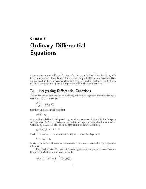
Chapter7Ordinary Differential EquationsMatlab has several different functions for the numerical solution of ordinary dif-ferential equations.This chapter describes the simplest of these functions and then compares all of the functions for efficiency,accuracy,and special features.Stiffness is a subtle concept that plays an important role in these comparisons.7.1Integrating Differential EquationsThe initial value problem for an ordinary differential equation involvesfinding a function y(t)that satisfiesdy(t)=f(t,y(t))dttogether with the initial conditiony(t0)=y0A numerical solution to this problem generates a sequence of values for the indepen-dent variable,t0,t1,...,and a corresponding sequence of values for the dependent variable,y0,y1,...,so that each y n approximates the solution at t n y n≈y(t n),n=0,1,...Modern numerical methods automatically determine the step sizesh n=t n+1−t nso that the estimated error in the numerical solution is controlled by a specified tolerance.The Fundamental Theorem of Calculus gives us an important connection be-tween differential equations and integrals.t+hy(t+h)=y(t)+f(s,y(s))dst12Chapter7.Ordinary Differential Equations We cannot use numerical quadrature directly to approximate the integral because we do not know the function y(s)and so cannot evaluate the integrand.Nevertheless, the basic idea is to choose a sequence of values of h so that this formula allows us to generate our numerical solution.One special case to keep in mind is the situation where f(t,y)is a function of t alone.The numerical solution of such simple differential equations is then just a sequence of quadratures.y n+1=y n+ tn+1t nf(s)dsThrough this chapter,we frequently use“dot”notation for derivatives,˙y=dy(t)dtand¨y=d2y(t)dt27.2Systems of EquationsMany mathematical models involve more than one unknown function,and second and higher order derivatives.These models can be handled by making y(t)a vector-valued function of t.Each component is either one of the unknown functions or one of its derivatives.The Matlab vector notation is particularly convenient here.For example,the second-order differential equation describing a simple har-monic oscillator¨x(t)=−x(t)becomes twofirst-order equations.The vector y(t)has two components,x(t)and itsfirst derivative˙x(t),y(t)=x(t)˙x(t)Using this vector,the differential equation is˙y(t)=˙x(t)−x(t)=y2(t)−y1(t)The Matlab function defining the differential equation has t and y as input arguments and should return f(t,y)as a column vector.For the harmonic oscillator, the function isfunction ydot=harmonic(t,y)ydot=[y(2);-y(1)]A fancier version uses matrix multiplication in an inline function.f=inline(’[01;-10]*y’,’t’,’y’);7.3.Linearized Differential Equations3 In both cases,the variable t has to be included as thefirst argument,even though it is not explicitly involved in the differential equation.A slightly more complicated example,the two-body problem,describes the orbit of one body under the gravitational attraction of a much heavier ing Cartesian coordinates,u(t)and v(t),centered in the heavy body,the equations are ¨u(t)=−u(t)/r(t)3¨v(t)=−v(t)/r(t)3wherer(t)=u(t)+v(t)The vector y(t)has four components,y(t)=u(t)v(t)˙u(t)˙v(t)The differential equation is˙y(t)=˙u(t)˙v(t)−u(t)/r(t)3−v(t)/r(t)3The Matlab function could befunction ydot=twobody(t,y)r=sqrt(y(1)^2+y(2)^2);ydot=[y(3);y(4);-y(1)/r^3;-y(2)/r^3];A more compact Matlab function isfunction ydot=twobody(t,y)ydot=[y(3:4);-y(1:2)/norm(y(1:2))^3]Despite the use of vector operations,the second M-file is not significantly more efficient than thefirst.7.3Linearized Differential EquationsThe local behavior of the solution to a differential equation near any point(t c,y c) can be analyzed by expanding f(t,y)in a two-dimensional Taylor series.f(t,y)=f(t c,y c)+α(t−t c)+J(y−y c)+...whereα=∂f∂t(t c,y c),J=∂f∂y(t c,y c)4Chapter7.Ordinary Differential Equations The most important term in this series is usually the one involving J,the Jacobian. For a system of differential equations with n components,d dty1(t)y2(t)...y n(t)=f1(t,y1,...,y n)f2(t,y1,...,y n)...f n(t,y1,...,y n)the Jacobian is an n-by-n matrix of partial derivativesJ=∂f1∂y1∂f1∂y2...∂f1∂y n ∂f2∂y1∂f2∂y2...∂f2∂y n.........∂f n∂y1∂f n∂y2...∂f n∂y nThe influence of the Jacobian on the local behavior is determined by the solution to the linear system of ordinary differential equations˙y=JyLetλk=µk+iνk be the eigenvalues of J andΛ=diag(λk)the diagonal eigenvalue matrix.If there is a linearly independent set of corresponding eigenvectors V,then J=VΛV−1The linear transformationV x=ytransforms the local system of equations into a set of decoupled equations for the individual components of x,˙x k=λk x kThe solutions arex k(t)=eλk(t−t c)x(t c)A single component x k(t)grows with t ifµk is positive,decays ifµk is negative, and oscillates ifνk is nonzero.The components of the local solution y(t)are linear combinations of these behaviors.For example the harmonic oscillator˙y=01−10yis a linear system.The Jacobian is simply the matrixJ=01−107.4.Single-Step Methods 5The eigenvalues of J are ±i and the solutions are purely oscillatory linear combi-nations of e it and e −it .A nonlinear example is the two-body problem ˙y (t )= y 3(t )y 4(t )−y 1(t )/r (t )3−y 2(t )/r (t )3wherer (t )= y 1(t )2+y 2(t )2In an exercise,we ask you to show that the Jacobian for this system is J =1r 5 00r 50000r 52y 21−y 223y 1y 2003y 1y 22y 22−y 2100It turns out that the eigenvalues of J just depend on the radius r (t )λ=1r3/2 √2i −√2−iWe see that one eigenvalue is real and positive,so the corresponding component of the solution is growing.One eigenvalue is real and negative,corresponding to a decaying component.Two eigenvalues are purely imaginary,corresponding to os-cillatory components.However,the overall global behavior of this nonlinear system is quite complicated,and is not described by this local linearized analysis.7.4Single-Step MethodsThe simplest numerical method for the solution of initial value problems is Euler’s method.It uses a fixed step size h and generates the approximate solution byy n +1=y n +hf (t n ,y n )t n +1=t n +hThe Matlab code would use an initial point t0,a final point tfinal ,an initial value y0,a step size h ,and an inline function or function handle f .The primary loop would simply bet =t0;y =y0;while t <=tfinaly =y +h*feval(f,t,y)t =t +hend6Chapter7.Ordinary Differential Equations Note that this works perfectly well if y0is a vector and f returns a vector.As a quadrature rule for integrating f(t),Euler’s method corresponds to a rectangle rule where the integrand is evaluated only once,at the left hand endpoint of the interval.It is exact if f(t)is constant,but not if f(t)is linear.So the error is proportional to h.Tiny steps are needed to get even a few digits of accuracy. But,from our point of view,the biggest defect of Euler’s method is that it does not provide an error estimate.There is no automatic way to determine what step size is needed to achieve a specified accuracy.If Euler’s method is followed by a second function evaluation,we begin to get a viable algorithm.There are two natural possibilities,corresponding to the midpoint rule and the trapezoid rule for quadrature.The midpoint analog uses Euler to step halfway across the interval,evaluates the function at this intermediate point,then uses that slope to take the actual step.s1=f(t n,y n)s2=f(t n+h2,y n+h2s1)y n+1=y n+hs2t n+1=t n+hThe trapezoid analog uses Euler to take a tentative step across the interval,evaluates the function at this exploratory point,then averages the two slopes to take the actual step.s1=f(t n,y n)s2=f(t n+h,y n+hs1)y n+1=y n+h s1+s22t n+1=t n+hIf we were to use both of these methods simultaneously,they would produce two different values for y n+1.The difference between the two values would provide an error estimate and a basis for picking the step size.Furthermore,an extrapolated combination of the two values would be more accurate than either one individually.Continuing with this approach is the idea behind single-step methods for inte-grating ODEs.The function f(t,y)is evaluated several times for values of t between t n and t n+1and values of y obtained by adding linear combinations of the values of f to y n.The actual step is taken using another linear combination of the function values.Modern versions of single-step methods use yet another linear combination of function values to estimate error and determine step size.Single-step methods are often called Runge-Kutta methods,after the two Ger-man applied mathematicians whofirst wrote about them around1905.The classical Runge-Kutta method was widely used for hand computation before the invention of digital computers and is still popular today.It uses four function evaluations per step.s1=f(t n,y n)7.4.Single-Step Methods7s2=f(t n+h2,y n+h2s1)s3=f(t n+h2,y n+h2s2)s4=f(t n+h,y n+hs3)y n+1=y n+h6(s1+2s2+2s3+s4)t n+1=t n+hIf f(t,y)does not depend on y,then classical Runge-Kutta has s2=s3and the method reduces to Simpson’s quadrature rule.Classical Runge-Kutta does not provide an error estimate.The method is sometimes used with a step size h and again with step size h/2to obtain an error estimate,but we now know more efficient methods.Several of the ODE solvers in Matlab,including the textbook solver we describe later in this chapter,are single-step or Runge-Kutta solvers.A general single-step method is characterized by a number of parameters,αi,βi,j,γi,andδi. There are k stages.Each stage computes a slope,s i,by evaluating f(t,y)for a particular value of t and a value of y obtained by taking linear combinations of the previous slopes.s i=f(t n+αi h,y n+h i−1j=1βi,j s j),i=1,...,kThe proposed step is also a linear combination of the slopes.y n+1=y n+hki=1γi s iAn estimate of the error that would occur with this step is provided by yet another linear combination of the slopes.e n+1=hki=1δi s iIf this error is less than the specified tolerance,then the step is successful and y n+1 is accepted.If not,the step is a failure and y n+1is rejected.In either case,the error estimate is used to compute the step size h for the next step.The parameters in these methods are determined by matching terms in Taylor series expansions of the slopes.These series involve powers of h and products of various partial derivatives of f(t,y).The order of a method is the exponent of the smallest power of h that cannot be matched.It turns out that one,two,three,or four stages yield methods of order one,two,three or four,respectively.But it takes six stages to obtain afifth-order method.The classical Runge-Kutta method has four stages and is fourth-order.The names of the Matlab ODE solvers are all of the form odennxx with digits nn indicating the order of the underlying method and a possibly empty xx indicating8Chapter7.Ordinary Differential Equationssome special characteristic of the method.If the error estimate is obtained by comparing formulas with different orders,the digits nn indicate these orders.For example,ode45obtains its error estimate by comparing a fourth-order and afifth-order formula.7.5The BS23AlgorithmOur textbook function ode23tx is a simplified version of the function ode23that is included with Matlab.The algorithm is due to Bogacki and Shampine[3,6].The “23”in the function names indicates that two simultaneous single step formulas, one of second order and one of third order,are involved.The method has three stages,but there are four slopes s i because,after the first step,the s1for one step is the s4from the previous step.The essentials are s1=f(t n,y n)s2=f(t n+h2,y n+h2s1)s3=f(t n+34h,y n+34hs2)t n+1=t n+hy n+1=y n+h9(2s1+3s2+4s3)s4=f(t n+1,y n+1)e n+1=h72(−5s1+6s2+8s3−9s4)The simplified pictures infigure7.1show the starting situation and the three stages.We start at a point(t n,y n)with an initial slope s1=f(t n,y n)and an estimate of a good step size,h.Our goal is to compute an approximate solution y n+1at t n+1=t n+h that agrees with true solution y(t n+1)to within the specified tolerances.Thefirst stage uses the initial slope s1to take an Euler step halfway across the interval.The function is evaluated there to get the second slope,s2.This slope is used to take an Euler step three quarters of the way across the interval.The function is evaluated again to get the third slope,s3.A weighted average of the three slopess=19(2s1+3s2+4s3)is used for thefinal step all the way across the interval to get a tentative value for y n+1.The function is evaluated once more to get s4.The error estimate then uses all four slopes.e n+1=h72(−5s1+6s2+8s3−9s4)If the error is within the specified tolerance,then the step is successful,the tentative value of y n+1is accepted,and s4becomes the s1of the next step.If the error isFigure7.1.BS23algorithmtoo large,then the tentative y n+1is rejected and the step must be redone.In either case,the error estimate e n+1provides the basis for determining the step size h for the next step.Thefirst input argument of ode23tx specifies the function f(t,y).This argu-ment can take any of three different forms:•A character string involving t and/or y•An inline function•A function handleThe inline function or the M-file should accept two arguments,usually,but not necessarily,t and y.The result of evaluating the character string or the function should be a column vector containing the values of the derivatives,dy/dt.The second input argument of ode23tx is a vector,tspan,with two compo-nents,t0and tfinal.The integration is carried out over the interval t0≤t≤t finalOne of the simplifications in our textbook code is this form of tspan.Other Matlab ODE solvers allow moreflexible specifications of the integration interval.The third input argument is a column vector,y0,providing the initial value of y0=y(t0).The length of y0tells ode23tx the number of differential equations in the system.10Chapter7.Ordinary Differential EquationsA fourth input argument is optional,and can take two different forms.The simplest,and most common,form is a scalar numerical value,rtol,to be used as the relative error tolerance.The default value for rtol is10−3,but you can provide a different value if you want more or less accuracy.The more complicated possibility for this optional argument is the structure generated by the Matlab function odeset.This function takes pairs of arguments that specify many different options for the Matlab ODE solvers.For ode23tx,you can change the default values of three quantities,the relative error tolerance,the absolute error tolerance, and the M-file that is called after each successful step.The statement opts=odeset(’reltol’,1.e-5,’abstol’,1.e-8,...’outputfcn’,@myodeplot)creates a structure that specifies the relative error tolerance to be10−5,the absolute error tolerance to be10−8,and the output function to be myodeplot.The output produced by ode23tx can be either graphic or numeric.With no output arguments,the statementode23tx(F,tspan,y0);produces a dynamic plot of all the components of the solution.With two output arguments,the statement[tout,yout]=ode23tx(F,tspan,y0);generates a table of values of the solution.7.6ode23txLet’s examine the code for ode23tx.Here is the preamble.function[tout,yout]=ode23tx(F,tspan,y0,arg4,varargin)%ODE23TX Solve non-stiff differential equations.%Textbook version of ODE23.%%ODE23TX(F,TSPAN,Y0)with TSPAN=[T0TFINAL]integrates%the system of differential equations y’=f(t,y)from%t=T0to t=TFINAL.The initial condition is%y(T0)=Y0.The input argument F is the name of an%M-file,or an inline function,or simply a character%string,defining f(t,y).This function must have two%input arguments,t and y,and must return a column vector%of the derivatives,y’.%%With two output arguments,[T,Y]=ODE23TX(...)returns%a column vector T and an array Y where Y(:,k)is the%solution at T(k).%7.6.ode23tx11%With no output arguments,ODE23TX plots the solution.%%ODE23TX(F,TSPAN,Y0,RTOL)uses the relative error%tolerance RTOL instead of the default 1.e-3.%%ODE23TX(F,TSPAN,Y0,OPTS)where OPTS=ODESET(’reltol’,...%RTOL,’abstol’,ATOL,’outputfcn’,@PLTFN)uses relative error %RTOL instead of 1.e-3,absolute error ATOL instead of% 1.e-6,and calls PLTFN instead of ODEPLOT after each step.%%More than four input arguments,ODE23TX(F,TSPAN,Y0,RTOL,%P1,P2,..),are passed on to F,F(T,Y,P1,P2,..).%%ODE23TX uses the Runge-Kutta(2,3)method of Bogacki and%Shampine.%%Example%tspan=[02*pi];%y0=[10]’;%F=’[01;-10]*y’;%ode23tx(F,tspan,y0);%%See also ODE23.Here is the code that parses the arguments and initializes the internal variables.rtol= 1.e-3;atol= 1.e-6;plotfun=@odeplot;if nargin>=4&isnumeric(arg4)rtol=arg4;elseif nargin>=4&isstruct(arg4)if~isempty(arg4.RelTol),rtol=arg4.RelTol;endif~isempty(arg4.AbsTol),atol=arg4.AbsTol;endif~isempty(arg4.OutputFcn),plotfun=arg4.OutputFcn;end endt0=tspan(1);tfinal=tspan(2);tdir=sign(tfinal-t0);plotit=(nargout==0);threshold=atol/rtol;hmax=abs(0.1*(tfinal-t0));t=t0;y=y0(:);%Make F callable by feval.12Chapter7.Ordinary Differential Equations if ischar(F)&exist(F)~=2F=inline(F,’t’,’y’);elseif isa(F,’sym’)F=inline(char(F),’t’,’y’);end%Initialize output.if plotitfeval(plotfun,tspan,y,’init’);elsetout=t;yout=y.’;endThe computation of the initial step size is a delicate matter because it requires some knowledge of the overall scale of the problem.s1=feval(F,t,y,varargin{:});r=norm(s1./max(abs(y),threshold),inf)+realmin;h=tdir*0.8*rtol^(1/3)/r;Here is the beginning of the main loop.The integration starts at t=t0and increments t until it reaches t final.It is possible to go“backward,”that is,have t final<t0.while t~=tfinalhmin=16*eps*abs(t);if abs(h)>hmax,h=tdir*hmax;endif abs(h)<hmin,h=tdir*hmin;end%Stretch the step if t is close to tfinal.if 1.1*abs(h)>=abs(tfinal-t)h=tfinal-t;endHere is the actual computation.Thefirst slope s1has already been computed.The function defining the differential equation is evaluated three more times to obtain three more slopes.s2=feval(F,t+h/2,y+h/2*s1,varargin{:});s3=feval(F,t+3*h/4,y+3*h/4*s2,varargin{:});tnew=t+h;ynew=y+h*(2*s1+3*s2+4*s3)/9;s4=feval(F,tnew,ynew,varargin{:});7.6.ode23tx13 Here is the error estimate.The norm of the error vector is scaled by the ratio of the absolute tolerance to the relative tolerance.The use of the smallestfloating-point number,realmin,prevents err from being exactly zero.e=h*(-5*s1+6*s2+8*s3-9*s4)/72;err=norm(e./max(max(abs(y),abs(ynew)),threshold),...inf)+realmin;Here is the test to see if the step is successful.If it is,the result is plotted or appended to the output vector.If it is not,the result is simply forgotten.if err<=rtolt=tnew;y=ynew;if plotitif feval(plotfun,t,y,’’);breakendelsetout(end+1,1)=t;yout(end+1,:)=y.’;ends1=s4;%Reuse final function value to start new step.endThe error estimate is used to compute a new step size.The ratio rtol/err is greater than one if the current step is successful,or less than one if the current step fails.A cube root is involved because the BS23is a third-order method.This means that changing tolerances by a factor of eight will change the typical step size,and hence the total number of steps,by a factor of two.The factors0.8and5prevent excessive changes in step size.%Compute a new step size.h=h*min(5,0.8*(rtol/err)^(1/3));Here is the only place where a singularity would be detected.if abs(h)<=hminwarning(sprintf(...’Step size%e too small at t=%e.\n’,h,t));t=tfinal;endendThat ends the main loop.The plot function might need tofinish its work.if plotitfeval(plotfun,[],[],’done’);end14Chapter7.Ordinary Differential Equations 7.7ExamplesPlease sit down in front of a computer running Matlab.Make sure ode23tx is in your current directory or on your Matlab path.Start your session by entering ode23tx(’0’,[010],1)This should produce a plot of the solution of the initial value problem dy=0dty(0)=10≤t≤10The solution,of course,is a constant function,y(t)=1.Now you can press the up arrow key,use the left arrow key to space over to the’0’,and change it to something more interesting.Here are some examples.At first,we’ll change just the’0’and leave the[010]and1alone.F Exact solution’0’1’t’1+t^2/2’y’exp(t)’-y’exp(-t)’1/(1-3*t)’1-log(1-3*t)/3(Singular)’2*y-y^2’2/(1+exp(-2*t))Make up some of your own examples.Change the initial condition.Change the accuracy by including1.e-6as the fourth argument.Now let’s try the harmonic oscillator,a second-order differential equation writ-ten as a pair of twofirst-order equations.First,create an inline function to specify the e eitherF=inline(’[y(2);-y(1)]’,’t’,’y’)orF=inline(’[01;-10]*y’,’t’,’y’)Then,the statementode23tx(F,[02*pi],[1;0])plots two functions of t that you should recognize.If you want to produce a phase plane plot,you have two choices.One possibility is to capture the output and plot it after the computation is complete.[t,y]=ode23tx(F,[02*pi],[1;0])plot(y(:,1),y(:,2),’-o’)axis([-1.2 1.2-1.2 1.2])axis square7.7.Examples15The more interesting possibility is to use a function that plots the solution while it is being computed.Matlab provides such a function in odephas2.m.It is accessed by using odeset to create an options structureopts=odeset(’reltol’,1.e-4,’abstol’,1.e-6,...’outputfcn’,@odephas2);If you want to provide your own plotting function,it should be something like function flag=phaseplot(t,y,job)persistent pif isequal(job,’init’)p=plot(y(1),y(2),’o’,’erasemode’,’none’);axis([-1.21.2-1.2 1.2])axis squareflag=0;elseif isequal(job,’’)set(p,’xdata’,y(1),’ydata’,y(2))drawnowflag=0;endThis is withopts=odeset(’reltol’,1.e-4,’abstol’,1.e-6,...’outputfcn’,@phaseplot);Once you have decided on a plotting function and created an options structure,you can compute and simultaneously plot the solution withode23tx(F,[02*pi],[1;0],opts)Try this with other values of the tolerances.Issue the command type twobody to see if there is an M-file twobody.m on your path.If not,find the three lines of code earlier in this chapter and create your own M-file.Then tryode23tx(@twobody,[02*pi],[1;0;0;1]);The code,and the length of the initial condition,indicate that the solution has four components.But the plot shows only three.Why?Hint:find the zoom button on thefigure window toolbar and zoom in on the blue curve.You can vary the initial condition of the two-body problem by changing the fourth component.y0=[1;0;0;change_this];ode23tx(@twobody,[02*pi],y0);Graph the orbit,and the heavy body at the origin,with16Chapter7.Ordinary Differential Equations y0=[1;0;0;change_this];[t,y]=ode23tx(@twobody,[02*pi],y0);plot(y(:,1),y(:,2),’-’,0,0,’ro’)axis equalYou might also want to use something other than2πfor tfinal.7.8Lorenz AttractorOne of the world’s most extensively studied ordinary differential equations is the Lorenz chaotic attractor.It wasfirst described in1963by Edward Lorenz,an MIT mathematician and meteorologist,who was interested influidflow models of the earth’s atmosphere.An excellent reference is a book by Colin Sparrow[8].We have chosen to express the Lorenz equations in a somewhat unusual way, involving a matrix-vector product.˙y=AyThe vector y has three components that are functions of t,y(t)=y1(t)y2(t)y3(t)Despite the way we have written it,this is not a linear system of differential equa-tions.Seven of the nine elements in the3-by-3matrix A are constant,but the other two depend on y2(t).A=−β0y20−σσ−y2ρ−1Thefirst component of the solution,y1(t),is related to the convection in the atmo-sphericflow,while the other two components are related to horizontal and vertical temperature variation.The parameterσis the Prandtl number,ρis the normal-ized Rayleigh number,andβdepends on the geometry of the domain.The most popular values of the parameters,σ=10,ρ=28,andβ=8/3,are outside the ranges associated with the earth’s atmosphere.The deceptively simple nonlinearity introduced by the presence of y2in the system matrix A changes everything.There are no random aspects to these equa-tions,so the solutions y(t)are completely determined by the parameters and the initial conditions,but their behavior is very difficult to predict.For some values of the parameters,the orbit of y(t)in three-dimensional space is known as a strange attractor.It is bounded,but not periodic and not convergent.It never intersects itself.It ranges chaotically back and forth around two different points,or attractors. For other values of the parameters,the solution might converge to afixed point, diverge to infinity,or oscillate periodically.Figure 7.2.Three components of LorenzattractorFigure 7.3.Phase plane plot of Lorenz attractorLet’s think of η=y 2as a free parameter,restrict ρto be greater than one,and study the matrixA = −β0η0−σσ−ηρ−1It turns out that A is singular if and only if η=±β(ρ−1)18Chapter 7.Ordinary Differential EquationsThe corresponding null vector,normalized so that its second component is equal to η,isρ−1ηηWith two different signs for η,this defines two points in three-dimensional space.These points are fixed points for the differential equation.Ify (t 0)= ρ−1ηηthen,for all t ,˙y (t )=00and so y (t )never changes.However,these points are unstable fixed points.If y (t )does not start at one of these points,it will never reach either of them;if it tries to approach either point,it will be repulsed.We have provided an M-file,lorenzgui.m ,that facilitates experiments with the Lorenz equations.Two of the parameters,β=8/3and σ=10,are fixed.A uicontrol offers a choice among several different values of the third parameter,ρ.A simplified version of the program for ρ=28would begin withrho =28;sigma =10;beta =8/3;eta =sqrt(beta*(rho-1));A =[-beta 0eta0-sigma sigma -eta rho -1];The initial condition is taken to be near one of the attractors.yc =[rho-1;eta;eta];y0=yc +[0;0;3];The time span is infinite,so the integration will have to be stopped by another uicontrol .tspan =[0Inf];opts =odeset(’reltol’,1.e-6,’outputfcn’,@lorenzplot);ode45(@lorenzeqn,tspan,y0,opts,A);The matrix A is passed as an extra parameter to the integrator,which sends it on to lorenzeqn ,the subfunction defining the differential equation.The extra parameter machinery included in the function functions allows lorenzeqn to be written in a particularly compact manner.。

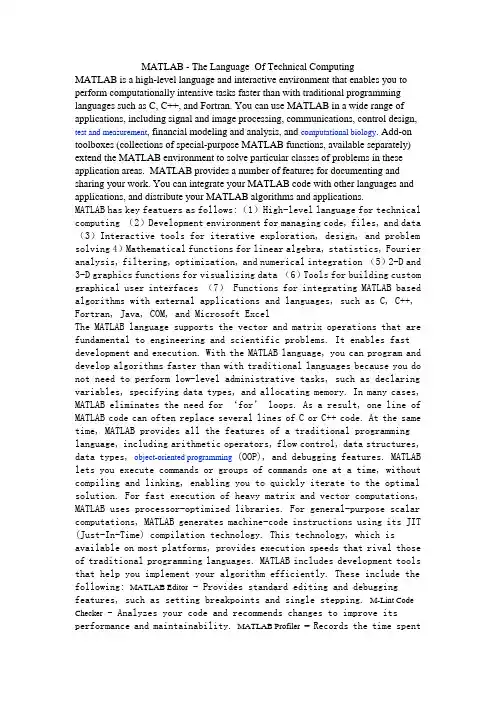
MATLAB - The Language Of Technical ComputingMATLAB is a high-level language and interactive environment that enables you to perform computationally intensive tasks faster than with traditional programming languages such as C, C++, and Fortran. You can use MATLAB in a wide range of applications, including signal and image processing, communications, control design, test and measurement, financial modeling and analysis, and computational biology. Add-on toolboxes (collections of special-purpose MATLAB functions, available separately) extend the MATLAB environment to solve particular classes of problems in these application areas.MATLAB provides a number of features for documenting and sharing your work. You can integrate your MATLAB code with other languages and applications, and distribute your MATLAB algorithms and applications.MATLAB has key featuers as follows:（1）High-level language for technical computing （2）Development environment for managing code, files, and data （3）Interactive tools for iterative exploration, design, and problem solving 4）Mathematical functions for linear algebra, statistics, Fourier analysis, filtering, optimization, and numerical integration （5）2-D and 3-D graphics functions for visualizing data （6）Tools for building custom graphical user interfaces （7） Functions for integrating MATLAB based algorithms with external applications and languages, such as C, C++, Fortran, Java, COM, and Microsoft ExcelThe MATLAB language supports the vector and matrix operations that are fundamental to engineering and scientific problems. It enables fast development and execution. With the MATLAB language, you can program and develop algorithms faster than with traditional languages because you do not need to perform low-level administrative tasks, such as declaring variables, specifying data types, and allocating memory. In many cases, MATLAB eliminates the need for ‘for’ loops. As a result, one line of MATLAB code can often replace several lines of C or C++ code. At the same time, MATLAB provides all the features of a traditional programming language, including arithmetic operators, flow control, data structures, data types, object-oriented programming (OOP), and debugging features. MATLAB lets you execute commands or groups of commands one at a time, without compiling and linking, enabling you to quickly iterate to the optimal solution. For fast execution of heavy matrix and vector computations, MATLAB uses processor-optimized libraries. For general-purpose scalar computations, MATLAB generates machine-code instructions using its JIT (Just-In-Time) compilation technology. This technology, which is available on most platforms, provides execution speeds that rival those of traditional programming languages. MATLAB includes development tools that help you implement your algorithm efficiently. These include the following: MATLAB Editor - Provides standard editing and debugging features, such as setting breakpoints and single stepping. M-Lint Code Checker - Analyzes your code and recommends changes to improve its performance and maintainability. MATLAB Profiler - Records the time spentexecuting each line of code. Directory Reports- Scan all the files in a directory and report on code efficiency, file differences, file dependencies, and code coverage。

一、Matlab在因式分解中的应用Matlab作为一种高级的数学计算软件，具有强大的因式分解功能。

在数学中，因式分解是将一个多项式分解成若干个一次或多次多项式的乘积的过程。

Matlab通过简单的几行代码就可以实现多项式的因式分解，极大地方便了数学计算和解题过程。

在Matlab中，通过使用“factor”函数可以对多项式进行因式分解。

如果有一个多项式为p(x) = x^2 - 4，那么在Matlab中可以使用以下代码进行因式分解：```syms xp = x^2 - 4;factors = factor(p);```这段代码就可以得到p(x)的因式分解结果factors = (x-2)*(x+2)，从而简单地实现了多项式的因式分解。

二、Matlab在微分方程中的应用微分方程是描述自然界中各种现象的最基本的数学模型之一，而在求解微分方程的过程中，Matlab也可以发挥其强大的计算能力。

通过Matlab中的“dsolve”函数，可以对各种类型的微分方程进行求解，无论是常微分方程还是偏微分方程。

以一阶常微分方程为例，对于方程dy/dx = x^2，可以使用以下代码在Matlab中进行求解：```syms y(x)eqn = diff(y,x) == x^2;cond = y(0) == 1;ySol(x) = dsolve(eqn,cond);```这段代码中，首先定义了微分方程dy/dx = x^2和初始条件y(0) = 1，然后通过“dsolve”函数求解得到了微分方程的解ySol(x)。

而对于更为复杂的高阶微分方程或者偏微分方程，Matlab同样可以提供便捷的求解方法，极大地简化了数学建模和科学计算的过程。

总结作为一种专业的数学计算软件，Matlab在因式分解和微分方程求解中都具有强大的功能和性能。

通过简单的几行代码，就可以实现复杂多项式的因式分解以及各种类型微分方程的求解，极大地提高了数学建模和科学计算的效率。

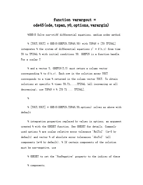
function varargout =ode45(ode,tspan,y0,options,varargin)%ODE45 Solve non-stiff differential equations, medium order method.% [TOUT,YOUT] = ODE45(ODEFUN,TSPAN,Y0) with TSPAN = [T0 TFINAL] integrates % the system of differential equations y' = f(t,y) from time T0 to TFINAL % with initial conditions Y0. ODEFUN is a function handle. For a scalar T% and a vector Y, ODEFUN(T,Y) must return a column vector corresponding % to f(t,y). Each row in the solution array YOUT corresponds to a time % returned in the column vector TOUT. To obtain solutions at specific % times T0,T1,...,TFINAL (all increasing or all decreasing), use TSPAN = % [T0 T1 ... TFINAL].%% [TOUT,YOUT] = ODE45(ODEFUN,TSPAN,Y0,options) solves as above with default% integration properties replaced by values in options, an argument created % with the ODESET function. See ODESET for details. Commonly used options % are scalar relative error tolerance 'RelTol' (1e-3 by default) and vector % of absolute error tolerances 'AbsTol' (all components 1e-6 by default). % If certain components of the solution must be non-negative, use% ODESET to set the 'NonNegative' property to the indices of these% components.%% ODE45 can solve problems M(t,y)*y' = f(t,y) with mass matrix Mthat is % nonsingular. Use ODESET to set the 'Mass' property to afunction handle % MASS if MASS(T,Y) returns the value of the mass matrix. If the mass matrix % is constant, the matrix can be used as the value of the 'Mass' option. If% the mass matrix does not depend on the state variable Y and the function % MASS is to be called with one input argument T, set'MStateDependence' to% 'none'. ODE15S and ODE23T can solve problems with singular mass matrices. %% [TOUT,YOUT,TE,YE,IE] = ODE45(ODEFUN,TSPAN,Y0,OPTIONS) with the'Events' % property in OPTIONS set to a function handle EVENTS, solvesas above % while also finding where functions of (T,Y), called event functions, % are zero. For each function you specify whether the integration is% to terminate at a zero and whether the direction of the zero crossing % matters. These are the three column vectors returned by EVENTS:% [VALUE,ISTERminAL,DIRECTION] = EVENTS(T,Y). For the I-th event function: % VALUE(I) is the value of the function, ISTERminAL(I)=1 ifthe integration % is to terminate at a zero of this event function and 0 otherwise.% DIRECTION(I)=0 if all zeros are to be computed (the default), +1 if only % zeros where the event function is increasing, and -1 if only zeros where % the event function is decreasing. output TE is a column vector of times % at which events occur. Rows of YE are the corresponding solutions, and % indices in vector IE specify which event occurred.%% SOL = ODE45(ODEFUN,[T0 TFINAL],Y0...) returns a structure that can be % used with DEVAL to evaluate the solution or its first derivative at% any point between T0 and TFINAL. The steps chosen by ODE45 are returned % in a row vector SOL.x. For each I, the column SOL.y(:,I) contains% the solution at SOL.x(I). If events were detected, SOL.xe is a row vector % of points at which events occurred. Columns of SOL.ye are the corresponding% solutions, and indices in vector SOL.ie specify which event occurred. %% Example% [t,y]=ode45(@vdp1,[0 20],[2 0]);% plot(t,y(:,1));% solves the system y' = vdp1(t,y), using the default relativeerror % tolerance 1e-3 and the default absolute tolerance of 1e-6 for each % component, and plots the first component of the solution.%% Class support for inputs TSPAN, Y0, and the result of ODEFUN(T,Y):% float: double, single%% See also% other ODE solvers: ODE23, ODE113, ODE15S, ODE23S, ODE23T, ODE23TB% implicit ODEs: ODE15I% options handling: ODESET, ODEGET% output functions: ODEPLOT, ODEPHAS2, ODEPHAS3, ODEPRINT% evaluating solution: DEVAL% ODE examples: RIGIDODE, BALLODE, ORBITODE% function handles: function_HANDLE%% NOTE:% The interpretation of the first input argument of the ODE solvers and % some properties available through ODESET have changed in MATLAB6.0. % Although we still support the v5 syntax, any new functionality is % available only with the new syntax. To see the v5 help, type in% the command line% more on, type ode45, more off% NOTE:% This portion describes the v5 syntax of ODE45.%% [T,Y] = ODE45('F',TSPAN,Y0) with TSPAN = [T0 TFINAL] integrates the% system of differential equations y' = F(t,y) from time T0 to TFINAL with % initial conditions Y0. 'F' is a string containing the name of an ODE % file. Function F(T,Y) must return a column vector. Each row in% solution array Y corresponds to a time returned in column vector T. To % obtain solutions at specific times T0, T1, ..., TFINAL (all increasing % or all decreasing), use TSPAN = [T0 T1 ... TFINAL].%% [T,Y] = ODE45('F',TSPAN,Y0,options) solves as above with default% integration parameters replaced by values in options, an argument% created with the ODESET function. See ODESET for details. Commonly% used options are scalar relative error tolerance 'RelTol' (1e-3 by% default) and vector of absolute error tolerances 'AbsTol' (all% components 1e-6 by default).%% [T,Y] = ODE45('F',TSPAN,Y0,OPTIONS,P1,P2,...) passes the additional% parameters P1,P2,... to the ODE file as F(T,Y,FLAG,P1,P2,...) (see% ODEFILE). Use OPTIONS = [] as a place holder if no options are set. %% It is possible to specify TSPAN, Y0 and OPTIONS in the ODE file (see % ODEFILE). If TSPAN or Y0 is empty, then ODE45 calls the ODE file% [TSPAN,Y0,OPTIONS] = F([],[],'init') to obtain any values not supplied % in the ODE45 argument list. Empty arguments at the end of the call list % may be omitted, e.g. ODE45('F').%% ODE45 can solve problems M(t,y)*y' = F(t,y) with a mass matrix M that is% nonsingular. Use ODESET to set Mass to 'M', 'M(t)', or 'M(t,y)' if the% ODE file is coded so that F(T,Y,'mass') returns a constant,% time-dependent, or time- and state-dependent mass matrix, respectively. % The default value of Mass is 'none'. ODE15S and ODE23T can solve problems % with singular mass matrices.%% [T,Y,TE,YE,IE] = ODE45('F',TSPAN,Y0,options) with the Events property in% options set to 'on', solves as above while also locating zero crossings % of an event function defined in the ODE file. The ODE file must be% coded so that F(T,Y,'events') returns appropriate information. See% ODEFILE for details. output TE is a column vector of times at which % events occur, rows of YE are the corresponding solutions, and indices in% vector IE specify which event occurred.%% See also ODEFILE% ODE45 is an implementation of the explicit Runge-Kutta (4,5) pair of % Dormand and Prince called variously RK5(4)7FM, DOPRI5, DP(4,5) and DP54. % It uses a "free" interpolant of order 4 communicated privatelyby% Dormand and Prince. Local extrapolation is done.% Details are to be found in The MATLAB ODE Suite, L. F. Shampine and% M. W. Reichelt, SIAM Journal on Scientific Computing, 18-1, 1997.% Mark W. Reichelt and Lawrence F. Shampine, 6-14-94% Copyright 1984-2009 The MathWorks, Inc.% $Revision: 5.74.4.10 $ $Date: 2009/04/21 03:24:15 $solver_name = 'ode45';% Check inputsif nargin < 4options = [];if nargin < 3y0 = [];if nargin < 2tspan = [];if nargin < 1error('MATLAB:ode45:NotEnoughInputs',...'Not enough input arguments. See ODE45.');endendendend% Statsnsteps = 0;nfailed = 0;nfevals = 0;% outputFcnHandlesUsed = isa(ode,'function_handle');output_sol = (FcnHandlesUsed && (nargout==1)); % sol = odeXX(...) output_ty = (~output_sol && (nargout > 0)); % [t,y,...] = odeXX(...)% There might be no output requested...sol = []; f3d = [];if output_solsol.solver = solver_name;sol.extdata.odefun = ode;sol.extdata.options = options;sol.extdata.varargin = varargin;end% Handle solver arguments[neq, tspan, ntspan, next, t0, tfinal, tdir, y0, f0, odeArgs, odeFcn, ... options, threshold, rtol, normcontrol, normy, hmax, htry, htspan, dataType] = ...odearguments(FcnHandlesUsed, solver_name, ode, tspan, y0, options, varargin);nfevals = nfevals + 1;% Handle the outputif nargout > 0outputFcn = odeget(options,'OutputFcn',[],'fast');elseoutputFcn = odeget(options,'OutputFcn',@odeplot,'fast');endoutputArgs = {};if isempty(outputFcn)haveOutputFcn = false;elsehaveOutputFcn = true;outputs = odeget(options,'OutputSel',1:neq,'fast');if isa(outputFcn,'function_handle')% With MATLAB 6 syntax pass additional input arguments to outputFcn. outputArgs = varargin;endendrefine = max(1,odeget(options,'refine',4,'fast'));if ntspan > 2outputAt = 'RequestedPoints'; % output only at tspan pointselseif refine <= 1outputAt = 'SolverSteps'; % computed points, no refinement elseoutputAt = 'RefinedSteps'; % computed points, with refinement S = (1:refine-1) / refine;endprintstats = strcmp(odeget(options,'Stats','off','fast'),'on');% Handle the event function[haveEventFcn,eventFcn,eventArgs,valt,teout,yeout,ieout] = ...odeevents(FcnHandlesUsed,odeFcn,t0,y0,options,varargin);% Handle the mass matrix[Mtype, M, Mfun] =odemass(FcnHandlesUsed,odeFcn,t0,y0,options,varargin); if Mtype > 0 % non-trivial mass matrixMsingular = odeget(options,'MassSingular','no','fast');if strcmp(Msingular,'maybe')warning('MATLAB:ode45:MassSingularAssumedNo',['ODE45 assumes '...'MassSingular is ''no''. See ODE15S or ODE23T.']);elseif strcmp(Msingular,'yes')error('MATLAB:ode45:MassSingularYes',...['MassSingular cannot be ''yes'' for this solver. See ODE15S '...' or ODE23T.']);end% Incorporate the mass matrix into odeFcn and odeArgs. [odeFcn,odeArgs] =odemassexplicit(FcnHandlesUsed,Mtype,odeFcn,odeArgs,Mfun,M); f0 = feval(odeFcn,t0,y0,odeArgs{:});nfevals = nfevals + 1;end% Non-negative solution componentsidxNonNegative = odeget(options,'NonNegative',[],'fast'); nonNegative = ~isempty(idxNonNegative);if nonNegative % modify the derivative function[odeFcn,thresholdNonNegative] =odenonnegative(odeFcn,y0,threshold,idxNonNegative);f0 = feval(odeFcn,t0,y0,odeArgs{:});nfevals = nfevals + 1;endt = t0;y = y0;% Allocate memory if we're generating output.nout = 0;tout = []; yout = [];if nargout > 0if output_solchunk = min(max(100,50*refine), refine+floor((2^11)/neq)); tout = zeros(1,chunk,dataType);yout = zeros(neq,chunk,dataType);f3d = zeros(neq,7,chunk,dataType);elseif ntspan > 2 % output only at tspan pointstout = zeros(1,ntspan,dataType);yout = zeros(neq,ntspan,dataType);else% alloc in chunkschunk = min(max(100,50*refine), refine+floor((2^13)/neq));tout = zeros(1,chunk,dataType);yout = zeros(neq,chunk,dataType);endendnout = 1;tout(nout) = t;yout(:,nout) = y;end% Initialize method parameters.pow = 1/5;A = [1/5, 3/10, 4/5, 8/9, 1, 1];B = [1/5 3/40 44/45 19372/6561 9017/3168 35/384 0 9/40 -56/15 -25360/2187 -355/33 00 0 32/9 64448/6561 46732/5247 500/11130 0 0 -212/729 49/176 125/1920 0 0 0 -5103/18656 -2187/67840 0 0 0 0 11/840 0 0 0 0 0];E = [71/57600; 0; -71/16695; 71/1920; -17253/339200; 22/525; -1/40];f = zeros(neq,7,dataType);hmin = 16*eps(t);if isempty(htry)% Compute an initial step size h using y'(t).absh = min(hmax, htspan);if normcontrolrh = (norm(f0) / max(normy,threshold)) / (0.8 * rtol^pow);elserh = norm(f0 ./ max(abs(y),threshold),inf) / (0.8 * rtol^pow);endif absh * rh > 1absh = 1 / rh;endabsh = max(absh, hmin);elseabsh = min(hmax, max(hmin, htry));endf(:,1) = f0;% Initialize the output function.if haveoutputFcnfeval(outputFcn,[t tfinal],y(outputs),'init',outputArgs{:});end% THE MAIN LOOPdone = false;while ~done% By default, hmin is a small number such that t+hmin is only slightly % different than t. It might be 0 if t is 0.hmin = 16*eps(t);absh = min(hmax, max(hmin, absh)); % couldn't limit absh until new hmin h = tdir * absh;% Stretch the step if within 10% of tfinal-t.if 1.1*absh >= abs(tfinal - t)h = tfinal - t;absh = abs(h);done = true;end% LOOP FOR ADVANCING ONE STEP.nofailed = true; % no failed attemptswhile truehA = h * A;hB = h * B;f(:,2) = feval(odeFcn,t+hA(1),y+f*hB(:,1),odeArgs{:}); f(:,3) = feval(odeFcn,t+hA(2),y+f*hB(:,2),odeArgs{:}); f(:,4) = feval(odeFcn,t+hA(3),y+f*hB(:,3),odeArgs{:}); f(:,5) = feval(odeFcn,t+hA(4),y+f*hB(:,4),odeArgs{:}); f(:,6) = feval(odeFcn,t+hA(5),y+f*hB(:,5),odeArgs{:}); tnew = t + hA(6);if donetnew = tfinal; % Hit end point exactly.endh = tnew - t; % Purify h.ynew = y + f*hB(:,6);f(:,7) = feval(odeFcn,tnew,ynew,odeArgs{:});nfevals = nfevals + 6;% Estimate the error.NNrejectStep = false;if normcontrolnormynew = norm(ynew);errwt = max(max(normy,normynew),threshold);err = absh * (norm(f * E) / errwt);if nonNegative && (err <= rtol) && any(ynew(idxNonNegative)<0) errNN = norm( max(0,-ynew(idxNonNegative)) ) / errwt ;if errNN > rtolerr = errNN;NNrejectStep = true;endendelseerr = absh * norm((f * E) ./max(max(abs(y),abs(ynew)),threshold),inf);if nonNegative && (err <= rtol) && any(ynew(idxNonNegative)<0)errNN = norm( max(0,-ynew(idxNonNegative)) ./ thresholdNonNegative, inf);if errNN > rtolerr = errNN;NNrejectStep = true;endendend% Accept the solution only if the weighted error is no more than the % tolerance rtol. Estimate an h that will yield an error of rtol on % the next step or the next try at taking this step, as the case may be, % and use 0.8 of this value to avoid failures.if err > rtol % Failed stepnfailed = nfailed + 1;if absh <= hminwarning('MATLAB:ode45:IntegrationTolNotMet',['Failure at t=%e. '... 'Unable to meet integration tolerances without reducing '...'the step size below the smallest value allowed (%e) '...'at time t.'],t,hmin);solver_output = odefinalize(solver_name, sol,...outputFcn, outputArgs,...printstats, [nsteps, nfailed, nfevals],... nout, tout, yout,... haveEventFcn, teout, yeout, ieout,...{f3d,idxNonNegative});if nargout > 0varargout = solver_output;endreturn;endif nofailednofailed = false;if NNrejectStepabsh = max(hmin, 0.5*absh);elseabsh = max(hmin, absh * max(0.1, 0.8*(rtol/err)^pow)); endelseabsh = max(hmin, 0.5 * absh);endh = tdir * absh;done = false;else% Successful stepNNreset_f7 = false;if nonNegative && any(ynew(idxNonNegative)<0)ynew(idxNonNegative) = max(ynew(idxNonNegative),0);if normcontrolnormynew = norm(ynew);endNNreset_f7 = true;endbreak;endendnsteps = nsteps + 1;if haveEventFcn[te,ye,ie,valt,stop] = ...odezero(@ntrp45,eventFcn,eventArgs,valt,t,y,tnew,ynew,t0,h,f,idxNon Nega tive);if ~isempty(te)if output_sol || (nargout > 2)teout = [teout, te];yeout = [yeout, ye];ieout = [ieout, ie];endif stop % Stop on a terminal event.% Adjust the interpolation data to [t te(end)].% Update the derivatives using the interpolating polynomial.taux = t + (te(end) - t)*A;[~,f(:,2:7)] = ntrp45(taux,t,y,[],[],h,f,idxNonNegative);tnew = te(end);ynew = ye(:,end);h = tnew - t;done = true;endendendif output_solnout = nout + 1;if nout > length(tout)tout = [tout, zeros(1,chunk,dataType)]; % requires chunk >= refine yout = [yout, zeros(neq,chunk,dataType)];f3d = cat(3,f3d,zeros(neq,7,chunk,dataType));endtout(nout) = tnew;yout(:,nout) = ynew;f3d(:,:,nout) = f;endif output_ty || haveOutputFcnswitch outputAtcase'SolverSteps'% computed points, no refinementnout_new = 1;tout_new = tnew;yout_new = ynew;case'RefinedSteps'% computed points, with refinementtref = t + (tnew-t)*S;nout_new = refine;tout_new = [tref, tnew];yout_new = [ntrp45(tref,t,y,[],[],h,f,idxNonNegative), ynew];case'RequestedPoints'% output only at tspan points nout_new = 0;tout_new = [];yout_new = [];while next <= ntspanif tdir * (tnew - tspan(next)) < 0if haveEventFcn && stop % output tstop,ystopnout_new = nout_new + 1;tout_new = [tout_new, tnew];yout_new = [yout_new, ynew];endbreak;endnout_new = nout_new + 1;tout_new = [tout_new, tspan(next)];if tspan(next) == tnewyout_new = [yout_new, ynew];elseyout_new = [yout_new,ntrp45(tspan(next),t,y,[],[],h,f,idxNonNegative)];endnext = next + 1;endendif nout_new > 0if output_tyoldnout = nout;nout = nout + nout_new;if nout > length(tout)tout = [tout, zeros(1,chunk,dataType)]; % requires chunk >= refine yout = [yout, zeros(neq,chunk,dataType)];endidx = oldnout+1:nout;tout(idx) = tout_new;yout(:,idx) = yout_new;endif haveoutputFcnstop =feval(outputFcn,tout_new,yout_new(outputs,:),'',outputArgs{:}); if stopdone = true;endendendendif donebreakend% If there were no failures compute a new h.if nofailed% Note that absh may shrink by 0.8, and that err may be 0.temp = 1.25*(err/rtol)^pow;if temp > 0.2absh = absh / temp;elseabsh = 5.0*absh;endend% Advance the integration one step.t = tnew;y = ynew;if normcontrolnormy = normynew;endif NNreset_f7% Used f7 for unperturbed solution to interpolate. % Now reset f7 to move along constraint.f(:,7) = feval(odeFcn,tnew,ynew,odeArgs{:});nfevals = nfevals + 1;endf(:,1) = f(:,7); % Already have f(tnew,ynew)endsolver_output = odefinalize(solver_name, sol,...outputFcn, outputArgs,...printstats, [nsteps, nfailed, nfevals],... nout, tout, yout,... haveEventFcn, teout, yeout, ieout,...{f3d,idxNonNegative});if nargout > 0varargout = solver_output;end。

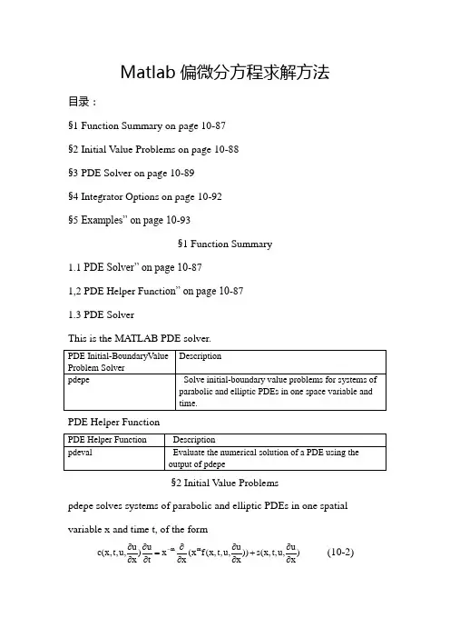
Matlab 偏微分方程求解方法目录：§1 Function Summary on page 10-87§2 Initial Value Problems on page 10-88§3 PDE Solver on page 10-89§4 Integrator Options on page 10-92§5 Examples” on page 10-93§1 Function Summary1.1 PDE Solver” on page 10-871,2 PDE Helper Functi on” on page 10-871.3 PDE SolverThis is the MATLAB PDE solver.PDE Helper Function§2 Initial Value Problemspdepe solves systems of parabolic and elliptic PDEs in one spatial variable x and time t, of the form)xu ,u ,t ,x (s ))x u ,u ,t ,x (f x (x x t u )x u ,u ,t ,x (c m m ∂∂+∂∂∂∂=∂∂∂∂- (10-2) The PDEs hold for b x a ,t t t f 0≤≤≤≤.The interval [a, b] must be finite. mcan be 0, 1, or 2, corresponding to slab, cylindrical, or spherical symmetry,respectively. If m > 0, thena ≥0 must also hold.In Equation 10-2,)x /u ,u ,t ,x (f ∂∂ is a flux term and )x /u ,u ,t ,x (s ∂∂ is a source term. The flux term must depend on x /u ∂∂. The coupling of the partial derivatives with respect to time is restricted to multiplication by a diagonal matrix )x /u ,u ,t ,x (c ∂∂. The diagonal elements of this matrix are either identically zero or positive. An element that is identically zero corresponds to an elliptic equation and otherwise to a parabolic equation. There must be at least one parabolic equation. An element of c that corresponds to a parabolic equation can vanish at isolated values of x if they are mesh points.Discontinuities in c and/or s due to material interfaces are permitted provided that a mesh point is placed at each interface.At the initial time t = t0, for all x the solution components satisfy initial conditions of the form)x (u )t ,x (u 00= (10-3)At the boundary x = a or x = b, for all t the solution components satisfy a boundary condition of the form0)xu ,u ,t ,x (f )t ,x (q )u ,t ,x (p =∂∂+ (10-4) q(x, t) is a diagonal matrix with elements that are either identically zero or never zero. Note that the boundary conditions are expressed in terms of the f rather than partial derivative of u with respect to x-x /u ∂∂. Also, ofthe two coefficients, only p can depend on u.§3 PDE Solver3.1 The PDE SolverThe MATLAB PDE solver, pdepe, solves initial-boundary value problems for systems of parabolic and elliptic PDEs in the one space variable x and time t.There must be at least one parabolic equation in the system.The pdepe solver converts the PDEs to ODEs using a second-order accurate spatial discretization based on a fixed set of user-specified nodes. The discretization method is described in [9]. The time integration is done with ode15s. The pdepe solver exploits the capabilities of ode15s for solving the differential-algebraic equations that arise when Equation 10-2 contains elliptic equations, and for handling Jacobians with a specified sparsity pattern. ode15s changes both the time step and the formula dynamically.After discretization, elliptic equations give rise to algebraic equations. If the elements of the initial conditions vector that correspond to elliptic equations are not “consistent” with the discretization, pdepe tries to adjust them before eginning the time integration. For this reason, the solution returned for the initial time may have a discretization error comparable to that at any other time. If the mesh is sufficiently fine, pdepe can find consistent initial conditions close to the given ones. If pdepe displays amessage that it has difficulty finding consistent initial conditions, try refining the mesh. No adjustment is necessary for elements of the initial conditions vector that correspond to parabolic equations.PDE Solver SyntaxThe basic syntax of the solver is:sol = pdepe(m,pdefun,icfun,bcfun,xmesh,tspan)Note Correspondences given are to terms used in “Initial Value Problems” on page 10-88.The input arguments arem: Specifies the symmetry of the problem. m can be 0 =slab, 1 = cylindrical, or 2 = spherical. It corresponds to m in Equation 10-2. pdefun: Function that defines the components of the PDE. Itcomputes the terms f,c and s in Equation 10-2, and has the form[c,f,s] = pdefun(x,t,u,dudx)where x and t are scalars, and u and dudx are vectors that approximate the solution and its partial derivative with respect to . c, f, and s are column vectors. c stores the diagonal elements of the matrix .icfun: Function that evaluates the initial conditions. It has the formu = icfun(x)When called with an argument x, icfun evaluates and returns the initial values of the solution components at x in the column vector u.bcfun:Function that evaluates the terms and of the boundary conditions. Ithas the form[pl,ql,pr,qr] = bcfun(xl,ul,xr,ur,t)where ul is the approximate solution at the left boundary xl = a and ur is the approximate solution at the right boundary xr = b. pl and ql are column vectors corresponding to p and the diagonal of q evaluated at xl. Similarly, pr and qr correspond to xr. When m>0 and a = 0, boundedness of the solution near x = 0 requires that the f vanish at a = 0. pdepe imposes this boundary condition automatically and it ignores values returned in pl and ql.xmesh:Vector [x0, x1, ..., xn] specifying the points at which a numerical solution is requested for every value in tspan. x0 and xn correspond to a and b , respectively. Second-order approximation to the solution is made on the mesh specified in xmesh. Generally, it is best to use closely spaced mesh points where the solution changes rapidly. pdepe does not select the mesh in automatically. You must provide an appropriate fixed mesh in xmesh. The cost depends strongly on the length of xmesh. When , it is not necessary to use a fine mesh near to x=0 account for the coordinate singularity.The elements of xmesh must satisfy x0 < x1 < ... < xn.The length of xmesh must be ≥3.tspan:Vector [t0, t1, ..., tf] specifying the points at which a solution is requested for every value in xmesh. t0 and tf correspond tot and f t,respectively.pdepe performs the time integration with an ODE solver that selects both the time step and formula dynamically. The solutions at the points specified in tspan are obtained using the natural continuous extension of the integration formulas. The elements of tspan merely specify where you want answers and the cost depends weakly on the length of tspan.The elements of tspan must satisfy t0 < t1 < ... < tf.The length of tspan must be ≥3.The output argument sol is a three-dimensional array, such that•sol(:,:,k) approximates component k of the solution .•sol(i,:,k) approximates component k of the solution at time tspan(i) and mesh points xmesh(:).•sol(i,j,k) approximates component k of the solution at time tspan(i) and the mesh point xmesh(j).4.2 PDE Solver OptionsFor more advanced applications, you can also specify as input arguments solver options and additional parameters that are passed to the PDE functions.options:Structure of optional parameters that change the default integration properties. This is the seventh input argument.sol = pdepe(m,pdefun,icfun,bcfun,xmesh,tspan,options)See “Integrator Options” on page 10-92 for more information.Integrator OptionsThe default integration properties in the MATLAB PDE solver are selected to handle common problems. In some cases, you can improve solver performance by overriding these defaults. You do this by supplying pdepe with one or more property values in an options structure.sol = pdepe(m,pdefun,icfun,bcfun,xmesh,tspan,options)Use odeset to create the options structure. Only those options of the underlying ODE solver shown in the following table are available for pdepe.The defaults obtained by leaving off the input argument options are generally satisfactory. “Integrator Options” on page 10-9 tells you how to create the structure and describes the properties.PDE Properties§4 Examples•“Single PDE” on page 10-93•“System of PDEs” on page 10-98•“Additional Examples” on page 10-1031.Single PDE• “Solving the Equation” on page 10-93• “Evaluating the Solution” on page 10-98Solving the Equation. This example illustrates the straightforward formulation, solution, and plotting of the solution of a single PDE222x u t u ∂∂=∂∂π This equation holds on an interval 1x 0≤≤ for times t ≥ 0. At 0t = the solution satisfies the initial condition x sin )0,x (u π=.At 0x =and 1x = , the solution satisfies the boundary conditions0)t ,1(xu e ,0)t ,0(u t =∂∂+π=- Note The demo pdex1 contains the complete code for this example. The demo uses subfunctions to place all functions it requires in a single MATLAB file.To run the demo type pdex1 at the command line. See “PDE Solver Syntax” on page 10-89 for more information. 1 Rewrite the PDE. Write the PDE in the form)xu ,u ,t ,x (s ))x u ,u ,t ,x (f x (x x t u )x u ,u ,t ,x (c m m ∂∂+∂∂∂∂=∂∂∂∂- This is the form shown in Equation 10-2 and expected by pdepe. For this example, the resulting equation is0x u x x x t u 002+⎪⎭⎫ ⎝⎛∂∂∂∂=∂∂π with parameter and the terms 0m = and the term0s ,xu f ,c 2=∂∂=π=2 Code the PDE. Once you rewrite the PDE in the form shown above (Equation 10-2) and identify the terms, you can code the PDE in a function that pdepe can use. The function must be of the form[c,f,s] = pdefun(x,t,u,dudx)where c, f, and s correspond to the f ,c and s terms. The code below computes c, f, and s for the example problem.function [c,f,s] = pdex1pde(x,t,u,DuDx)c = pi^2;f = DuDx;s = 0;3 Code the initial conditions function. You must code the initial conditions in a function of the formu = icfun(x)The code below represents the initial conditions in the function pdex1ic. Partial Differential Equationsfunction u0 = pdex1ic(x)u0 = sin(pi*x);4 Code the boundary conditions function. You must also code the boundary conditions in a function of the form[pl,ql,pr,qr] = bcfun(xl,ul,xr,ur,t) The boundary conditions, written in the same form as Equation 10-4, are0x ,0)t ,0(x u .0)t ,0(u ==∂∂+and1x ,0)t ,1(xu .1e t ==∂∂+π- The code below evaluates the components )u ,t ,x (p and )u ,t ,x (q of the boundary conditions in the function pdex1bc.function [pl,ql,pr,qr] = pdex1bc(xl,ul,xr,ur,t)pl = ul;ql = 0;pr = pi * exp(-t);qr = 1;In the function pdex1bc, pl and ql correspond to the left boundary conditions (x=0 ), and pr and qr correspond to the right boundary condition (x=1).5 Select mesh points for the solution. Before you use the MATLAB PDE solver, you need to specify the mesh points at which you want pdepe to evaluate the solution. Specify the points as vectors t and x.The vectors t and x play different roles in the solver (see “PDE Solver” on page 10-89). In particular, the cost and the accuracy of the solution depend strongly on the length of the vector x. However, the computation is much less sensitive to the values in the vector t.10 CalculusThis example requests the solution on the mesh produced by 20 equally spaced points from the spatial interval [0,1] and five values of t from thetime interval [0,2].x = linspace(0,1,20);t = linspace(0,2,5);6 Apply the PDE solver. The example calls pdepe with m = 0, the functions pdex1pde, pdex1ic, and pdex1bc, and the mesh defined by x and t at which pdepe is to evaluate the solution. The pdepe function returns the numerical solution in a three-dimensional array sol, wheresol(i,j,k) approximates the kth component of the solution,u, evaluated atkt(i) and x(j).m = 0;sol = pdepe(m,@pdex1pde,@pdex1ic,@pdex1bc,x,t);This example uses @ to pass pdex1pde, pdex1ic, and pdex1bc as function handles to pdepe.Note See the function_handle (@), func2str, and str2func reference pages, and the @ section of MATLAB Programming Fundamentals for information about function handles.7 View the results. Complete the example by displaying the results:a Extract and display the first solution component. In this example, the solution has only one component, but for illustrative purposes, the example “extracts” it from the three-dimensional array. The surface plot shows the behavior of the solution.u = sol(:,:,1);surf(x,t,u)title('Numerical solution computed with 20 mesh points') xlabel('Distance x') ylabel('Time t')Distance xNumerical solution computed with 20 mesh points.Time tb Display a solution profile at f t , the final value of . In this example,2t t f ==.figure plot(x,u(end,:)) title('Solution at t = 2') xlabel('Distance x') ylabel('u(x,2)')Solutions at t = 2.Distance xu (x ,2)Evaluating the Solution. After obtaining and plotting the solution above, you might be interested in a solution profile for a particular value of t, or the time changes of the solution at a particular point x. The kth column u(:,k)(of the solution extracted in step 7) contains the time history of the solution at x(k). The jth row u(j,:) contains the solution profile at t(j). Using the vectors x and u(j,:), and the helper function pdeval, you can evaluate the solution u and its derivative at any set of points xout [uout,DuoutDx] = pdeval(m,x,u(j,:),xout)The example pdex3 uses pdeval to evaluate the derivative of the solution at xout = 0. See pdeval for details.2. System of PDEsThis example illustrates the solution of a system of partial differential equations. The problem is taken from electrodynamics. It has boundary layers at both ends of the interval, and the solution changes rapidly for small . The PDEs are)u u (F xu017.0t u )u u (F xu 024.0t u 212222212121-+∂∂=∂∂--∂∂=∂∂ where )y 46.11exp()y 73.5exp()y (F --=. The equations hold on an interval1x 0≤≤ for times 0t ≥.The solution satisfies the initial conditions0)0,x (u ,1)0,x (u 21≡≡and boundary conditions0)t ,1(xu,0)t ,1(u ,0)t ,0(u ,0)t ,0(x u 2121=∂∂===∂∂ Note The demo pdex4 contains the complete code for this example. The demo uses subfunctions to place all required functions in a single MATLAB file. To run this example type pdex4 at the command line.1 Rewrite the PDE. In the form expected by pdepe, the equations are⎥⎦⎤⎢⎣⎡---+⎥⎦⎤⎢⎣⎡∂∂∂∂∂∂=⎥⎦⎤⎢⎣⎡∂∂⎥⎦⎤⎢⎣⎡)u u (F )u u (F )x /u 170.0)x /u (024.0x u u t *.1121212121 The boundary conditions on the partial derivatives of have to be written in terms of the flux. In the form expected by pdepe, the left boundary condition is⎥⎦⎤⎢⎣⎡=⎥⎦⎤⎢⎣⎡∂∂∂∂⎥⎦⎤⎢⎣⎡+⎥⎦⎤⎢⎣⎡00)x /u (170.0)x /u (024.0*.01u 0212and the right boundary condition is⎥⎦⎤⎢⎣⎡=⎥⎦⎤⎢⎣⎡∂∂∂∂⎥⎦⎤⎢⎣⎡+⎥⎦⎤⎢⎣⎡-00)x /u (170.0)x /u (024.0*.1001u 2112 Code the PDE. After you rewrite the PDE in the form shown above, you can code it as a function that pdepe can use. The function must be of the form[c,f,s] = pdefun(x,t,u,dudx)where c, f, and s correspond to the , , and terms in Equation 10-2. function [c,f,s] = pdex4pde(x,t,u,DuDx)c = [1; 1];f = [0.024; 0.17] .* DuDx;y = u(1) - u(2);F = exp(5.73*y)-exp(-11.47*y);s = [-F; F];3 Code the initial conditions function. The initial conditions function must be of the formu = icfun(x)The code below represents the initial conditions in the function pdex4ic. function u0 = pdex4ic(x);u0 = [1; 0];4 Code the boundary conditions function. The boundary conditions functions must be of the form[pl,ql,pr,qr] = bcfun(xl,ul,xr,ur,t)The code below evaluates the components p(x,t,u) and q(x,t) (Equation 10-4) of the boundary conditions in the function pdex4bc.function [pl,ql,pr,qr] = pdex4bc(xl,ul,xr,ur,t)pl = [0; ul(2)];ql = [1; 0];pr = [ur(1)-1; 0];qr = [0; 1];5 Select mesh points for the solution. The solution changes rapidly for small t . The program selects the step size in time to resolve this sharp change, but to see this behavior in the plots, output times must be selected accordingly. There are boundary layers in the solution at both ends of [0,1], so mesh points must be placed there to resolve these sharp changes. Often some experimentation is needed to select the mesh that reveals the behavior of the solution.x = [0 0.005 0.01 0.05 0.1 0.2 0.5 0.7 0.9 0.95 0.99 0.995 1];t = [0 0.005 0.01 0.05 0.1 0.5 1 1.5 2];6 Apply the PDE solver. The example calls pdepe with m = 0, the functions pdex4pde, pdex4ic, and pdex4bc, and the mesh defined by x and t at which pdepe is to evaluate the solution. The pdepe function returns the numerical solution in a three-dimensional array sol, wheresol(i,j,k) approximates the kth component of the solution, μk, evaluated at t(i) and x(j).m = 0;sol = pdepe(m,@pdex4pde,@pdex4ic,@pdex4bc,x,t);7 View the results. The surface plots show the behavior of the solution components. u1 = sol(:,:,1); u2 = sol(:,:,2); figure surf(x,t,u1) title('u1(x,t)') xlabel('Distance x') 其输出图形为Distance xu1(x,t)Time tfigure surf(x,t,u2) title('u2(x,t)') xlabel('Distance x') ylabel('Time t')Distance xu2(x,t)Time tAdditional ExamplesThe following additional examples are available. Type edit examplename to view the code and examplename to run the example.。

Advanced_Mathematics_and_Mechanics_Applications_Using_MATLAB----第三版，djvu格式，/bbs/viewthread.php?tid=8800516&highlight=matlabSolving Vibration Analysis Problems using MATLAB--Rao V. Dukkipati--NEW AGE INTERNATIONAL (P) LIMITED, PUBLISHERS—2007，/bbs/viewthread.php?tid=8800561&highlight=matlabThe Finite Element Method Using Matlab(英文版）--Young W Kwon；Hyochoong Bang---CRC Press---1997年，第1版，/bbs/viewthread.php?tid=8837032&highlight=matlabMATLAB® Link for Code Composer Studio™，/bbs/viewthread.php?tid=8659418&extra=&page=1Spectral Methods In Matlab - Lloyd N.Trefethen/bbs/viewthread.php?tid=9069872&highlight=matlabMechanisms and Robots Analysis with MATLAB/bbs/viewthread.php?tid=9069878&highlight=matlabAdvanced Mathematics and Mechanics Applications Using Matlab 3rd Edition/bbs/viewthread.php?tid=9069884&highlight=matlabA Guide to MATLAB for Beginners and Experienced Users - Hunt Lipsman & Rosenberg.pdfA Guide to MATLAB Object-Oriented Programming - Andy H. Register.pdfAdaptive Filtering Primer with MATLAB - Poularikas and Ramadan.pdfAdvanced Mathematics and Mechanics Applications Using MATLAB - Howard B. Wilson.pdf Algorithm Collections for Digital Signal Processing Applications using Matlab - E.S. Gopi.pdfAn Introduction to Programming and Numerical Methods in MATLAB - S.R. Otto & J.P. Denier.pdf Antenna and EM Modeling with MATLAB - Sergey N. Makarov.pdfApplied Numerical Methods Using MATLAB - Yang Cao Chung and Morris.pdfApplied Statistics Using SPSS, STATISTICA, MATLAB and R - Joaquim P. Marques.pdfBasics of MATLAB and Beyond - Andrew Knight.pdfBiosignal and Biomedical Image Processing MATLAB based Applications - John L. Semmlow.pdf Business Economics & Finance with Matlab GIS and Simulation Models - Patrick L.Anderson.pdf /bbs/viewthread.php?tid=8799634&highlight=matlabAntenna and EM Modeling with MATLAB - Sergey N. Makarov/bbs/viewthread.php?tid=8670808&highlight=matlab A Beginner's Guide to Mathematica---David McMahon，Daniel M. Topa----Chapman & Hall/CRCA Guide to Matlab for Beginners and Experienced Users----Brian L. Lipsman, Ronald L. Lipsman, Jonathan M. Rosenber----Cambridge University PressAn Introduction to Programming and Numerical Methods in MATLAB----S.R. Otto, J.P. Denier----SpringerApplied Econometrics using MATLAB----James P. LeSageApplied Maple for Engineers and Scientists----Chris Toocci, Steve Adams----Artech House, Boston·LondonApplied Numerical Methods Using MATLAB----Won Young Yang, Wenwu Cao, Tea-Sang Chung, John Morris----Wiley-Interscience, A John Wiley&Sons, INC.,PublicationEngineering and Scientific Computaions Using MATLAB---Sergey E. Lyshevski----Wiley-Interscience, A John Wiley&Sons, INC.,PublicationEssential MATLAB for Engineers and Scientists----Brian Hahn, Dniel T. Valentine----ElsevierAcademic PressEssentials of Mathematica With Applications to Mathematics and Physics----Nino Boccara----SpringerIntroduction to Mathematics With Maple----D. Adams, K. Smith, R. Vybormy---World Scientific Optics---Learning by Computing with Examples Using Mathcad,Matlab,Mathematica and Maple----K.D. Moller---SpringerMaple and Mathematica---A Problem Solving Approach for Mathematics---Inna Shingareva, Carlos Lizarraga-Celaya---SpringerWienNewYorkMaple by Example---Martha L. Abell, James B. Braselton---Elsevier Academic Press Mathematica by Example---Martha L. Abell, James P. Braselton---Elsevier Academic Press Schaum's outlines---Mathematica---Eugene Don, PH.D.---Mc Graw Hill Companies,Inc. Mathematics for Business, Science,and Technolofy with Matlab and Excel Computaions---Steven T. Karris---Orchard PublicationsMATLAB Programming for Engineers---Stephen J. Chapman---Thomson-EngineeringNumerical Analysis Using Matlab and Spreadsheets---Steven T. Karris---Orchard PublicationsThe Mathematica Book--Stephen Wolfram---Wolfram Media, Inc./bbs/viewthread.php?tid=9034825&highlight=matlabKalman Filtering: Theory and Practice Using MATLAB---Mohinder S. Grewal, Angus P. Andrews---John wiley and sons 2002/bbs/viewthread.php?tid=9031100&highlight=matlabSimulation of Dynamic Systems with MATLAB and Simulink---2007-02-26/bbs/viewthread.php?tid=8778801&highlight=matlabNumerical Computing with MATLAB - Cleve Moler (.m Files)Solving ODEs with Matlab Instructors Manual - L.F. ShampineComputational Statistics Handbook with MATLAB - Martinez & Martinez (.m FileIntroduction to MATLAB - Sikander M. MirzaSolving ODEs with Matlab Instructors Manual - L.F. Shampine (.m Files)MATLAB Primer (6th Ed) - Kermit Sigmon & Timothy A. Davis.pdfBasics of MATLAB and Beyond - Andrew Knight (.m Files)Chemical Process Control a First Course with Matlab - P.C. Chau.pdfSolving ODEs with MATLAB - Shampine Gladwell Thompson.pdfMechanics of Composite Materials with MATLAB - George Z. Voyiadjis & Peter IOrdinary and Partial Differential Equation Routines in Matlab - H.J. Lee & WMATLAB Primer (7th Ed) - Timothy A. Davis & Kermit Sigmon.pdfComputational Colour Science Using MATLAB - Stephen Westland & Caterina RipaMATLAB Programming - David Kuncicky.pdfAdaptive Filtering Primer with MATLAB - Poularikas and Ramadan.pdfAn Introduction to Programming and Numerical Methods in MATLAB - S.R. Otto & J.P. Denier.pdf Graphics and GUIs with MATLAB - Patrick Marchand and O. Thomas Holland .pdf Environmental Modeling Using MATLAB - Ekkehard Holzbecher.pdfScientific Computing with Matlab - Alfio Quarteroni & Fausto Saleri.djvuEngineering and Scientific Computations Using MATLAB - Sergey E. Lyshevski.pdfDynamic Simulations of Electric Machinery - Chee Mun Ong.djvuEmbedded Image Processing with DSP Examples in MATLAB - Shehrzad Qureshi.pdf Basics of MATLAB and Beyond - Andrew Knight.pdfNumerical Methods using MATLAB - Mathews and Fink.pdfSpectral Methods in MATLAB - Lloyd N. Trefethen.pdfMATLAB Guide - Desmond J. Higham & Nicholas J. Higham.djvuApplied Numerical Methods Using MATLAB - Yang Cao Chung and Morris.pdf MathWorks Documentation - MATLAB V7 Function References.pdfIntroduction to Fuzzy Logic using MatLab - Sivanandam Sumathi and Deepa.pdfThe Finite Element Method using MATLAB - Kwon and Bang.pdfNumerical Methods in Finance & Economics A MATLAB based Introduction - Paolo Digital Signal Processing - Computer Based Approach - Sanjit K. Mitra.pdfMATLAB Simulations for Radar Systems Design - Bassem R. Mahafza & Atef Z. El MathWorks Documentation - MATLAB V7 Introductory and Programming.pdfDigital Image Processing Using Matlab - Gonzalez Woods & Eddins.pdfEmbedded Control Systems in C C++ Using MATLAB - Jim Ledin.chmKalman Filtering Theory and Practice Using MATLAB - Grewal and Andrews.pdf Numerical Analysis Using MATLAB and Excel - Steven T. Karris.pdfBusiness Economics & Finance with Matlab GIS and Simulation Models - Patrick Numerical Computing with MATLAB - Cleve Moler.pdfBiosignal and Biomedical Image Processing MATLAB based Applications - John L. Se Electronics and Circuit Analysis Using MATLAB - John O. Attia.pdfEngineering Analysis Interactive Methods and Programs with MATLAB - Y. C. Pao.pd Algorithm Collections for Digital Signal Processing Applications using Matlab - E.S. Gopi.pdf MATLAB Recipes for Earth Sciences - M.H.Trauth.pdfAdvanced Mathematics and Mechanics Applications Using MATLAB - Howard B. Wilson. Robust Control Design with Matlab - Gu Petkov and Konstantinov.pdfNumerical Analysis Using MATLAB and Spreadsheets - Steven T. Karris.pdf Computational Statistics Handbook with MATLAB - Martinez & Martinez.pdfIntuitive Probability and Random Processes Using MatLab - Steven M. Kay.pdfRadar Systems Analysis and Design Using MatLab - Mahafza Bassem R.pdfCircuit Analysis II with MATLAB - Steven T. Karris.pdfDigital Signal and Image Processing Using MATLAB - Gerard Blanchet & Maurice Contemporary Communication Systems using Matlab - Proakis and Salehi.pdf Computational Mathematics Models Methods and Analysis with Matlab - Robert E. Wh Optics Learning by Computing with Examples using MATLAB - K.D. Moller.pdfOptical Scanning Holography with MATLAB - Ting Chung Poon.pdfSignals and Systems with MATLAB Computing and Simulink Modeling - Steven T. Karr Electronic Devices and Amplifier Circuits with MATLAB Applications - Steven T. K Vibration Simulation Using MATLAB and ANSYS - Michael R Hatch.pdfScientific Computing with Matlab and Octave - Alfio Quarteroni & Fausto SaleSignals and Systems with MATLAB Applications - Steven T. Karris.pdfA Guide to MATLAB Object-Oriented Programming - Andy H. Register.pdfAntenna and EM Modeling with MATLAB - Sergey N. Makarov (.m Files)Classification Parameter Estimation & State Estimation An Engg Approach UsinClassical Feedback Control with MATLAB - Boris J. Lurie and Paul J. Enright.djvuApplied Statistics Using SPSS, STATISTICA, MATLAB and R - Joaquim P. Marques.pdfA Guide to MATLAB for Beginners and Experienced Users - Hunt Lipsman & RosenExploratory Data Analysis with MATLAB - Martinez and Martinez.pdfDigital Signal Processing Using Matlab V4 - Ingle and Proakis.pdfDigital Circuit Analysis and Design with Simulink Modeling - Steven T. Karris.pFundamentals of Electromagnetics with Matlab - Lonngren & Savov.pdfElem. Math. and Comp. Tools for Engineers using MATLAB - J. Manassah.pdfAntenna and EM Modeling with MATLAB - Sergey N. Makarov.pdfEssential MATLAB for Engineers and Scientists - Brian D. Hahn & Daniel T. VaNumerical Techniques Chemical Biological Engineers MATLABNumerical Methods in Engineering with MATLAB - Jaan Kiusalaas.pdfIntroduction to Simulink with Engineering Applications - Steven T. Karris.pdf/bbs/viewthread.php?tid=8736657&extra=&highlight=matlab&page=1 Scientific Computing with MATLAB and Octave----Alfio Quarteroni, Fausto Saleri, Paola Gervasio----Springer----2010-06-29/bbs/viewthread.php?tid=9002997&highlight=matlabNumerical Computing with MATLAB--）---moler---Siam---2004年，第1版/bbs/viewthread.php?tid=8752544&highlight=matlabMATLAB&reg; Recipes for Earth Sciences, Third edition----Martin H. Trauth--- Springer/bbs/viewthread.php?tid=8992371&highlight=matlabMATLAB - An Introduction with Applications （MATLAB简介与应用）----Rao V. Dukkipati ----New Age International (P) Ltd., Publishers, 2010/bbs/viewthread.php?tid=8991370&highlight=matlabMatlab_Desktop_Tools_and_Development_Environment—The math works INC./bbs/viewthread.php?tid=8989507&highlight=matlabAn Introduction with Applications 2010/bbs/viewthread.php?tid=8989502&highlight=matlabApplied Numerical Methods Using MATLAB --- Yang Cao Chung and Morris/bbs/viewthread.php?tid=8683011&highlight=matlabMATLAB Excel Builder/bbs/viewthread.php?tid=8659419&highlight=matlabEngineering and Scientific Computations Using MATLAB----Sergey E.Lyshevski (Author) ----Wiley-Interscience; First Edition edition-----June 16, 2003/bbs/viewthread.php?tid=8907804&highlight=matlabMATLAB Companion for Multivariable Calculus---Jeffery Cooper (Author)-----Academic Press; 1st edition-----January 1, 2001/bbs/viewthread.php?tid=8907829&highlight=matlabBasics of MATLAB and Beyond---Andrew Knight (Author)---Chapman and Hall/CRC; 1 edition---August 27, 1999/bbs/viewthread.php?tid=8907821&highlight=matlabApplied Numerical Methods Using MATLAB--- Won Y. Yang, Wenwu Cao, Tae-Sang Chung, John Morris--- Wiley-Interscience/bbs/viewthread.php?tid=8899534&highlight=matlabA Guide to MATLAB for Beginners and Experienced Users - Hunt Lipsman & Rosenberg.pdfA Guide to MATLAB Object-Oriented Programming - Andy H. Register.pdfAdaptive Filtering Primer with MATLAB - Poularikas and Ramadan.pdfAdvanced Mathematics and Mechanics Applications Using MATLAB - Howard B. Wilson.pdf Algorithm Collections for Digital Signal Processing Applications using Matlab - E.S. Gopi.pdfAn Introduction to Programming and Numerical Methods in MATLAB - S.R. Otto & J.P. Denier.pdf Antenna and EM Modeling with MATLAB - Sergey N. Makarov.pdfApplied Numerical Methods Using MATLAB - Yang Cao Chung and Morris.pdfApplied Statistics Using SPSS, STATISTICA, MATLAB and R - Joaquim P. Marques.pdfBasics of MATLAB and Beyond - Andrew Knight.pdfBiosignal and Biomedical Image Processing MATLAB based Applications - John L. Semmlow.pdf Business Economics & Finance with Matlab GIS and Simulation Models - Patrick L.Anderson.pdf Chemical Process Control a First Course with Matlab - P.C. Chau.pdfCircuit Analysis II with MATLAB - Steven T. Karris.pdfClassical Feedback Control with MATLAB - Boris J. Lurie and Paul J. Enright.djvu Classification Parameter Estimation & State Estimation An Engg Approach Using MATLAB.pdf Computational Colour Science Using MATLAB - Stephen Westland & Caterina Ripamonti.pdf Computational Mathematics Models Methods and Analysis with Matlab - Robert E. White.pdf Computational Statistics Handbook with MATLAB - Martinez & Martinez.pdfContemporary Communication Systems using Matlab - Proakis and Salehi.pdfDigital Circuit Analysis and Design with Simulink Modeling - Steven T. Karris.pdfDigital Image Processing Using Matlab - Gonzalez Woods & Eddins.pdfDigital Signal and Image Processing Using MATLAB - Gerard Blanchet & Maurice Charbit.pdf Digital Signal Processing - Computer Based Approach - Sanjit K. Mitra.pdfDigital Signal Processing Using Matlab V4 - Ingle and Proakis.pdfDynamic Simulations of Electric Machinery - Chee Mun Ong.djvuElectronic Devices and Amplifier Circuits with MATLAB Applications - Steven T. Karris.pdf Electronics and Circuit Analysis Using MATLAB - John O. Attia.pdfElem. Math. and Comp. Tools for Engineers using MATLAB - J. Manassah.pdfEmbedded Control Systems in C C++ Using MATLAB - Jim Ledin.chmEmbedded Image Processing with DSP Examples in MATLAB - Shehrzad Qureshi.pdf Engineering Analysis Interactive Methods and Programs with MATLAB - Y. C. Pao.pdf Engineering and Scientific Computations Using MATLAB - Sergey E. Lyshevski.pdf Environmental Modeling Using MATLAB - Ekkehard Holzbecher.pdfEssential MATLAB for Engineers and Scientists - Brian D. Hahn & Daniel T. Valentine.pdf Exploratory Data Analysis with MATLAB - Martinez and Martinez.pdfFundamentals of Electromagnetics with Matlab - Lonngren & Savov.pdfGraphics and GUIs with MATLAB - Patrick Marchand and O. Thomas Holland .pdf Introduction to Fuzzy Logic using MatLab - Sivanandam Sumathi and Deepa.pdfIntroduction to MATLAB - Sikander M. Mirza.pdfIntroduction to Simulink with Engineering Applications - Steven T. Karris.pdfIntuitive Probability and Random Processes Using MatLab - Steven M. Kay.pdfKalman Filtering Theory and Practice Using MATLAB - Grewal and Andrews.pdfMathWorks Documentation - MATLAB V7 Function References.pdfMathWorks Documentation - MATLAB V7 Introductory and Programming.pdfMATLAB Guide - Desmond J. Higham & Nicholas J. Higham.djvuMATLAB Primer (6th Ed) - Kermit Sigmon & Timothy A. Davis.pdfMATLAB Primer (7th Ed) - Timothy A. Davis & Kermit Sigmon.pdfMATLAB Programming - David Kuncicky.pdfMATLAB Recipes for Earth Sciences - M.H.Trauth.pdfMATLAB Simulations for Radar Systems Design - Bassem R. Mahafza & Atef Z. Elsherbeni.pdf Mechanics of Composite Materials with MATLAB - George Z. Voyiadjis & Peter I. Kattan.pdf Numerical Analysis Using MATLAB and Excel - Steven T. Karris.pdfNumerical Analysis Using MATLAB and Spreadsheets - Steven T. Karris.pdfNumerical Computing with MATLAB - Cleve Moler.pdfNumerical Methods in Engineering with MATLAB - Jaan Kiusalaas.pdfNumerical Methods in Finance & Economics A MATLAB based Introduction - Paolo Brandimarte.pdfNumerical Methods using MATLAB - Mathews and Fink.pdfNumerical Techniques for Chemical & Biological Engineers Using MATLAB - Elnashaie & Uhlig.pdf Optical Scanning Holography with MATLAB - Ting Chung Poon.pdfOptics Learning by Computing with Examples using MATLAB - K.D. Moller.pdfOrdinary and Partial Differential Equation Routines in Matlab - H.J. Lee & W.E. Schiesser.pdf Radar Systems Analysis and Design Using MatLab - Mahafza Bassem R.pdfRobust Control Design with Matlab - Gu Petkov and Konstantinov.pdfScientific Computing with Matlab - Alfio Quarteroni & Fausto Saleri.djvuScientific Computing with Matlab and Octave - Alfio Quarteroni & Fausto Saleri.pdfSignals and Systems with MATLAB Applications - Steven T. Karris.pdfSignals and Systems with MATLAB Computing and Simulink Modeling - Steven T. Karris.pdf Solving ODEs with MATLAB - Shampine Gladwell Thompson.pdfSolving ODEs with Matlab Instructors Manual - L.F. Shampine.pdfSpectral Methods in MATLAB - Lloyd N. Trefethen.pdfThe Finite Element Method using MATLAB - Kwon and Bang.pdfVibration Simulation Using MATLAB and ANSYS - Michael R Hatch.pdf/bbs/viewthread.php?tid=8799636&highlight=matlabA guide to MATLAB object-oriented programming----Bal S. Virdee, Avtar S. Virdee, Ben Y. Banyamin---SciTech Publishing---2007/bbs/viewthread.php?tid=8956235&highlight=matlab冈萨雷斯Digital Image Processing Using Matlab.pdf/bbs/viewthread.php?tid=8666781&highlight=matlabMATLAB® Recipes for Earth Sciences, Third edition---Martin H. Trauth---Springer/bbs/viewthread.php?tid=8944102&highlight=matlabElectronics and Circuit Analysis using MATLAB.----Ed. John Okyere Attia----CRC Press LLC, 1999----1999 by CRC PRESS LLC/bbs/viewthread.php?tid=8728756&highlight=matlab《ing.Matlab.and.Spreadsheets》---Steven T. Karris 主编/bbs/viewthread.php?tid=8858640&highlight=matlabMechanics of Composite Materials with MATLAB--- George Z. Voyiadjis ----Publishedby Springer----2005/bbs/viewthread.php?tid=8617541&highlight=matlabScientific Computing with MATLAB and Octave (Texts in Computational Scienceand Engineering)----- Alfio Quarteroni, Fausto Saleri, Paola Gervasio--- Springer/bbs/viewthread.php?tid=8933963&highlight=matlabEmbedded Control Systems in C C++ Using MATLAB --- Jim Ledin.chm/bbs/viewthread.php?tid=8685859&highlight=matlabMATLAB Programming Style Guildlines——by Richard Johnson/bbs/viewthread.php?tid=8926682&highlight=matlabAdaptive Filtering Primer with MATLAB --- Poularikas and Ramadan/bbs/viewthread.php?tid=8680486&highlight=matlabDevelopment and Application of the Finite Element Method based on MATLAB--- Herbert Baaser—Springer---May 2010/bbs/viewthread.php?tid=8921732&highlight=matlabPractical Matlab Basics for Engineers/bbs/viewthread.php?tid=8918039&highlight=matlabBiosignal and Biomedical Image Processing MATLAB based Applications - John L. Se/bbs/viewthread.php?tid=8672053&highlight=matlabMechanics of Composite Materials with MATLAB--George Z. Voyiadjis Peter Kattan---Springer ----2005-07-22/bbs/viewthread.php?tid=8789646&highlight=matlabMATLAB An Introduction with Applications---R.V.Dukkipati---New Age InternationalPvt Limited---2010/bbs/viewthread.php?tid=8904292&highlight=matlabMatlab Programming For Engineers》---Stephen J.Chapman/bbs/viewthread.php?tid=8787741&highlight=matlabAn Introduction to Programming and Numerical Methods in MATLAB/bbs/viewthread.php?tid=8785696&highlight=matlabApplied Numerical Methods Using MATLAB --- Yang Cao Chung and Morris/bbs/viewthread.php?tid=8683008&highlight=matlabBusiness Economics & Finance with Matlab GIS and Simulation Models---- Patrick/bbs/viewthread.php?tid=8672970&highlight=matlabMatlab Guide-----Desmond J.Higham ,Nicholos J.Higham-----siam----second edition/bbs/viewthread.php?tid=8902945&highlight=matlabMATLAB Demystified A Self-Teaching Guide---David McMahon----McGraw-Hill Professiona---1 May 2007/bbs/viewthread.php?tid=8904442&highlight=matlabLearning MATLAB----Tobin A. Driscoll (Author)----Society for Industrial and Applied Mathematics----31 Oct 2009/bbs/viewthread.php?tid=8904476&highlight=matlabCircuit Analysis I with MATLAB Computing----Steven T. Karris (Author)----Orchard Pubns---20 Mar 2009/bbs/viewthread.php?tid=8904528&highlight=matlabMATLAB Codes for Finite Element Analysis Solids and Structures----A. J. M. Ferreira(Author)----Springer---- 30 Oct 2008/bbs/viewthread.php?tid=8904515&highlight=matlabLearning Programming using MATLAB---Khalid Sayood (Author), Richard C. Dorf (Series Editor)---Morgan & Claypool Publishers----15 Dec 2006/bbs/viewthread.php?tid=8904602&highlight=matlabPractical Matlab Applications for Engineers----Misza Kalechman (Author)----CRC Press; 1 edition---September 4, 2008/bbs/viewthread.php?tid=8904436&highlight=matlabA guide to Matlab for begginers and experience user----Brian R. Hunt (Author), Ronald L. Lipsman (Author), Jonathan M. Rosenberg (Author), Kevin R. Coombes (Author), John E. Osborn (Author), Garrett J. Stuck (Author)----Cambridge University Press; 2 edition----July 10, 2006/bbs/viewthread.php?tid=8907777&highlight=matlabBusiness, Economics, and Finance with Matlab, GIS, and Simulation Models-----Patrick L. Anderson (Author) ----Chapman and Hall/CRC; 1 edition-----April 15, 2004/bbs/viewthread.php?tid=8907782&highlight=matlabCircuit Analysis II With Matlab Applications---Steven T. Karris (Author), Steven Karris (Author), Steven Karris (Author) ----Orchard Publications---- February 2004/bbs/viewthread.php?tid=8907784&highlight=matlabMATLAB Primer---Kermit Sigmon (Author), Timothy A. Davis (Author) ----Chapman and Hall/CRC;7 edition----December 29, 2004/bbs/viewthread.php?tid=8907787&highlight=matlabMATLAB Programming for Engineers----Stephen J. Chapman (Author)----CL-Engineering; 4 edition----November 8, 2007/bbs/viewthread.php?tid=8907812&highlight=matlabHall/CRC-----May 14, 2007/bbs/viewthread.php?tid=8907803&highlight=matlabA Guide to MATLAB Object-Oriented Programming----Andy H. Register (Author)---Chapman and A Guide to MATLAB Object-Oriented Programming - Andy H. Register/bbs/viewthread.php?tid=8637536&highlight=matlabElectronics and Circuit Analysis Using MATLAB - John O. Attia.pdf/bbs/viewthread.php?tid=8685855&highlight=matlabMatlab Introduction to Pattern Recognition/bbs/viewthread.php?tid=8899890&highlight=matlabChemical Process Control a First Course with Matlab - P.C. Chau/bbs/viewthread.php?tid=8683015&highlight=matlabAn Introduction to Programming and Numerical Methods in MATLAB - S.R. Otto,/bbs/viewthread.php?tid=8685849&highlight=matlabMATLAB Primer, Seventh Edition----Timothy A. Davis, Kermit Sigmon----Chapman & Hall/CRC /bbs/viewthread.php?tid=8798518&highlight=matlabAdvanced Mathematics and Mechanics Applications Using MATLAB - Howard B. Wilson/bbs/viewthread.php?tid=8670480&highlight=matlabComputational Mathematics Models Methods and Analysis with Matlab - Robert E. Wh/bbs/viewthread.php?tid=8679536&highlight=matlabExploratory Data Analysis with MATLAB (Computer Science and Data Analysis)---- Wendy L.Martinez, Angel R. Martinez--- Chapman & Hall/CRC，/bbs/viewthread.php?tid=8799889&highlight=matlabExcel Link For Use with MATLAB/bbs/viewthread.php?tid=8659416&highlight=matlabContemporary Communication Systems using Matlab - Proakis and Salehi/bbs/viewthread.php?tid=8677686&highlight=matlabDigital Signal and Image Processing Using MATLAB - Gerard Blanchet & Maurice/bbs/viewthread.php?tid=8668035&highlight=matlabMatlab Programming for Enginners 【英文影印版Stephen J.Chapman】/bbs/viewthread.php?tid=8787722&highlight=matlabMatlab Implementation of the Finite Element Method in Elasticity---J. Alberty, Kiel, C. Carstensen, Springer，2002，/bbs/viewthread.php?tid=8773386&highlight=matlabDigital Signal Processing Using Matlab V4 - Ingle and Proakis/bbs/viewthread.php?tid=8680472&highlight=matlabOptics 2ed-learning by computing, with model examples using mathcad, matlab, and maple----Karl Dieter Moller/bbs/viewthread.php?tid=8851253&highlight=matlabMathematical Methods for Mechanics: A Handbook with MATLAB Experiments---Eckart Gekeler--- Springer---- 2008-10-01/bbs/viewthread.php?tid=8694281&highlight=matlabAlgorithm Collections for Digital Signal Processing Applications using/bbs/viewthread.php?tid=8680492&highlight=matlabVibration Simulation Using MATLAB and ANSYS ---Michael R. Hatch---- Chapman & Hall/CRC--2000-09-21/bbs/viewthread.php?tid=8827007&highlight=matlabMathematical Biology: An Introduction with Maple and Matlab/bbs/viewthread.php?tid=8828072&highlight=matlabEssential Matlab for Engineer&Scientists/bbs/viewthread.php?tid=8827203&highlight=matlabEngineering and Scientific Computations Using MATLAB - Sergey E. Lyshevski/bbs/viewthread.php?tid=8821744&highlight=matlabComputational Statistics Handbook with MATLAB - Martinez & Martinez/bbs/viewthread.php?tid=8680090&highlight=matlabMatlab for Neuroscientists/bbs/viewthread.php?tid=8759164&highlight=matlabNumerical Analysis Using MATLAB&reg; and Excel&reg--- Steven T. Karris---Orchard Publications----2007/bbs/viewthread.php?tid=8800155&highlight=matlabAn Introduction to Programming and Numerical Methods in MATLAB - S.R. Otto/bbs/viewthread.php?tid=8683007&highlight=matlab。