FAST BILATERAL FILTERING BY ADAPTING BLOCK SIZE
- 格式:pdf
- 大小:372.52 KB
- 文档页数:4

20215711特征选择是指为了降低数据维度,在保证特征集合分类性能的前提下,从原始特征集合中选出具有代表性的特征子集。
对于特征选择方法,按照分类器在算法选择特征过程中的参与方式进行分类,可将其分为三类:过滤式(Filter)、包装式(Wrapper)和嵌入式(Embedded)。
过滤式的特征选择方法先对初始特征进行过滤,再用过滤后的特征训练模型,所以过滤式方法有计算量小、易实现的优点,但分类精度较低;包装式的特征选择方法由于在其特征选择过程中需要多次训练分类器,计算开销通常比过滤式特征选择要大得多,但分类效果要好于过滤式;嵌入式特征选择在分类器训练过程中将自动地进行特征选择,利用嵌入式特征选择,分类效果明显但参数设置复杂且时间复杂度较高。
遗传算法(GA)是一种基于种群的迭代的元启发式优化算法,对初始化个体通过算法的编码技术和一些基本的遗传算子选择、交叉、变异等操作,依据个体的适应度值进行选择遗传,经过迭代,得到适应度最高的个体[1]。
遗传算法以生物进化为原型,具有良好的全局搜混合Filter与改进自适应GA的特征选择方法邱云飞,高华聪辽宁工程技术大学软件学院,辽宁葫芦岛125100摘要:针对高维度小样本数据在特征选择时出现的维数灾难和过拟合的问题,提出一种混合Filter模式与Wrapper 模式的特征选择方法(ReFS-AGA)。
该方法结合ReliefF算法和归一化互信息,评估特征的相关性并快速筛选重要特征;采用改进的自适应遗传算法,引入最优策略平衡特征多样性,同时以最小化特征数和最大化分类精度为目标,选择特征数作为调节项设计新的评价函数,在迭代进化过程中高效获得最优特征子集。
在基因表达数据上利用不同分类算法对简化后的特征子集分类识别,实验结果表明,该方法有效消除了不相关特征,提高了特征选择的效率,与ReliefF算法和二阶段特征选择算法mRMR-GA相比,在取得最小特征子集维度的同时平均分类准确率分别提高了11.18个百分点和4.04个百分点。

快速运动去模糊摘要本文介绍了一种针对只几秒钟功夫的大小适中的静态单一影像的快速去模糊方法。
借以引入一种新奇的预测步骤和致力于图像偏导而不是单个像素点,我们在迭代去模糊过程上增加了清晰图像估计和核估计。
在预测步骤中,我们使用简单的图像处理技术从估算出的清晰图像推测出的固定边缘,将单独用于核估计。
使用这种方法,前计算高效高斯可满足对于估量清晰图像的反卷积,而且小的卷积结果还会在预测中被抑制。
对于核估计,我们用图像衍生品表示了优化函数,经减轻共轭梯度法所需的傅立叶变换个数优化计算过数值系统条件,可更加快速收敛。
实验结果表明,我们的方法比前人的工作更好,而且去模糊质量也是比得上的。
GPU(Graphics Processing Unit图像处理器)的安装使用程。
我们还说明了这个规划比起使用单个像素点需要更少的更加促进了进一步的提速,让我们的方法更快满足实际用途。
CR(计算机X成像)序列号:I.4.3[图像处理和计算机视觉]:增强—锐化和去模糊关键词:运动模糊,去模糊,图像恢复1引言运动模糊是很常见的一种引起图像模糊并伴随不可避免的信息损失的情况。
它通常由花大量时间积聚进入光线形成图像的图像传感器的特性造成。
曝光期间,如果相机的图像传感器移动,就会造成图像运动模糊。
如果运动模糊是移位不变的,它可以看作是一个清晰图像与一个运动模糊核的卷积,其中核描述了传感器的踪迹。
然后,去除图像的运动模糊就变成了一个去卷积运算。
在非盲去卷积过程中,已知运动模糊核,问题是运动模糊核从一个模糊变形恢复出清晰图像。
在盲去卷积过程中,模糊核是未知的,清晰图像的恢复就变得更加具有挑战性。
本文中,我们解决了静态单一图像的盲去卷积问题,模糊核与清晰图像都是由输入模糊图像估量出。
单一映像的盲去卷积是一个不适定问题,因为未知事件个数超过了观测数据的个数。
早期的方法在运动模糊核上强加了限制条件,使用了参数化形式[Chen et al. 1996;Chan and Wong 1998; Yitzhaky et al. 1998; Rav-Acha and Peleg2005]。

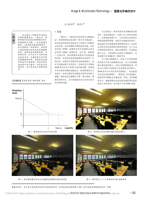
Image & Multimedia Technology ・图像与多媒体技术Electronic Technology & Software Engineering 电子技术与软件工程• 83【关键词】宽动态范围 相机成像 算法相机成像中一种低噪点的宽动态范围算法文/孙凤军1 徐孝天21 引言一般而言,人眼的动态范围是0-10000cd/m 2,然而相机的动态范围一般只有100cd/m 2。
宽动态范围这种技术就是专门用来扩大相机的动态范围,从而来模拟人眼的这种功能。
宽动态范围(WDR )成像技术有时也被称为高动态范围(HDR )成像技术。
近年来,相机被广泛地应用,因此图像的质量也在快速地变得更好,但是宽动态范围成像技术却没有广泛的应用。
这种技术常被用在高端的相机中,而在手机的成像中应用很少。
其原因是大多数的WDR 算法存在计算量大的性能问题。
虽然现在有多种的WDR 成像技术,但每种都有自己的弱点,如何克服这些问题是目前研究的重点课题。
例如如何克服帧率下降、噪点增加、图像处理时间长、芯片性能要求高以及很长的开发周期等问题。
本文将展示一种非常简单的WDR 算法集成在一起的电路设计,克服了以上所涉及的缺点。
在照相机的图片中,人们希望在明亮的区域看到饱和的图像。
因此在过度曝光的部分,通过减少过亮的像素来使图像更真实;但这样会导致本来比较暗的区域变得更暗。
为了让这些黑暗的区域变亮,增益会被使用。
但是增益增大之后,大量的噪点会被带入到图像中,这就是数字化WDR 的一种副作用。
为了减少图像噪点,采用了以周围的像素来联合计算当前像素的办法。
由于这些图像噪点都是临时噪点,由很小的随机数组成,因此可以用取平均值的方法来降低这些噪点。
WDR 技术并不用在所有的图像上,而是被用在高对比度的图像中。
一般来说,对比度越高,则使用的WDR 技术越复杂。
因此一般WDR 算法中,根据图像对比度高低来调控算法的控制因子多而复杂。

基于深度强化学习的自适应滤波算法研究一、引言自适应滤波是指根据信号统计特征,设计出适合当前信号的滤波器。
该技术可用于信号去噪、信号特征提取、信号恢复等领域。
目前,基于深度强化学习的自适应滤波算法受到了广泛关注,并在音频处理、图像处理、控制系统等领域得到了广泛应用。
本文将介绍基于深度强化学习的自适应滤波算法的研究现状与发展方向。
二、自适应滤波的原理及分类自适应滤波是一种根据输入信号的性质调节滤波器响应的方法。
其基本原理是利用输入信号的统计性质、峰值、均值、方差等,调节滤波器的响应特性,使其更加适应当前输入信号的特征。
常用的自适应滤波算法包括最小均方算法(LMS)、归一化LMS算法(NLMS)、递推最小平方算法(RLS)等。
根据滤波器结构,自适应滤波可分为线性自适应滤波与非线性自适应滤波。
线性自适应滤波采用线性滤波器的结构,其输入信号通过滤波器后,输出信号为输入信号与滤波器系数的卷积。
非线性自适应滤波器则不限于线性滤波器的结构,它可以根据需要设计任意结构的滤波器,如模糊滤波器、小波滤波器。
三、深度强化学习及其在自适应滤波中的应用深度强化学习是深度学习与强化学习结合的一种自适应学习方法。
在深度强化学习中,智能体通过与环境的交互,学习如何在特定任务中最大化期望的长期回报。
深度强化学习在语音识别、图像处理、游戏AI、智能机器人等领域得到了广泛应用。
深度强化学习在自适应滤波中的应用主要是基于卷积神经网络(CNN)和循环神经网络(RNN)的结构。
深度强化学习网络利用无监督学习方法,从大量数据中自主学习滤波器的响应特征和滤波器系数。
由于其能够自适应地提取信号的特征,它可以更加准确地去除噪声,从而提高滤波效果。
在实践中,深度强化学习在图像去噪、语音去噪、控制系统等领域得到了广泛应用。
深度强化学习的一个优点是可以取代传统的自适应算法。
传统的自适应滤波器需要在每个时间步骤上计算估计信号,而基于深度强化学习的滤波器可以直接利用输入信号进行学习,省去了估计信号的过程,大大提高了滤波器的运算速度。
第 22卷第 7期2023年 7月Vol.22 No.7Jul.2023软件导刊Software Guide基于视频自适应采样的快速图像检索算法谭文斌1,黄贻望1,2,刘声1(1.铜仁学院大数据学院,贵州铜仁 554300; 2.贵州大学贵州省公共大数据重点实验室,贵州贵阳 550025)摘要:为解决智慧农业监控系统目标图像检索计算量较大、耗时较长的问题,提出一种视频自适应采样算法。
首先,根据视频相邻帧相似度变化情况自适应调整视频帧的采样率以提取视频关键帧,确保提取的关键帧能替代相邻帧参与目标图像检索计算。
然后,将视频关键帧以时间为轴构建视频帧检索算子,代替原视频参与目标图像检索计算,从而减少在视频中检索目标图像时的大量重复计算,达到提升检索效率的目的。
实验表明,自适应采样算法相较于固定频率采样、极小值关键帧算法所构建的视频帧检索算子检出率更高、更稳定。
在确保图像被全部检出的基础上,使用视频帧检索算子替代原视频参与目标图像检索计算的优化幅度较大,时耗减少了60%以上,对提升智慧农业监控系统中目标图像的检索效率具有重要意义。
关键词:自适应采样;图像相似度;目标图像帧;视频帧检索算子DOI:10.11907/rjdk.231260开放科学(资源服务)标识码(OSID):中图分类号:TP391.41 文献标识码:A文章编号:1672-7800(2023)007-0131-07A Fast Image Retrieval Algorithm Based on Video Adaptive SamplingTAN Wenbin1, HUANG Yiwang1,2, LIU Sheng1(1.College of Data Science, Tongren University, Tongren 554300, China;2.Guizhou Provincial Key Laboratory of Public Big Data, Guizhou University, Guiyang 550025, China)Abstract:To solve the problem of high computational complexity and time-consuming target image retrieval in smart agricultural monitoring systems, a video adaptive sampling algorithm is proposed. Firstly, adaptively adjust the sampling rate of video frames based on changes in sim‐ilarity between adjacent frames to extract video keyframes, ensuring that the keyframes extracted by the algorithm can replace adjacent frames in target image retrieval calculations. Then, a video frame retrieval operator is constructed based on the time axis of the video keyframes, re‐placing the original video to participate in the target image retrieval calculation, thereby reducing a large number of repeated calculations when retrieving the target image in the video, and achieving the goal of improving retrieval efficiency. Experiments have shown that the adaptive sam‐pling algorithm has a higher and more stable detection rate than the video frame retrieval operator constructed by fixed frequency sampling and minimum keyframe algorithms. On the basis of ensuring that all images are detected, using video frame retrieval operators to replace the origi‐nal video in the calculation of target image retrieval has a significant optimization range, reducing time consumption by more than 60%, and is of great significance for improving the retrieval efficiency of target images in smart agricultural monitoring systems.Key Words:adaptive sampling; image similarity; target image frame; video frame retrieval operators0 引言近年来随着智慧农业的兴起,种植园逐步实现无人化、自动化和智能化管理。
去噪点的方法Noise reduction is a common challenge in various fields, including photography, audio recording, and signal processing. There are several methods to address this issue, each with its own advantages and disadvantages.去噪是摄影、音频录制和信号处理等各个领域普遍面临的问题。
要解决这个问题,有几种方法可供选择,每种方法都有其优缺点。
One approach to noise reduction is filtering, which involves using algorithms to remove unwanted frequencies or signals from the data. This method is effective in certain scenarios, but it may also result in the loss of important information or introduce unwanted artifacts.一种去噪的方法是滤波,即利用算法从数据中去除不需要的频率或信号。
这种方法在某些情况下很有效,但也可能导致重要信息的丢失或引入不需要的伪影。
Another common method is spectral subtraction, which involves estimating the noise spectrum and subtracting it from the originalsignal. While this approach can be effective in certain situations, it also relies on accurate noise estimation, which can be challenging in real-world scenarios.另一种常见的方法是频谱减法,即估计噪声频谱并从原始信号中减去。
点云模型的噪声分类去噪算法李鹏飞;吴海娥;景军锋;李仁忠【摘要】针对三维点云模型数据在去噪平滑过程中存在的不同尺度噪声和算法计算耗时问题,提出了点云模型的噪声分类去噪算法。
该算法根据噪声点分布特性,将其分为大尺度和小尺度噪声,先利用统计滤波结合半径滤波去除大尺度噪声;然后使用快速双边滤波对小尺度噪声进行平滑,实现点云模型的去噪和平滑。
与传统的双边滤波相比,利用快速双边滤波对点云模型数据进行平滑,有效地提高了计算效率。
实验结果表明,该算法对点云噪声进行快速平滑去除的同时又能有效地保持被扫描物体的几何特征。
%Aiming at the problems that different scale noise exists in denoising and smoothing of 3D point cloud data and time consuming of algorithm, the denoising algorithm for point cloud data based on noise classification is proposed. According to the distribution characteristics, the noise points are divided into large-scale and small-scale noise. Firstly, the large-scale noise is removed by statistical filtering and radius filtering. Then the small-scale noise is smoothed with fast bilateral filtering. Finally, the purpose of denoising and rapid smoothing for 3D point cloud data are achieved. Compared with the traditional bilateral filtering, the computing efficiency is improved using fast bilateral filtering to smooth the point cloud data. The experimental results show that the proposed algorithm can fast denoise and smooth for 3D point cloud data, which can effectively maintain the geometric features of the scanned object.【期刊名称】《计算机工程与应用》【年(卷),期】2016(052)020【总页数】5页(P188-192)【关键词】点云去噪;快速双边滤波;统计滤波;条件滤波;平滑【作者】李鹏飞;吴海娥;景军锋;李仁忠【作者单位】西安工程大学电子信息学院,西安 710048;西安工程大学电子信息学院,西安 710048;西安工程大学电子信息学院,西安 710048;西安工程大学电子信息学院,西安 710048【正文语种】中文【中图分类】TP391.41LI Pengfei,WU Hai’e,JING Junfeng,et al.Computer Engineering and Applications,2016,52(20):188-192.随着点云数据在三维实体造型和虚拟现实中得到越来越广泛的应用,高效率、高精度的数据处理[1]和三维模型重建[2-3]已经成为逆向工程领域的热点研究内容。
FAST BILATERAL FILTERING BY ADAPTING BLOCK SIZE Wei Yu1,Franz Franchetti1,James C.Hoe1,Yao-Jen Chang2,Tsuhan Chen2 1Carnegie Mellon University,2Cornell UniversityABSTRACTDirect implementations of bilateralfiltering show O(r2)com-putational complexity per pixel,where r is thefilter window radius.Several lower complexity methods have been devel-oped.State-of-the-art low complexity algorithm is an O(1) bilateralfiltering,in which computational cost per pixel is nearly constant for large image size.Although the overall computational complexity does not go up with the window radius,it is linearly proportional to the number of quantiza-tion levels of bilateralfiltering computed per pixel in the al-gorithm.In this paper,we show that overall runtime depends on two factors,computing time per pixel per level and aver-age number of levels per pixel.We explain a fundamental trade-off between these two factors,which can be controlled by adjusting block size.We establish a model to estimate run time and search for the optimal block ing this model,we demonstrate an average speedup of1.2–26.0x over the pervious method for typical bilateralfiltering parameters.Index Terms—bilateralfiltering,algorithm complexity, real time1.INTRODUCTIONBilateralfiltering is a non-linearfilter introduced by Tomasi et al.in1998[1].It smoothes out an image by averaging neighborhood pixels like a Gaussianfilter,but preserves sharp edges by decreasing weights of pixels when the intensity dif-ference is large.Bilateralfiltering is useful in many image processing and vision applications such as image denoising [1,2],tone mapping[3],and stereo matching[4].Direct implementation of bilateralfiltering from defini-tion is computationally expensive.There are generally three directions to make an algorithm run faster.First,design lower complexity algorithms without degrading accuracy;second, optimize code extensively for a given algorithm;third,op-timize code on a more powerful hardware platform.In this paper,our focus is along thefirst path.Related work.The computational complexity per pixel for direct implementation is O(r2),where r is thefilter win-dow radius.Recently,several methods have been proposed to reduce the arithmetic complexity of the algorithm.Porikli et al.[5]proposed a constant time bilateralfiltering with respect tofilter size for three types of bilateralfilters.Quantization of image intensity in this method may significantly degrade the quality of thefiltering output.Also,memory footprint re-quirement is large for storing the integral histograms.Yang et al.[6]propose a O(1)bilateralfiltering which extends Du-rand and Dorsey’s piecewise-linear bilateralfiltering method [3].It can achieve O(1)complexity with arbitrary spatial and arbitrary range kernels(assuming the exact or approximated spatialfiltering is O(1)complexity),with much better accu-racy and less memory footprint than[5].In[6],they discretize the image intensities.For each quantization value,they com-pute a linear spatialfiltering,whose output is defined as Prin-ciple Bilateral Filtered Image Component(PBFIC).Thefinal bilateralfiltering output is a linear interpolation between the two closest PBFICs.For typical parameter settings(see sec-tion4),processing time of[6]on a2.67GHz CPU with2GB RAM for image of size600×800is on the order of tens of milliseconds to several seconds.Overview of proposed method.In this paper,we pro-pose an extension of[6],to further reduce the run time based on an important trade-off we found.The overall computing time depends on two factors,the computational cost per pixel per PBFIC,and the average number of PBFICs computed per pixel.O(1)cost per pixel only reflects thefirst factor.We will show there is a fundamental trade-off between these two factors,and changing the block size can control the trade-off.Block size of1×1corresponds to direct implementation, and block size up to the original image size corresponds to the implementation in[6].The optimal block size should be somewhere in between for general cases.We build a model to predict run time given afixed block size,and use this model to search for the best block size.Synopsis.In the following,we briefly review the O(1)bi-lateralfiltering proposed in[6],and explains the fundamental trade-off in Section2.Section3details a model to estimate the computing time.Section4shows experiment results and Section5concludes.2.OBSERV ATION OF A FUNDAMENTALTRADE-OFFFrom the definition of bilateralfiltering,it is a compound of linear spatialfiltering and non-linear rangefiltering.Spatial filtering kernel is usually a simple boxfiltering kernel or a Gaussian kernel,both having O(1)(approximate)algorithms.Proceedings of 2010 IEEE 17th International Conference on Image Processing September 26-29, 2010, Hong KongRangefiltering kernel is usually a Gaussian kernel that assigns lower weight to pixels with large intensity difference.The filter output of a pixel x isI B(x)=y∈N(x)f s(y,x)·f r(I(y),I(x))·I(y)f(y,x)·f(I(y),I(x))f(y,x)·f(I(y),I)256·σ·e)))256·σ,L(b·b)Fig.1.Tradeoff between T a and L a for varying r=2,4,8,16.Here L=K for each block.x-axis showslog2(b w).We only test square blocks of size b w×b w.y-axis shows T a,L a and T a·L a normalized to their maximumvalues.Optimal b w for T a·L a is circled.The above analysis is an approximation of run time.Fig.2further demonstrates the relationship between run time andblock size by measuring the real run time for varying blocksize.We use the same example image.Block size is the sameas in Fig. 1.256σr varies in{1,16}.The code of[6]ispublicly available on website.We simply modify the codesuch that bilateralfiltering is looped on each block.When256σr=1,L=K,the trend of normalized run time withrespect to b w is close to Fig.1.When256σr=16,which isa typical setting for image denoising,increase of L a is muchslower than K for small b w,but T a remains a decreasing func-tion of increasing b w .That is why we observe decreasing run time for small b wvalues.Q R U P D O L ]H G U X Q W L P HFig.2.Measured run time vs.block width,for varying r =2,4,8,16.x-axis shows log 2(b w ).y-axis shows normalized run time to the maximum values.(best view in color)3.PROPOSED MODELIn this section,we build a much more detailed model to es-timate relationship between run time and block size.This model should be accurate enough to enable us to search for optimal or near optimal block size.It should also be simple so that modeling overhead is low.The total run time of bilateral filtering for a block of size b h ×b w includes four parts.•Part 1:time to compute f r (I (y ),I l ))and f r (I (y ),I l )·I (y )in Eq.(2).f r (I (y ),I l )can be pre-computed and stored in a table.For 8-bit intensities,only 256table en-tries are needed.The computing time can be estimated as T 1=C 1(b h +2r )(b w +2r )L .•Part 2:time to compute dividend and divisor in Eq.(2).Both are box spatial filtering,which can be decom-posed into horizontal sum filter followed by a vertical sum filter.For horizontal filter,each row takes 2(b w +r −1)additions/subtractions (after computing summa-tion of neighbors for the first pixel,for consecutive pix-els,summation is computed by adding a new pixel and subtracting an old pixel from the previous summation).Total number of rows is b h +2r .For vertical filter,each column takes 2(b h +r −1)additions/subtractions.To-tal number of columns is b w .So the time is estimated as T 2=C 2((b w +r −1)(b h +2r )+(b h +r −1)b w )L .•Part 3:time to compute division in Eq.(2),estimated as T 3=C 3b h b w L .•Part 4:time to interpolate.The way we implement interpolation is that after computing the l -th level of PBFIC,we check all pixels in the block if I (x )is in [I l −1,I l ).If so,then interpolate as Eq.(3).So roughly speaking,every pixel is checked for L −1times,and only one time its final bilater filtering output is interpo-lated.The time is estimated as T 4=C 4b h b w (L −2)+C 5b h b w .All parameters C 1,C 2,C 3,C 4,and C 5are platform de-pendent,and should be calibrated for each hardware platform.We use the example image in Fig.1and varying b h ,b w to cal-ibrate those parameters.Both log 2b h and log 2b w vary from 2to log 2min(w,h ),and they can be different.For each of the four parts,we use RDTSC()function (Intel time-stamp counter)to measure elapsed time.Fitting C 1,C 2,C 3are sim-ple,e.g.C 3is average of T 3/(b h b w L ).C 4,C 5are estimated using robustfit()in Matlab.We do the experiment on a Dell XPS 720desktop,with Intel Core2Duo E67502.67GHz CPU and 2GB RAM.Esti-mated C 1=28.56,C 2=17.96,C 3=32.45,C 4=32.52,C 5=140.48.Fig.3shows for each of the four parts,the measured run time (T m )and run time predicted from themodel (T p ).Average prediction error (|Tp T −ƉƌĞĚŝĐƚĞĚ ƌƵŶƚŝŵĞ P H D V X U H G U X Q W L P HƉƌĞĚŝĐƚĞĚ ƌƵŶƚŝŵĞ ƉƌĞĚŝĐƚĞĚ ƌƵŶƚŝŵĞ ƉƌĞĚŝĐƚĞĚ ƌƵŶƚŝŵĞFig.3.Measured run time vs.predicted run time from model for part 1–4(Unit for both run time is Giga-cycles).4.EXPERIMENTAL RESULTIn this section,we show how well the model works,and how much speedup can be achieved compared to the method pro-posed in [6].The dataset includes randomly downloaded 50images from website,size ranging from 100×120to 600×800.For bilateral filtering parameters r and σr ,we test r in {2,4,8,16},256σr in {1,2,4,8,16,32},which represent typical range of these parameters.About the model,we are concerned about the following questions.•How much extra cost does this model introduce?•Is the optimal block size searched by this model matches the real optimal one?•If answer to the second question is no,then how much worse is the searched block size from the real one?For the first question,modeling time involves collecting number of quantization levels for a given block size,which needs the information of I min and I max for every block.We limit our search range to all square blocks (b w ×b w ,log 2b w varies from 0to log 2min(w,h )),and all blocks whose height is twice of width (2b w ×b w ,log 2b w varies from 0to log 2min(w,h )−1).For these block sizes,we cansort them in an increasing order,and quantization levels of a certain block size can be easily built from previous block size because current block contains two small previous blocks.The measured modeling time is low.We found for about 97%of all cases,modeling time is less than 10%of the measured run time for the optimal block size.The second and third question relates to modeling accuracy.Fig.4(a)shows pre-dicted run time from modeling (T p )vs.measured run time (T m )for all images and parameter settings we tested.Av-erage prediction error (|Tp T −DEFig.4.(a)Measured run time vs.predicted run time from model;(b)run time of the predicted optimal block size vs.run time of the true optimal block size.(Unit for all run time is Giga-cycles).Next we will show the speedup of using this model over using full image size as block size,which is exactly the O (1)bilateral filtering in [6].Fig.5shows for varying σr ,aver-age speedup over all images vs.r .In each sub figure,the line (with )shows the upper bound of speedup,which is the speedup by using the true optimal block size.The line (with ×)shows the achieved speedup by using the optimal block size predicted by the model.Here we take into ac-count the model overhead.The speedup decreases when r increases.This is consistent with Fig. 1.When r is large,T a becomes the dominating factor in run time,and encour-ages large block size.For large block size,both T a and L a changes slowly with respect to the block size,so the observed speedup is small.The speedup also decreases when σr in-creases,especially for small r .When r is small,L a becomes the dominating factor.However the difference of L a for small and large block sizes becomes smaller when σr gets larger.For example,L a =1for 1×1block,but L a ≈256256σfoV S H H G X SV S H H G X SUORJ UFig.5.Average speedup vs.r over the O (1)bilateral filter-ing in [6]for varying 256σr .The line (with )shows upper bound of speedup by using the true optimal block size,and the line (with ×)shows real speedup of the proposed model.5.CONCLUSIONIn this paper,we show a fundamental trade-off between two factors in the O (1)bilateral filtering method in[6].The two factors are the computing time per pixel per quantization level and the average number of quantization levels per pixel.The trade-off can be controlled by varying block size.We build a timing model to estimate run time for a given block size.Experiments show the model gives reasonably accurate esti-mation of the run time with negligible overhead.More im-portantly,run time of the optimal block size predicted by the model is very close to the run time of the true optimal block size for most cases.Experiments also demonstrates an aver-age speedup of 1.2–26.0x on all images for typical parameter settings.We expect to see even more signi ficant speedup for HDR (high dynamic range)images because intensity ranges of HDR images are usually much larger than 256,which is a typical range of 8-bit digital images.6.REFERENCES[1]Tomasi C.and Manduchi R.,“Bilateral filtering for gray andcolor images,”in ICCV ,1998.[2]A.Buades,B.Coll,and Morel J.M.,“A review of image denois-ing algorithms,with a new one,”in Multiscale Modeling and Simulation ,2005.[3]F.Durand and J.Dorsey,“Fast bilateral filtering for the displayof high-dynamic-range images,”in Proc.of SIGGRAPH ,2002.[4]K.J.Yoon and I.S.Kweon,“Adaptive support-weight approachfor correspondence search,”in IEEE Trans on PAMI ,2006.[5]Fatih Porikli,“Constant time o (1)bilateral filtering,”in Proc.of CVPR ,2008.[6]Qingxiong Yang,Kar-Han Tan,and N.Ahuja,“Real-time o (1)bilateral filtering,”in Proc.of CVPR ,2009.。