国外瞬变电磁法共37页文档
- 格式:ppt
- 大小:3.73 MB
- 文档页数:37
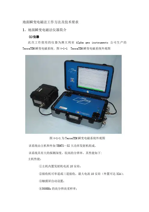
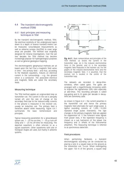
4.4 The transient electromagnetic method (TEM)4.4The transient electromagnetic method (TEM)4.4.1 Basic principles and measuring techniques in TEMBy the transient electromagnetic method, TEM, the electrical resistivity of the underground layers down to a depth of several hundred meters can be measured. Groundbased measurements as well as airborne surveys (SkyTEM) to cover large areas are possible. The method was originally designed for mineral investigations. Over the last two decades the TEM method has become increasingly popular for hydrogeological purposes as well as general geological mapping. The electromagnetic geophysical methods are all based upon the fact that a magnetic field varies in time – the primary field – and thus, according to the Maxwell equations, induces an electrical current in the surroundings – e.g. the ground which is a conductor. The associated electrical and magnetic fields are called the secondary fields.Fig. 4.4.1: Basic nomenclature and principles of the TEM method. (a) Shows the current in the transmitter loop. (b) Is the induced electromotive force in the ground, and (c) is the secondary magnetic field measured in the receiver coil. For the graphs of the induced electromotive force and the secondary magnetic field, it is assumed, that the receiver coil is located in the centre of the transmitter loop.Measuring techniqueThe TEM method applies an ungrounded loop as transmitter coil. The current in the coil is abruptly turned off, and the rate of change of the secondary field due to the induced eddy currents in the ground is measured in the receiver coil, usually an induction coil. The primary field is therefore absent while measuring. Figure 4.4.1 summarizes the basic nomenclature and principles. Typical measuring parameters for a groundbased system are: 1 – 20 ms on-time, 1 – 30 μs turn-off ramp and 1 – 20 ms off-time for measuring. The depicted waveform is often referred to as a square waveform. Other waveforms with sine or triangular shapes are used, but mainly in airborne systems.The datasets are recorded in decay-timewindows, often called gates. The gates are arranged with a logarithmically increasing width to improve the signal/noise (S/N) ratio especially at late-times. This recording principle is called log-gating and 8–10 gates per decade in decaytime are commonly used. As shown in Figure 4.4.1, the current polarities in the transmitter coil and hence the primary magnetic field alternates for each single pulse. A typical sounding consists of 1,000 – 10,000 repeated single pulses (transients). The sign changes in the primary magnetic field are applied for suppression of: 1) the coherent noise signals from power lines, if the repetition frequency is chosen as a sub harmonics of the power line frequency and 2) offsets of the instrumental amplifiers. This measuring technique is referred to as synchronous detection.Field proceduresWhen performing fieldwork, a transient electromagnetic sounding can be conducted by placing a wire in a square loop on the ground as the transmitter coil, Tx-coil. When investigating the upper 150 m of the ground, a square loop65KURT I. SØRENSEN, ANDERS VEST CHRISTIANSEN & ESBEN AUKENwith an area of 40 x 40 m is commonly used. The receiver coil, Rx-coil, with a diameter of approximately 1 m is placed in the centre of the transmitter coil.2The TEM principleThe measurements are carried out by ejecting a current in the Tx-loop. This results in a static primary magnetic field. The current is turned off abruptly and the related change in the primary magnetic field induces an electromotive force in the conducting surroundings. In the ground, this electrical field will result in a current which again will result in a magnetic field, the secondary field. Just after the transmitter is switched off, the secondary magnetic field from the current in the ground will be equivalent to the primary magnetic field (which is no longer there). As time passes by, the resistance in the ground will still weaken the current (converted to heat), and the current density maximum will eventually move outwards and downwards, leaving the current density still weaker. The decaying secondary magnetic field is vertical in the middle of the Tx-loop (at least if the ground consists in plane and parallel layers). Hereby an electromotive force is induced in the Rx-coil. This signal is measured as a function of time. Just after the current in the Tx-loop is turned off, the current in the ground will be close to the surface, and the measured signal reflects primarily the resistivity of the top layers. At later decay-times the current has diffused deeper into the ground, and the measured signal then contains information about the resistivity of the deeper layers. Measuring the current in the Rxcoil will therefore give information about the resistivity as a function of depth. The configurations shown in Figure 4.4.2 have the receiver coil placed in the centre of the Tx-coil and is called a central loop or an in-loop configuration. The receiver coil can be placed outside the Tx-loop which results in an offsetloop configuration.Fig. 4.4.2: Field setup of a TEM system: a) Shows a central loop configuration, b) an offset-loop configuration. Rx denotes the receiver, Tx the transmitter, l the side length of the loop and h the offset between Tx-coil and Rx-coil centres.4.4.2 Data curvesThe decaying secondary magnetic field is referred to as b or the step response. However, because an induction coil is used for measurements of the magnetic field, the actual measurement is that of db/dt, the impulse response (the induced electromotive force is proportional to the time derivative of the magnetic flux passing the coil). The impulse response, db/dt is plotted in Figure 4.4.3 for a variety of halfspace resistivities.Fig. 4.4.3: In a) the impulse responses (db/dt) for a homogeneous halfspace with varying resistivities are presented (black lines). The same curves converted to ρa are shown in b). The grey line is the response of a two-layer earth with 100 Ωm in layer 1 and 10 Ωm in layer 2. Layer 1 is 40 m thick.664.4 The transient electromagnetic method (TEM)Figure 4.4.3 indicates power function dependence at late-times. At late-times, the impulse response can be written as∂b z - Iσ 3 2μ 0 a 2 -5 2 ≈ t ∂t 20π 1 252(4.4.1)As seen db/dt has a decay development -5/2 proportional to t . Observation of the decaying magnetic field in Figure 4.4.3 is not very informative and the same applies for actually measured sounding curves. A plot of apparent resistivity, ρa, is more illustrative. It is derived from the late-time approximation of the impulse responseρa = ( Ia2 μ5 3 )1 / 2 0 3 t -5 3 20 ∂bz ∂t π1(4.4.2)The response curves plotted in Figure 4.4.3a are shown as ρa-converted curves in Figure 4.4.3b. The ρa-converted curves can be used as a data quality tool and as first estimate of the resistivity levels of the underground structure.Fig. 4.4.4: TEM sounding curves stacked with 50 transients (grey) and 5,000 transients (black).4.4.3 Background noiseA geophysical datum always consists of two numbers – the measurement itself and the uncertainty of the measurement. One single transient is affected significantly by the electromagnetic background noise. By repeating and stacking the measurement the background noise is decreased and the signal enhanced. Generally, a TEM sounding may consists of 1,000 to 10,000 single transients. Figure 4.4.4 shows stacks of 50 single transients and a stack of 5,000 single transients. It is obvious that a sounding with 5,000 stacked transients has a much better signal-to-noise ratio, S/N ratio, compared to the stack with 50 transients.The electromagnetic background noise originates from various sources. Most sources, such as lightnings, are very distant. The fields from these sources travel around the globe in the wave guide cavity between the surface of the Earth and the ionosphere. This noise has a random character, and it is more powerful during the day than during the night and stronger during summer compared to winter. Background noise also originates from the power supply and the related man-made electrical installations. There are partly the 50 or 60 Hz signals and its harmonics, which have a deterministic character, partly the transient fields, which are of a random character and related to current changes in the power lines, when various installations are turned on or off. The deterministic part of the background noise from the power supply is removed by synchronous detection techniques, as mentioned before.67KURT I. SØRENSEN, ANDERS VEST CHRISTIANSEN & ESBEN AUKENWith well-designed equipment the noise contribution from the electronics in the instrument itself is negligible compared to the noise contributions described above. It can be shown that using the log-gating technique, random noise contributions are decreasing -1/2 proportional to t . It is evident that the signal level of measurements at early-times in most cases is many times larger than the noise level. This implies that the S/N ratio is high, and the uncertainty of the measurements is low at early-times. At later decay-times the decay signal is proportional to -5/2 t . As the random noise level is proportional to -1/2 t it implies that the transition from a good S/N ratio to a poor S/N ratio happens quite suddenly. There are two ways to obtain datasets of a satisfactory S/N ratio at later decay-times, i.e. information from larger depths: 1) reduce the noise by increasing stack size or 2) increase the transmitted moment. Stacking reduces the noise proportional to N where N is the number of measurements in the stack. The effect of increasing the moment is shown in Figure 4.4.5 with the black dotted line. The line indicates the level of a sounding at the same location with a ten times larger moment and it is clear that the S/N ratio is much higher at later decay-times increased by a factor of ten.Fig. 4.4.5: TEM sounding and noise measurements. The grey curves are noise measurements with the -1/2 t trend plotted with the thick dashed grey line. Error bars are 5%. The earth response is the black curves. The black dotted line indicates the approximate level of a sounding with a 10 times higher transmitter moment.4.4.4 Penetration depthIn relation to TEM soundings it is difficult, as for all other geophysical methods, to speak quantitatively and unambiguously about the penetration depth. In the following we will state some rules of thumb. The depth down to which the current system has diffused is called the diffusion depth. This depth, zd, is defined byThis is an exact equation for plane fields only. For circular or quadratic loop sources the diffusion depth is about 1.8 times smaller than estimated by Equation 4.4.3. As seen in the Figure 4.4.3, the signal decreases -5/2 in a homogenous halfspace by t , and when the signal passes the level of the background noise, we can no longer use the measurements. Thus, the level of the background noise sets the limits for how late we can use our measurements. By using the expression given for dbz/dt for latetimes we find a relationship between the noise signal, Vnoise, and the latest decay-time at which we can make measurements:zd =2t ≈ .26 × ρt [m] , 1 μσρ [Ωm], t [μs](4.4.3)684.4 The transient electromagnetic method (TEM)tL = μ (M )2 / 5 20 Vnoiseσ ( )3 / 5 π(4.4.4)When tL is equivalent with the diffusion time tdzd = ( 2 1 / 10 ) 25 π 3 ( M 1/ 5 M 1/ 5 ) = 0.551 ( ) σVnoise σVnoisedataset within the estimated uncertainties are called equivalent models. Sometimes equivalences can be very pronounced in the sense that very different models give rise to almost identical responses. Equivalence appears in relation to thin good conductors embedded in resistive surrounding and vice versa. In these cases the resolution of the thin layers may be poor resolved.(4.4.5)From these expressions it is seen that the maximal diffusion depth, which is a measure for the penetration depth, is proportional to the fifth root of the ratio between the moment of the current loop and the product of the conductivity and the noise level. The only way to increase the penetration depth is to increase the moment of the transmitter or decrease the effective noise level, being the noise level after stacking and gating. The background noise is a relatively unchangeable size, but the way in which we gather and process our datasets, by stacking many measurements, reduces the effective noise. To double the penetration depth, the effective noise has to be reduced – or – the moment of the transmitter has to be increased by a factor 32.4.4.6 Coupling to man-made installationsDistortion of datasets due to coupling to manmade electrical installations is not noise in the same sense as the random electromagnetic background noise described in the noise section. Coupling noise is a distortion and relates to induced currents in all man-made electrical conductors. The distortion has a deterministic character, arising at the same delay time for all decays and will therefore be summed in the stacking process. Coupling distortion in datasets cannot be accurately removed to provide a reliable interpretation; therefore soundings located close to man-made installations such as pipelines, cables, power lines, rails, auto guards and metal fences cannot be interpreted, and the dataset should be culled. The safe distance, defined as the minimum distance where undistorted datasets can be measured, is counted as the distance between any point on the transmitter-receiver setup and the man-made conductor. The safe distance to any man-made conductor is at least 100 m over an earth with an overall resistivity of 40 – 60 Ωm. The safe distance increases with the resistivity.4.4.5 Resolution and equivalenceThe induced eddy currents are predominantly flowing in the good conducting formations. Therefore the resistivity and the layer boundaries of good conductors are very often well resolved. The eddy currents decay fast in high resistive layers and only weak measurable signals are produced. Hence in the presence of good conductors these signals often are neglectable and the resistivity level of high resistive formations is poorly resolved. In contrary, the layer boundaries may be resolved as these will coincidence with the boundaries of good conductors. The “geometry” of the high resistive formations may therefore be resolved. As mentioned before a geophysical measurement is described by its value and the uncertainty estimate on this value. Models that produce responses which compare to the measured4.4.7 Modelling and interpretation Data acquisitionAs mentioned in the introduction, a main issue in applying the TEM method for hydrogeological studies is the demand for accurate and undisturbed datasets with high spatial density. Insufficient data quality makes it impossible to obtain a reliable geophysical model for use in a hydrogeological context.69KURT I. SØRENSEN, ANDERS VEST CHRISTIANSEN & ESBEN AUKENAn important element of the data quality is the precise knowledge of the parameters of the applied instrument. To obtain datasets of sufficient quality, the following instrumental parameters must be known and modelled in the data modelling algorithm:■■The transmitted waveform characteristics, including the exact appearance of the current turn-off and turn-on ramps and the timing between the transmitter and the receiver actions. Timing parameters must be known to an accuracy of 100 – 200 nanoseconds, because of their severe impact on early-time data. The receiver transfer function, which is modelled by one or more low-pass filters, often has a strong influence on early-time data. Low-pass filters are implemented in the receiver system to stabilize the amplifiers and to suppress the noise from long-wave radio transmitters. The geometry of the transmitter-receiver configuration must be accurate, especially for the offset-loop configuration. Central-loop datasets are relatively insensitive to deviations in geometry as long as the transmitter area is unchanged.■Measuring in the central-loop configuration with a small transmitter coil and high output current may saturate the receiver amplifiers due to high voltages arising from the turn-off of the primary field. After saturation, amplifiers will produce distorted signals for several milliseconds. Furthermore, currents of the order of nanoamperes will leak in the transmitter coil after the current is turned off, adding to the earth's response and thereby to the distortion of the datasets. Both effects become negligible because of geometry when using either a small output current with a large transmitter loop or a large offset between the transmitter and the receiver coils. Thus high-output current datasets using a small transmitter coil must be measured in the offset-loop configuration, while low current datasets can be measured in the central-loop configuration. The induced polarization (IP) effect is present in datasets measured in some sedimentary environments. The IP effect is most pronounced in datasets from the central-loop configuration, but moves to later decay-times when increasing the transmitter coil size. In offset configurations the IP effect is less pronounced and moves to later decay-times as the offset between the transmitter and the receiver coil is increased. At early times, measurements using the offset configuration are extremely sensitive to small variations in the resistivity in the near surface. Extensive 3D modelling of such variations shows a pronounced influence on the measured datasets as the current system passes beneath the receiver coil. In many cases these datasets are not interpretable with a 1D model, even if the section is predominantly 1D. At later times, after the current system has passed, the distorting influence has decayed. Datasets from the central-loop configuration are much less affected by near-surface resistivity variations. Datasets from the offset configuration are sensitive to small deviations in the array geometry. As an example assuming a 60 Ωm half-space model, a 30% error in the decay signal is apparent near the sign change if the receiver coil is located 71 m instead of 70 m■■Measuring datasets with a high spatial density serves two purposes: 1) the resolution of geological structures is improved and 2) distorted datasets caused by instrument malfunction and transmitter-induced coupling to man-made conductors can be revealed and eliminated. The latter is by far the most important.■Configurations, advantages and drawbacksGround-based TEM systems using a high transmitter moment normally utilize a transmitter loop of 40 – 100 m. The advantages of a large loop are that measurements can be carried out at the centre of the loop, and that the magnetic moment is large. The drawbacks are the low field efficiency and the higher possibility of coupling with man-made installations. A small transmitter coil with a high current is very field efficient, but four issues must be tackled in the configuration design:■704.4 The transient electromagnetic method (TEM)from the transmitter. In a routine field situation, it is next to impossible to work with such accuracy. After the sign change, datasets from the offset configuration is essentially equivalent to that of a central-loop configuration. A compromise is to use a high-power system with small transmitter loop, where early-time data are measured in the central loop configuration with a small current of 1 – 3 A. Late-time data are, in turn, measured in the offset configuration with maximum output current. In this way the four issues are addressed, and the field productivity can still be kept high.number of key issues need to be addressed to achieve this high data quality. The issues are mainly related to calibration, altitude and the flight speed.CalibrationIn the context of requiring high data quality, the calibration of the transmitter/receiver system plays a central role. When airborne systems operate in the frequency domain, the strong primary field has to be compensated in order to be able to measure the Earth response. Because of drift in the system the compensation changes in time, and its value has to be determined successively during the survey by high-altitude measurements. Furthermore, it is necessary to perform measurements along tie lines perpendicular to the flight lines and by postprocessing to provide concordance between adjacent lines. This process is called levelling, and because of this a frequency domain system is said to be relatively calibrated. When airborne systems are operating in the time domain, it is possible to reduce the interaction between the transmitter and the receiver system to a level, at which the distortion of the measured off-time signals is negligible. In this case, a calibration of the instrumentation can be performed in the laboratory and/or at a testsite before carrying out the surveys. Neither high altitude measurements nor performing tie lines for levelling are then necessary during the survey. Such a system is said to be absolute calibrated. The SkyTEM system has these capacities. The relatively calibrated systems will have a lower S/N ratio and lower data accuracy because of the drift and the levelling of datasets compared to that of absolutely calibrated systems.The 1D modelTo this day it is not possible to invert TEM datasets in more than one dimension on a routine basis. 3D inversion codes have been developed lately, but they are still computationally very demanding, and require densely measured datasets in at least two dimensions. Therefore, it is inevitable that geological noise, i.e. insufficient model presentation of the actual structure, is present when describing a 3D structure by a 1D model. The distribution of 2D and 3D structures decides the amount of geological noise.4.4.8 Airborne TEMBelow we will present an overview of the requirements to airborne EM systems, especially TEM, and discuss the specific topics where the airborne and the ground based techniques differ. We will focus on the relatively new helicopter system, SkyTEM, as it provides the sufficient accuracy necessary for groundwater investigations. Hence the following comment on the main issues for airborne TEM is related to the application of the SkyTEM method.AltitudeFor all EM airborne systems the Earth response decreases with increasing altitude. The random noise contribution from natural and man-made sources show no significant decrease within the operating altitude range compared toSpecial considerations for airborne electromagnetic measurementsIn groundwater exploration, high quality data are required as the decisive data changes can be as low as 10 – 15 %. When operating airborne a71KURT I. SØRENSEN, ANDERS VEST CHRISTIANSEN & ESBEN AUKENground based measurements. Therefore, a higher operating altitude implies a lower S/N ratio at late-times, where the noise becomes predominant, and results in a poorer resolution of the deeper part of the Earth. The resolution of the near-surface layers decreases with increasing altitude because the induced eddy current system at early-times becomes larger and more spatial averaged. In general, increasing altitude means a lower resolution of upper layers. Another implication of the decaying Earth response with altitudes is increased distortions of the Earth response due to coupling to man-made installations. As mentioned before, a safety distance to installations of at least 100 m, depending on the subsurface structures, has to be maintained in order to avoid distorted datasets. Application of airborne electromagnetic measurements introduces larger safety distances to installations compared to ground based equipment, because Earth responses decreases with increasing altitude, whereas coupling responses in the operation altitudes maintain their signal level. The larger the operating altitude is the larger are the safety distances.The lateral movement while achieving the required stack size increases with velocity which implies a decrease in the lateral resolution. Hence, a higher vertical resolution inevitably means a decreased lateral resolution if the fight speed is unchanged. On the contrary, the same lateral resolution at a higher velocity results in a decrease of the S/N ratio and hence the vertical resolution.Data quality and post-processingAirborne electromagnetic surveys are very cost effective. As the data acquisition is extremely fast, and large amounts of datasets are collected over a short period of time, the data quality control has to be automatic. As discussed before, the application of an absolutely calibrated TEM system, as the SkyTEM system, implies that no high-altitude measurements have to be carried out during the survey and subsequently used for compensating the datasets for the effects from transmitterreceiver interactions. Nor is it necessary to perform levelling of the datasets. In order to maintain the high data quality demanded for groundwater surveys, the geometrical setup of the equipment has to be well determined at all times, as well as the transmitted current waveform. The geometrical setup is determined by the altitude and the inclination of the transmitter and receiver coils. Furthermore, it is essential that the calibration and the functionality of the instruments are well documented, and that all setup parameters are saved for the subsequent interpretation. The post-processing of the measured datasets relates to two tasks. The first task is to process the altitude, inclination and position data in order to remove outliers and to provide continuity. Especially the altitude data need processing as they are, in many cases, affected by the vegetation on the surface. If the altimeter reflections from vegetation are not identified and corrected, errors will be introduced in the interpreted models. Figure 4.4.6 shows a section of altimeter data from the SkyTEM system. The dots are reflections as picked up by one of the laser altimeters mounted on the transmitterFlight speedAn important tool for increasing the S/N ratio in electromagnetic measurements is to perform stacking of the measurements. In TEM measurements the background noise is reduced by stacking the transients. To achieve a required S/N ratio, a certain number of transients are necessary in the stack. When the system is moving while measuring, a trade-off exists between the lateral and the vertical resolution of the Earth parameters because a flight velocity related time interval is needed to collect the transients for the required stack size. The vertical resolution is related to the S/N ratio determined by the stack size. A certain stack size corresponds to a defined acquisition time interval.724.4 The transient electromagnetic method (TEM)frame. The solid line is the processed altimeter data. The effects of the erroneous reflections obtained over the forest are removed in the processed altitude curve. Data from the processed altimeter data are used in the interpretation of the datasets.Fig. 4.4.6: Processing of altitude data. Dots are the actual reflections picked up by a laser altimeter. The solid line is the processed height data. Over the forest a large number of reflections come from the tree-tops.The measured inclination of the frame is used both to correct the altitudes and the datasets. Altitudes are measured assuming that the laser beam is normal to the ground surface. When the laser tilts, the normal altitude has to be calculated. The data compensation arises because it is assumed that the transmitter and the receiver are z-directed. This is not true when the frame is tilted. The second task is related to the distorting of the datasets by the coupling responses from manmade installations. This is a very time consuming process when operating in culturally developed countryside and involves a significant part of the post-processing time. However, the removal of coupling-distorted datasets is crucial for the quality of the interpreted datasets. Figure 4.4.7 is an example from a SkyTEM survey where the survey line crosses two couplings associated with roads. The data marked with grey in Figure 4.4.7a are coupled, and like the sounding curve in Figure 4.4.7c they can not be used for interpretation. The uncoupled data in Figure 4.4.7b have a smooth appearance in the whole time range until they reach the noise level for the last couple of gates.Fig. 4.4.7: Coupled datasets. Panel a) is a plot of selected time gates along a profile from a SkyTEM survey. Data are normalized with the transmitter moment. Datasets marked with grey are identified as coupled whereas black data are uncoupled. The coupled datasets are associated with the crossing of two roads. Plot b) shows a coupled dataset, and for comparison an uncoupled dataset is shown in c). Profile and position of selected soundings are shown on the inserted map in d). The coupled sounding is marked with a circle, the uncoupled sounding with a square. The thick solid line marks the profile section shown in a).4.4.9 The SkyTEM systemThe SkyTEM system has been developed for groundwater investigations by the HGG group at the University of Aarhus, Denmark. During the last 4 years, the system has been intensively used for groundwater surveys. A key issue for the system development was that the measured datasets present the same quality as those from the groundbased TEM systems. The transmitter and receiver coils, power supplies, laser altimeters, inclinometers, global positioning system (GPS), electronics, and data logger are carried as a sling load on the cargo hook of the helicopter. SkyTEM in operation is pictured in Figure 4.4.8.73。

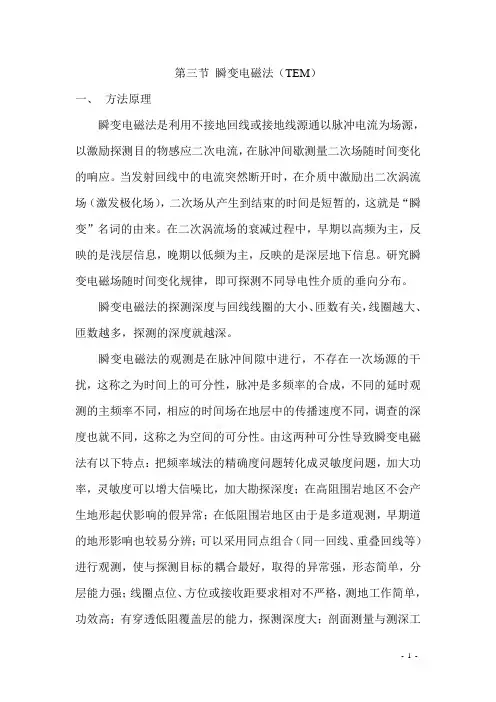
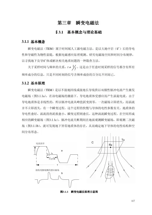
第三节瞬变电磁法(TEM)一、方法原理瞬变电磁法是利用不接地回线或接地线源通以脉冲电流为场源,以激励探测目的物感应二次电流,在脉冲间歇测量二次场随时间变化的响应。
当发射回线中的电流突然断开时,在介质中激励出二次涡流场(激发极化场),二次场从产生到结束的时间是短暂的,这就是“瞬变”名词的由来。
在二次涡流场的衰减过程中,早期以高频为主,反映的是浅层信息,晚期以低频为主,反映的是深层地下信息。
研究瞬变电磁场随时间变化规律,即可探测不同导电性介质的垂向分布。
瞬变电磁法的探测深度与回线线圈的大小、匝数有关,线圈越大、匝数越多,探测的深度就越深。
瞬变电磁法的观测是在脉冲间隙中进行,不存在一次场源的干扰,这称之为时间上的可分性,脉冲是多频率的合成,不同的延时观测的主频率不同,相应的时间场在地层中的传播速度不同,调查的深度也就不同,这称之为空间的可分性。
由这两种可分性导致瞬变电磁法有以下特点:把频率域法的精确度问题转化成灵敏度问题,加大功率,灵敏度可以增大信噪比,加大勘探深度;在高阻围岩地区不会产生地形起伏影响的假异常;在低阻围岩地区由于是多道观测,早期道的地形影响也较易分辨;可以采用同点组合(同一回线、重叠回线等)进行观测,使与探测目标的耦合最好,取得的异常强,形态简单,分层能力强;线圈点位、方位或接收距要求相对不严格,测地工作简单,功效高;有穿透低阻覆盖层的能力,探测深度大;剖面测量与测深工作同时完成,提供了更多有用信息,减少了多解性。
二、地球物理前提由于瞬变电磁法是观测断电后由一次脉冲激励出的二次涡流场随时间的变化规律,二次涡流场随时间的衰减快慢和强弱与被探测介质(道碴、混凝土、岩石等)及介质状态(含水与干燥、完整与破裂)有关,TEM法衰减曲线的变化过程反映了检测点由高频到低频、由浅层到深层的地质信息变化过程。
检测的参数是各层规一化的电阻率,对实测的衰减曲线进行反演拟合,绘制地下电性分层及分层的电阻率柱状图,进而以反演拟合曲线为基础,绘制成曲线簇断面图、等值线断面图及电性分级断面图。
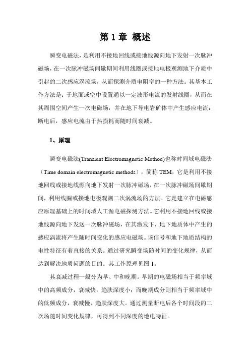
第1章概述瞬变电磁法,是利用不接地回线或接地线源向地下发射一次脉冲磁场,在一次脉冲磁场间歇期间利用线圈或接地电极观测地下介质中引起的二次感应涡流场,从而探测介质电阻率的一种方法。
其基本工作方法是:于地面或空中设置通以一定波形电流的发射线圈,从而在其周围空间产生一次电磁场,并在地下导电岩矿体中产生感应电流:断电后,感应电流由于热损耗而随时间衰减。
1、原理瞬变电磁法(Transient Electromagnetic Method)也称时间域电磁法(Time domain electromagnetic methods),简称TEM,它是利用不接地回线或接地线源向地下发射一次脉冲磁场,在一次脉冲磁场间歇期间,利用线圈或接地电极观测二次涡流场的方法。
它是建立在电磁感应原理基础上的时间域人工源电磁探测方法。
它利用不接地回线或接地线源向地下发送一次脉冲磁场,在其激发下,地下地质体中产生的感应涡流将产生随时间变化的感应电磁场。
该信号和地下地质结构的电性特征有着直接的关系。
通过研究瞬变场随时间的变化规律,从而达到解决地质问题的目的。
其工作原理见图1。
其衰减过程一般分为早、中和晚期。
早期的电磁场相当于频率域中的高频成分,衰减快,趋肤深度小;而晚期成分则相当于频率域中的低频成分,衰减慢,趋肤深度大。
通过测量断电后各个时间段的二次场随时间变化规律,可得到不同深度的地电特征。
瞬变电磁法是在没有一次场背景情况下观测研究二次场,简化了对探测目标产生异常的研究。
该方法以其装置轻便、受旁侧影响小、高工效、低成本等特点已被广泛用于金属矿和煤田地质勘探、工程物探、地下水与地热勘探、采空区与岩溶发育带探测及环境灾害地质调查研究等诸多领域。
由于方法本身的属性,不宜在高压超高压输变电线路、铁路等强干扰源附近采集资料,这也为相关规范、技术规程所规定。
2、优点瞬变电磁法探测具有如下优点⑴由于施工效率高,纯二次场观测以及对低阻体敏感,使得它在当前的煤田水文地质勘探中成为首选方法;⑵瞬变电磁法在高阻围岩中寻找低阻地质体是最灵敏的方法,且无地形影响;⑶采用同点组合观测,与探测目标有最佳耦合,异常响应强,形态简单,分辨能力强;⑷剖面测量和测深工作同时完成,提供更多有用信息。

瞬变电磁法1、概述顺便电磁法(TEM)属于时间域电磁法,它是的原理是根据地壳中岩石或者矿体的导电性及介电性等电学性质的差异,以不接地的回线或者是连接地线通上脉冲电流为场源,地下发射一次脉冲磁场,在一次脉冲磁场间歇期间利用线圈或接地电极观测地下介质中引起的二次感应涡流场,从而探测介质电阻率的一种方法。
其基本工作方法是:于地面或空中设置通以一定波形电流的发射线圈,从而在其周围空间产生一次电磁场,并在地下导电岩矿体中产生感应电流:断电后,感应电流由于热损耗而随时间衰减,有一个瞬变的过程。
可以通过判断和分析二次的时空变化特征,来判断地下地质体的电性特征,找出其位置,产状和埋深等特征。
具有可以同时的具有时间和空间的可分性、探测深度达、分辨率高、信息丰富等优点。
近几十年来,我国科学技术快速进步,经济迅猛发展,各项基础建设稳步展开,对于各种矿产资源、能源、地下水资源等的需求快速增加。
同时,各项建设中遇到了许多工程问题,如公路建设中的地下空洞、煤田开采中的陷落柱、隧道开挖中的突水问题等等。
这些因素在一定程度上制约着我国经济的发展,而顺便电磁法的出现,利用其测量方面的优势,已经发展成为探测油气、金属和非金属矿产的一种重要方法,并且在深部地质构造研究,工程勘察、油气、矿产、水、地热勘探等领域得到了广泛的应用。
可以很好地保证资源供给,减少经济损失,加快建设进度。
2、研究现状2.1、研究历史对勘测工程工作的种种困难,把瞬变电磁法应用到地质勘探中的想法在上世纪30年代就有人提出来。
最初的时域电磁法是利用到了L.W.Blan在1993年获得专利,用电磁脉冲激发提供电偶极形成电场。
随后在前苏联有人提出了瞬变电磁测深法。
在50年代,前苏联、加拿大、美国等国已经开始就瞬变电磁法的理论与应用技术进行了深入的研究,同时期由J.R.Wait 提出了使用瞬变电磁场法寻找导电矿体的理念。
前苏联也基本已经建立了瞬变电磁法与野外施工的技术方法,更在70、80年代开展了大量的测量工作,特别是在二维和三维测量的方面就有了很大的进步,这使的瞬变电磁法在地质勘探上运用有了很大的发展。