A Comparison of FPGA and GPU for Real-Time Phase-Based Optical Flow,Stereo, and Local Image Features
- 格式:pdf
- 大小:2.15 MB
- 文档页数:14

代号分类号学号密级10701TP37公开1102121253题(中、英文)目基于GPU/多核CPU平台下并行计算的实时超分辨和立体视图生成Real-time Super-resolution and Stereoscopic View Genera-tion with GPU/Multicore CPU Based Parallel Computing 作者姓名孙增增指导教师姓名、职务郑喆坤教授学科门类工学提交论文日期二〇一四年三月学科、专业模式识别与智能系统西安电子科技大学学位论文独创性(或创新性)声明秉承学校严谨的学风和优良的科学道德,本人声明所呈交的论文是我个人在导师指导下进行的研究工作及取得的研究成果。
尽我所知,除了文中特别加以标注和致谢中所罗列的内容以外,论文中不包含其他人已经发表或撰写过的研究成果;也不包含为获得西安电子科技大学或其它教育机构的学位或证书而使用过的材料。
与我一同工作的同志对本研究所做的任何贡献均已在论文中做了明确的说明并表示了谢意。
申请学位论文与资料若有不实之处,本人承担一切的法律责任。
本人签名:日期:西安电子科技大学关于论文使用授权的说明本人完全了解西安电子科技大学有关保留和使用学位论文的规定,即:研究生在校攻读学位期间论文工作的知识产权单位属西安电子科技大学。
学校有权保留送交论文的复印件,允许查阅和借阅论文;学校可以公布论文的全部或部分内容,可以允许采用影印、缩印或其它复制手段保存论文。
同时本人保证,毕业后结合学位论文研究课题再撰写的文章一律署名单位为西安电子科技大学。
(保密的论文在解密后遵守此规定)本人授权西安电子科技大学图书馆保存学位论文,本学位论文属于(保密级别),在年解密后适用本授权书,并同意将论文在互联网上发布。
本人签名:日期:导师签名:日期:摘要近些年来,许多因素导致了计算产业转向了并行化发展的方向。
在这过程中,受市场对实时、高清晰3维图形绘制的需求驱使,可编程的图形处理单元(GPU)逐渐发展进化成为了具有强大计算能力、非常高内存带宽的高度并行、多线程的众核处理器。

第46卷 第3期2024年3月系统工程与电子技术SystemsEngineeringandElectronicsVol.46 No.3March2024文章编号:1001 506X(2024)03 0795 10 网址:www.sys ele.com收稿日期:20230313;修回日期:20230616;网络优先出版日期:20230818。
网络优先出版地址:http:∥link.cnki.net/urlid/11.2422.TN.20230818.1441.002基金项目:国家自然科学基金(U1934222,62027809,U2268206);北京交通大学人才基金(2022XKRC003)资助课题 通讯作者.引用格式:王子涵,巴晓辉,姜维,等.基于GPU的北斗B1宽带复合信号实时发生器设计[J].系统工程与电子技术,2024,46(3):795 804.犚犲犳犲狉犲狀犮犲犳狅狉犿犪狋:WANGZH,BAXH,JIANGW,etal.Real timedesignofwidebandcompositesignalgeneratorforBeidouB1basedonGPU[J].SystemsEngineeringandElectronics,2024,46(3):795 804.基于犌犘犝的北斗犅1宽带复合信号实时发生器设计王子涵1,巴晓辉1,2,3, ,姜 维1,2,3,蔡伯根2,3,4,王 剑1,2,3,文 韬1,2,3(1.北京交通大学电子信息工程学院,北京100044;2.北京交通大学轨道交通控制与安全国家重点实验室,北京100044;3.北京市电磁兼容与卫星导航工程技术研究中心,北京100044;4.北京交通大学计算机与信息技术学院,北京100044) 摘 要:为了实现北斗B1C+B1I信号的联合生成,提出一种基于软件无线电和图形处理器(graphicsprocessingunit,GPU)加速的北斗B1宽带复合信号的实时生成方法,该方法针对单边带复数二进制偏移载波(single sidebandcomplexbinaryoffsetcarrier,SCBOC)调制方式的信号体制进行设计,系统根据用户配置的接收机运动轨迹和星历文件,生成中频信号并通过射频端发射。

行业研究东兴证券股份有限公司证券研究报告FPGA提供了什么价值?——“FPGA五问五答”系列报告一投资摘要:FPGA(可编程逻辑门阵列)又称“万能芯片”,美国禁运后,作为最“卡脖子”的芯片之一而家喻户晓。
虽然全球市场规模只有80亿美元,FPGA这个不大不小的市场却撑起了龙头赛灵思近500亿美元的市值(英特尔平均市值在2000亿美元上下,所在市场规模是FPGA的10倍)。
目前,全球90%的市场份额由美国FPGA厂商垄断,国产替代必要性不言而明。
美国禁运后,国产FPGA厂商迎来发展的历史性机遇。
FPGA究竟有什么价值?什么在驱动它的未来的成长?龙头为什么能有这么高的市场份额?护城河在哪里?本土厂商又要如何培育自己的竞争优势?针对这些问题,我们复盘了FPGA三大厂商:赛灵思、Altera和Lattice的发展历程,总结出了核心规律,并在FPGA五问五答系列报告中逐一为投资者解答。
作为我们FPGA五问五答第一篇,在这篇报告中,我们首先回答一个最关键的问题——FPGA提供了什么价值?为了回答这个问题,我们仔细研究了FPGA和其他处理器的架构演变和历史,回答如下:FPGA无可比拟的灵活性,以及确定性的低时延优势,是FPGA难以被替代的原因,也是FPGA为客户提供的独一无二的价值。
FPGA是什么?在半导体产业链中的位置?芯片分为模拟芯片和数字芯片,数字芯片负责处理数字信号,分为处理器、逻辑、存储三大类。
FPGA是可编程的逻辑芯片,和其它逻辑芯片的不同之处在于,用户可以随时定义其硬件功能。
虽然FPGA市场仅占逻辑芯片的5%,市场规模仅有微处理器的大约十分之一,但在许多领域是不可或缺的。
FPGA为什么在历史上脱颖而出?PLD诞生的动因来自于ASIC和ASSP的不足,通过可编程来满足降低芯片设计风险的需求。
FPGA并不是第一个被创造出来的可编程逻辑器件,但由于FPGA的架构弥补了PLD和ASIC/ASSP的缺环,能够满足下游不断增长的容量和速度的需求,在发明后的10年开始飞速替代SPLD和CPLD,成为独占鳌头的可编程逻辑器件。

2024年普通高等学校招生全国统一考试(新课标Ⅰ卷)英语学科姓名________________准考证号________________全卷共12页,满分150分,考试时间120分钟。
考生注意:1.答题前,请务必将自己的姓名、准考证号用黑色字迹的签字笔或钢笔分别填写在试题卷和答题纸规定的位置上。
2.答题时,请按照答题纸上“注意事项”的要求,在答题纸相应的位置上规范作答,在本试题卷上的作答一律无效。
第一部分听力(共两节,满分30分)做题时,先将答案标在试卷上。
录音内容结束后,你将有两分钟的时间将试卷上的答案转涂到答题纸上。
第一节(共5小题;每小题1.5分,满分7.5分)听下面5段对话。
每段对话后有一个小题,从题中所给的A、B、C三个选项中选出最佳选项。
听完每段对话后,你都有10秒钟的时间来回答有关小题和阅读下一小题。
每段对话仅读一遍。
例:How much is the shirt?A.£19.15.B.£9.18.C.£9.15.答案是C。
1.【此处可播放相关音频,请去附件查看】What is Kate doing?A.Boarding a flight.B.Arranging a trip.C.Seeing a friend off.2.【此处可播放相关音频,请去附件查看】What are the speakers talking about?A.A pop star.B.An old song.C.A radio program.3.【此处可播放相关音频,请去附件查看】What will the speakers do today?A.Go to an art show.B.Meet the man's aunt.C.Eat out with Mark.4.【此处可播放相关音频,请去附件查看】What does the man want to do?A.Cancel an order.B.Ask for a receipt.C.Reschedule a delivery.5.【此处可播放相关音频,请去附件查看】When will the next train to Bedford leave?A.At9:45.B.At10:15.C.At11:00.第二节(共15小题;每小题1.5分,满分22.5分)听下面5段对话或独白。

gpu 推理英语GPU Inference in EnglishGPU inference refers to the use of a graphics processing unit (GPU) for performing推理 tasks in deep learning and artificial intelligence applications. GPUs are specialized processors designed to handle parallel computations, making them well-suited for accelerating inference workloads.During the inference phase, a trained neural network model is used to make predictions or inferences on new data. Instead of processing the data on a central processing unit (CPU), GPUs can be utilized to expedite the inference process. By offloading the computations to the GPU, significant performance gains can be achieved, enabling real-time or near-real-time inference.GPU inference offers several benefits, including high throughput and low latency. GPUs possess a large number of cores and can simultaneously process multiple data elements in parallel, resulting in faster inference speeds. This is particularly beneficial for applications such as image recognition, natural language processing, and video analysis, where large amounts of data need to be processed in a timely manner.To perform GPU inference, deep learning frameworks and libraries often provide GPU-optimized versions or extensions. These frameworks leverage the parallel computing capabilities of GPUs to accelerate the execution of neural network models. By using CUDA (Compute Unified Device Architecture) or other GPU programming interfaces, developers can explicitly program the GPU to optimize the inference workflow.GPU inference is becoming increasingly prevalent in various industries, including healthcare, finance, autonomous vehicles, and entertainment. It allows for the deployment of complex AI models on edge devices or in the cloud, enabling real-time decision-making and enhanced user experiences.In summary, GPU inference leverages the parallel processing power of GPUs toaccelerate the inference process in deep learning and artificial intelligence applications, offering improved performance and efficiency.。

0引言深度卷积神经网络(Convolutional Neural Network ,CNN)已经成为了当前计算机视觉系统中最有前景的图像分析方法之一。
近年来,随着Binary-Net 、Dorefa-Net 、ABC-Net 等[1-3]低精度量化神经网络的深入研究,越来越多的研究集中于在FPGA 硬件中构建定制的加速器结构,实现CNN 的加速[4]。
基于FPGA 的低精度量化神经网络实现主要可分为两类:流架构[5-6]和层架构[7-8]。
其中,由于流架构实现了流水线化,每个阶段都可以独立处理输入且可以针对CNN 逐层设计并优化相应层的加速运算单元,因此拥有更高的吞吐率和更低的延迟以及内存带宽,但其逻辑资源等消耗也相当可观。
因此,现有的基于流架构实现的二值神经网络加速器研究大多是针对32×32尺度MNIST 数据集等小尺度的图像输入。
而实际应用中更多使用如448×448尺度的YOLO 、224×224尺度的VGG 等作为骨干网络,一方面,大尺度输入的网络结构参数量往往较大(以VGG 为例,其参数量大约500MB),高端FPGA 的片上内存容量也仅32.1Mb 左右,这对FPGA 实现CNN 加速将是资源瓶颈。
即使采用低精度量化策略,FPGA 有限的片上内存资源仍捉襟见肘。
另一方面,虽然各层运算单元可以得到特定优化,然而由于网络拓扑结构限制,往往各层网络很难实现计算周期的匹配,从而造成推断性能难以进一步提高。
针对基于流架构的二值卷积神经网络加速器设计存在的资源与性能的瓶颈,本文以224×224尺度的VGG-11网络加速器设计为例,重点研究了大尺度的二值卷积神经网络硬件加速器设计、优化及验证,主要工作如下:(1)针对大尺度流架构的二值VGG 卷积神经网络加速器设计存在的资源与性能瓶颈,提出了网络模型优化二值VGG 卷积神经网络加速器优化设计∗张旭欣,张嘉,李新增,金婕(上海工程技术大学电子电气工程学院,上海201600)摘要:基于FPGA 的二值卷积神经网络加速器研究大多是针对小尺度的图像输入,而实际应用主要以YOLO 、VGG 等大尺度的卷积神经网络作为骨干网络。

FPGA,GPU和CPU在高性能计算领域的应用及展望课程:系统及可编程芯片设计专业:微电子学与固体电子学姓名:学号:任课老师:FPGA,GPU和CPU在高性能计算领域的应用及展望目前FPGA对于浮点数的运算速度已经达到1TFLOP(每秒万亿次浮点运算),同时GPU和多核CPU通过利用最新的IC设计技术也大大提高了其运算能力。
本文将对比三种结构对于高性能计算的发展趋势,同时也会介绍在特定运算环境下三种结构的持续性能。
1. 高性能计算中FPGA,GPU和CPU的简介近年来,传统用于图像处理的GPU逐渐被发掘用来进行高性能计算,并且达到了相当好的效果,在单精度浮点运算中的速度达到5TFLOPs,在双精度浮点运算中的速度可以达到1TFLOPs。
如今性能最好的GPU处理器(比如NVidea 的Tesla K20和K40)与一些其他的多核处理器(比如Intel Xeon Phi处理器以及IBM和Inter的一些处理器)相比表现出了非常好的计算性能。
FPGA传统上是应用于单精度的定点运算,不过现在也可以浮点数进行高性能的计算,单精度浮点数的运算峰值已经超过1TFLOPs。
但是运算的峰值并不能代表在特定环境下器件的持续工作性能,比如在计算2级的FFT时,Inter的80-teraflop持续工作性能只能达到其峰值性能的2.73%(20GFLOPs)。
FPGA工作在一个较低的频率下,运算峰值较低,但是可以通过硬件优化来实现对特定应用的更好的运行效率,即持续性能能达到更接近峰值运算性能的值,同时与GPU 和CPU相比FPGA的功率效率更高。
一个特定的应用在不同的平台上运算是不一样的,对于运算结果的评估可以基于以下几点:性能、功耗、功率效率、运行效率、成本以及其他。
在本文中,我们分析每个期间在峰值性能以及能耗方面的发展趋势,并对三者在一些科学应用的持续性能进行对比,找出对于某一特定应用的最佳运算平台。
2. 峰值计算性能发展趋势2.1GPUGPU最初被设计用来进行图像处理并在该方面显示出了强大的优势,近10年来GPU逐渐被应用到通用计算领域,一般称为GPGPU。

华中师范大学物理学院物理学专业英语仅供内部学习参考!2014一、课程的任务和教学目的通过学习《物理学专业英语》,学生将掌握物理学领域使用频率较高的专业词汇和表达方法,进而具备基本的阅读理解物理学专业文献的能力。
通过分析《物理学专业英语》课程教材中的范文,学生还将从英语角度理解物理学中个学科的研究内容和主要思想,提高学生的专业英语能力和了解物理学研究前沿的能力。
培养专业英语阅读能力,了解科技英语的特点,提高专业外语的阅读质量和阅读速度;掌握一定量的本专业英文词汇,基本达到能够独立完成一般性本专业外文资料的阅读;达到一定的笔译水平。
要求译文通顺、准确和专业化。
要求译文通顺、准确和专业化。
二、课程内容课程内容包括以下章节:物理学、经典力学、热力学、电磁学、光学、原子物理、统计力学、量子力学和狭义相对论三、基本要求1.充分利用课内时间保证充足的阅读量(约1200~1500词/学时),要求正确理解原文。
2.泛读适量课外相关英文读物,要求基本理解原文主要内容。
3.掌握基本专业词汇(不少于200词)。
4.应具有流利阅读、翻译及赏析专业英语文献,并能简单地进行写作的能力。
四、参考书目录1 Physics 物理学 (1)Introduction to physics (1)Classical and modern physics (2)Research fields (4)V ocabulary (7)2 Classical mechanics 经典力学 (10)Introduction (10)Description of classical mechanics (10)Momentum and collisions (14)Angular momentum (15)V ocabulary (16)3 Thermodynamics 热力学 (18)Introduction (18)Laws of thermodynamics (21)System models (22)Thermodynamic processes (27)Scope of thermodynamics (29)V ocabulary (30)4 Electromagnetism 电磁学 (33)Introduction (33)Electrostatics (33)Magnetostatics (35)Electromagnetic induction (40)V ocabulary (43)5 Optics 光学 (45)Introduction (45)Geometrical optics (45)Physical optics (47)Polarization (50)V ocabulary (51)6 Atomic physics 原子物理 (52)Introduction (52)Electronic configuration (52)Excitation and ionization (56)V ocabulary (59)7 Statistical mechanics 统计力学 (60)Overview (60)Fundamentals (60)Statistical ensembles (63)V ocabulary (65)8 Quantum mechanics 量子力学 (67)Introduction (67)Mathematical formulations (68)Quantization (71)Wave-particle duality (72)Quantum entanglement (75)V ocabulary (77)9 Special relativity 狭义相对论 (79)Introduction (79)Relativity of simultaneity (80)Lorentz transformations (80)Time dilation and length contraction (81)Mass-energy equivalence (82)Relativistic energy-momentum relation (86)V ocabulary (89)正文标记说明:蓝色Arial字体(例如energy):已知的专业词汇蓝色Arial字体加下划线(例如electromagnetism):新学的专业词汇黑色Times New Roman字体加下划线(例如postulate):新学的普通词汇1 Physics 物理学1 Physics 物理学Introduction to physicsPhysics is a part of natural philosophy and a natural science that involves the study of matter and its motion through space and time, along with related concepts such as energy and force. More broadly, it is the general analysis of nature, conducted in order to understand how the universe behaves.Physics is one of the oldest academic disciplines, perhaps the oldest through its inclusion of astronomy. Over the last two millennia, physics was a part of natural philosophy along with chemistry, certain branches of mathematics, and biology, but during the Scientific Revolution in the 17th century, the natural sciences emerged as unique research programs in their own right. Physics intersects with many interdisciplinary areas of research, such as biophysics and quantum chemistry,and the boundaries of physics are not rigidly defined. New ideas in physics often explain the fundamental mechanisms of other sciences, while opening new avenues of research in areas such as mathematics and philosophy.Physics also makes significant contributions through advances in new technologies that arise from theoretical breakthroughs. For example, advances in the understanding of electromagnetism or nuclear physics led directly to the development of new products which have dramatically transformed modern-day society, such as television, computers, domestic appliances, and nuclear weapons; advances in thermodynamics led to the development of industrialization; and advances in mechanics inspired the development of calculus.Core theoriesThough physics deals with a wide variety of systems, certain theories are used by all physicists. Each of these theories were experimentally tested numerous times and found correct as an approximation of nature (within a certain domain of validity).For instance, the theory of classical mechanics accurately describes the motion of objects, provided they are much larger than atoms and moving at much less than the speed of light. These theories continue to be areas of active research, and a remarkable aspect of classical mechanics known as chaos was discovered in the 20th century, three centuries after the original formulation of classical mechanics by Isaac Newton (1642–1727) 【艾萨克·牛顿】.University PhysicsThese central theories are important tools for research into more specialized topics, and any physicist, regardless of his or her specialization, is expected to be literate in them. These include classical mechanics, quantum mechanics, thermodynamics and statistical mechanics, electromagnetism, and special relativity.Classical and modern physicsClassical mechanicsClassical physics includes the traditional branches and topics that were recognized and well-developed before the beginning of the 20th century—classical mechanics, acoustics, optics, thermodynamics, and electromagnetism.Classical mechanics is concerned with bodies acted on by forces and bodies in motion and may be divided into statics (study of the forces on a body or bodies at rest), kinematics (study of motion without regard to its causes), and dynamics (study of motion and the forces that affect it); mechanics may also be divided into solid mechanics and fluid mechanics (known together as continuum mechanics), the latter including such branches as hydrostatics, hydrodynamics, aerodynamics, and pneumatics.Acoustics is the study of how sound is produced, controlled, transmitted and received. Important modern branches of acoustics include ultrasonics, the study of sound waves of very high frequency beyond the range of human hearing; bioacoustics the physics of animal calls and hearing, and electroacoustics, the manipulation of audible sound waves using electronics.Optics, the study of light, is concerned not only with visible light but also with infrared and ultraviolet radiation, which exhibit all of the phenomena of visible light except visibility, e.g., reflection, refraction, interference, diffraction, dispersion, and polarization of light.Heat is a form of energy, the internal energy possessed by the particles of which a substance is composed; thermodynamics deals with the relationships between heat and other forms of energy.Electricity and magnetism have been studied as a single branch of physics since the intimate connection between them was discovered in the early 19th century; an electric current gives rise to a magnetic field and a changing magnetic field induces an electric current. Electrostatics deals with electric charges at rest, electrodynamics with moving charges, and magnetostatics with magnetic poles at rest.Modern PhysicsClassical physics is generally concerned with matter and energy on the normal scale of1 Physics 物理学observation, while much of modern physics is concerned with the behavior of matter and energy under extreme conditions or on the very large or very small scale.For example, atomic and nuclear physics studies matter on the smallest scale at which chemical elements can be identified.The physics of elementary particles is on an even smaller scale, as it is concerned with the most basic units of matter; this branch of physics is also known as high-energy physics because of the extremely high energies necessary to produce many types of particles in large particle accelerators. On this scale, ordinary, commonsense notions of space, time, matter, and energy are no longer valid.The two chief theories of modern physics present a different picture of the concepts of space, time, and matter from that presented by classical physics.Quantum theory is concerned with the discrete, rather than continuous, nature of many phenomena at the atomic and subatomic level, and with the complementary aspects of particles and waves in the description of such phenomena.The theory of relativity is concerned with the description of phenomena that take place in a frame of reference that is in motion with respect to an observer; the special theory of relativity is concerned with relative uniform motion in a straight line and the general theory of relativity with accelerated motion and its connection with gravitation.Both quantum theory and the theory of relativity find applications in all areas of modern physics.Difference between classical and modern physicsWhile physics aims to discover universal laws, its theories lie in explicit domains of applicability. Loosely speaking, the laws of classical physics accurately describe systems whose important length scales are greater than the atomic scale and whose motions are much slower than the speed of light. Outside of this domain, observations do not match their predictions.Albert Einstein【阿尔伯特·爱因斯坦】contributed the framework of special relativity, which replaced notions of absolute time and space with space-time and allowed an accurate description of systems whose components have speeds approaching the speed of light.Max Planck【普朗克】, Erwin Schrödinger【薛定谔】, and others introduced quantum mechanics, a probabilistic notion of particles and interactions that allowed an accurate description of atomic and subatomic scales.Later, quantum field theory unified quantum mechanics and special relativity.General relativity allowed for a dynamical, curved space-time, with which highly massiveUniversity Physicssystems and the large-scale structure of the universe can be well-described. General relativity has not yet been unified with the other fundamental descriptions; several candidate theories of quantum gravity are being developed.Research fieldsContemporary research in physics can be broadly divided into condensed matter physics; atomic, molecular, and optical physics; particle physics; astrophysics; geophysics and biophysics. Some physics departments also support research in Physics education.Since the 20th century, the individual fields of physics have become increasingly specialized, and today most physicists work in a single field for their entire careers. "Universalists" such as Albert Einstein (1879–1955) and Lev Landau (1908–1968)【列夫·朗道】, who worked in multiple fields of physics, are now very rare.Condensed matter physicsCondensed matter physics is the field of physics that deals with the macroscopic physical properties of matter. In particular, it is concerned with the "condensed" phases that appear whenever the number of particles in a system is extremely large and the interactions between them are strong.The most familiar examples of condensed phases are solids and liquids, which arise from the bonding by way of the electromagnetic force between atoms. More exotic condensed phases include the super-fluid and the Bose–Einstein condensate found in certain atomic systems at very low temperature, the superconducting phase exhibited by conduction electrons in certain materials,and the ferromagnetic and antiferromagnetic phases of spins on atomic lattices.Condensed matter physics is by far the largest field of contemporary physics.Historically, condensed matter physics grew out of solid-state physics, which is now considered one of its main subfields. The term condensed matter physics was apparently coined by Philip Anderson when he renamed his research group—previously solid-state theory—in 1967. In 1978, the Division of Solid State Physics of the American Physical Society was renamed as the Division of Condensed Matter Physics.Condensed matter physics has a large overlap with chemistry, materials science, nanotechnology and engineering.Atomic, molecular and optical physicsAtomic, molecular, and optical physics (AMO) is the study of matter–matter and light–matter interactions on the scale of single atoms and molecules.1 Physics 物理学The three areas are grouped together because of their interrelationships, the similarity of methods used, and the commonality of the energy scales that are relevant. All three areas include both classical, semi-classical and quantum treatments; they can treat their subject from a microscopic view (in contrast to a macroscopic view).Atomic physics studies the electron shells of atoms. Current research focuses on activities in quantum control, cooling and trapping of atoms and ions, low-temperature collision dynamics and the effects of electron correlation on structure and dynamics. Atomic physics is influenced by the nucleus (see, e.g., hyperfine splitting), but intra-nuclear phenomena such as fission and fusion are considered part of high-energy physics.Molecular physics focuses on multi-atomic structures and their internal and external interactions with matter and light.Optical physics is distinct from optics in that it tends to focus not on the control of classical light fields by macroscopic objects, but on the fundamental properties of optical fields and their interactions with matter in the microscopic realm.High-energy physics (particle physics) and nuclear physicsParticle physics is the study of the elementary constituents of matter and energy, and the interactions between them.In addition, particle physicists design and develop the high energy accelerators,detectors, and computer programs necessary for this research. The field is also called "high-energy physics" because many elementary particles do not occur naturally, but are created only during high-energy collisions of other particles.Currently, the interactions of elementary particles and fields are described by the Standard Model.●The model accounts for the 12 known particles of matter (quarks and leptons) thatinteract via the strong, weak, and electromagnetic fundamental forces.●Dynamics are described in terms of matter particles exchanging gauge bosons (gluons,W and Z bosons, and photons, respectively).●The Standard Model also predicts a particle known as the Higgs boson. In July 2012CERN, the European laboratory for particle physics, announced the detection of a particle consistent with the Higgs boson.Nuclear Physics is the field of physics that studies the constituents and interactions of atomic nuclei. The most commonly known applications of nuclear physics are nuclear power generation and nuclear weapons technology, but the research has provided application in many fields, including those in nuclear medicine and magnetic resonance imaging, ion implantation in materials engineering, and radiocarbon dating in geology and archaeology.University PhysicsAstrophysics and Physical CosmologyAstrophysics and astronomy are the application of the theories and methods of physics to the study of stellar structure, stellar evolution, the origin of the solar system, and related problems of cosmology. Because astrophysics is a broad subject, astrophysicists typically apply many disciplines of physics, including mechanics, electromagnetism, statistical mechanics, thermodynamics, quantum mechanics, relativity, nuclear and particle physics, and atomic and molecular physics.The discovery by Karl Jansky in 1931 that radio signals were emitted by celestial bodies initiated the science of radio astronomy. Most recently, the frontiers of astronomy have been expanded by space exploration. Perturbations and interference from the earth's atmosphere make space-based observations necessary for infrared, ultraviolet, gamma-ray, and X-ray astronomy.Physical cosmology is the study of the formation and evolution of the universe on its largest scales. Albert Einstein's theory of relativity plays a central role in all modern cosmological theories. In the early 20th century, Hubble's discovery that the universe was expanding, as shown by the Hubble diagram, prompted rival explanations known as the steady state universe and the Big Bang.The Big Bang was confirmed by the success of Big Bang nucleo-synthesis and the discovery of the cosmic microwave background in 1964. The Big Bang model rests on two theoretical pillars: Albert Einstein's general relativity and the cosmological principle (On a sufficiently large scale, the properties of the Universe are the same for all observers). Cosmologists have recently established the ΛCDM model (the standard model of Big Bang cosmology) of the evolution of the universe, which includes cosmic inflation, dark energy and dark matter.Current research frontiersIn condensed matter physics, an important unsolved theoretical problem is that of high-temperature superconductivity. Many condensed matter experiments are aiming to fabricate workable spintronics and quantum computers.In particle physics, the first pieces of experimental evidence for physics beyond the Standard Model have begun to appear. Foremost among these are indications that neutrinos have non-zero mass. These experimental results appear to have solved the long-standing solar neutrino problem, and the physics of massive neutrinos remains an area of active theoretical and experimental research. Particle accelerators have begun probing energy scales in the TeV range, in which experimentalists are hoping to find evidence for the super-symmetric particles, after discovery of the Higgs boson.Theoretical attempts to unify quantum mechanics and general relativity into a single theory1 Physics 物理学of quantum gravity, a program ongoing for over half a century, have not yet been decisively resolved. The current leading candidates are M-theory, superstring theory and loop quantum gravity.Many astronomical and cosmological phenomena have yet to be satisfactorily explained, including the existence of ultra-high energy cosmic rays, the baryon asymmetry, the acceleration of the universe and the anomalous rotation rates of galaxies.Although much progress has been made in high-energy, quantum, and astronomical physics, many everyday phenomena involving complexity, chaos, or turbulence are still poorly understood. Complex problems that seem like they could be solved by a clever application of dynamics and mechanics remain unsolved; examples include the formation of sand-piles, nodes in trickling water, the shape of water droplets, mechanisms of surface tension catastrophes, and self-sorting in shaken heterogeneous collections.These complex phenomena have received growing attention since the 1970s for several reasons, including the availability of modern mathematical methods and computers, which enabled complex systems to be modeled in new ways. Complex physics has become part of increasingly interdisciplinary research, as exemplified by the study of turbulence in aerodynamics and the observation of pattern formation in biological systems.Vocabulary★natural science 自然科学academic disciplines 学科astronomy 天文学in their own right 凭他们本身的实力intersects相交,交叉interdisciplinary交叉学科的,跨学科的★quantum 量子的theoretical breakthroughs 理论突破★electromagnetism 电磁学dramatically显著地★thermodynamics热力学★calculus微积分validity★classical mechanics 经典力学chaos 混沌literate 学者★quantum mechanics量子力学★thermodynamics and statistical mechanics热力学与统计物理★special relativity狭义相对论is concerned with 关注,讨论,考虑acoustics 声学★optics 光学statics静力学at rest 静息kinematics运动学★dynamics动力学ultrasonics超声学manipulation 操作,处理,使用University Physicsinfrared红外ultraviolet紫外radiation辐射reflection 反射refraction 折射★interference 干涉★diffraction 衍射dispersion散射★polarization 极化,偏振internal energy 内能Electricity电性Magnetism 磁性intimate 亲密的induces 诱导,感应scale尺度★elementary particles基本粒子★high-energy physics 高能物理particle accelerators 粒子加速器valid 有效的,正当的★discrete离散的continuous 连续的complementary 互补的★frame of reference 参照系★the special theory of relativity 狭义相对论★general theory of relativity 广义相对论gravitation 重力,万有引力explicit 详细的,清楚的★quantum field theory 量子场论★condensed matter physics凝聚态物理astrophysics天体物理geophysics地球物理Universalist博学多才者★Macroscopic宏观Exotic奇异的★Superconducting 超导Ferromagnetic铁磁质Antiferromagnetic 反铁磁质★Spin自旋Lattice 晶格,点阵,网格★Society社会,学会★microscopic微观的hyperfine splitting超精细分裂fission分裂,裂变fusion熔合,聚变constituents成分,组分accelerators加速器detectors 检测器★quarks夸克lepton 轻子gauge bosons规范玻色子gluons胶子★Higgs boson希格斯玻色子CERN欧洲核子研究中心★Magnetic Resonance Imaging磁共振成像,核磁共振ion implantation 离子注入radiocarbon dating放射性碳年代测定法geology地质学archaeology考古学stellar 恒星cosmology宇宙论celestial bodies 天体Hubble diagram 哈勃图Rival竞争的★Big Bang大爆炸nucleo-synthesis核聚合,核合成pillar支柱cosmological principle宇宙学原理ΛCDM modelΛ-冷暗物质模型cosmic inflation宇宙膨胀1 Physics 物理学fabricate制造,建造spintronics自旋电子元件,自旋电子学★neutrinos 中微子superstring 超弦baryon重子turbulence湍流,扰动,骚动catastrophes突变,灾变,灾难heterogeneous collections异质性集合pattern formation模式形成University Physics2 Classical mechanics 经典力学IntroductionIn physics, classical mechanics is one of the two major sub-fields of mechanics, which is concerned with the set of physical laws describing the motion of bodies under the action of a system of forces. The study of the motion of bodies is an ancient one, making classical mechanics one of the oldest and largest subjects in science, engineering and technology.Classical mechanics describes the motion of macroscopic objects, from projectiles to parts of machinery, as well as astronomical objects, such as spacecraft, planets, stars, and galaxies. Besides this, many specializations within the subject deal with gases, liquids, solids, and other specific sub-topics.Classical mechanics provides extremely accurate results as long as the domain of study is restricted to large objects and the speeds involved do not approach the speed of light. When the objects being dealt with become sufficiently small, it becomes necessary to introduce the other major sub-field of mechanics, quantum mechanics, which reconciles the macroscopic laws of physics with the atomic nature of matter and handles the wave–particle duality of atoms and molecules. In the case of high velocity objects approaching the speed of light, classical mechanics is enhanced by special relativity. General relativity unifies special relativity with Newton's law of universal gravitation, allowing physicists to handle gravitation at a deeper level.The initial stage in the development of classical mechanics is often referred to as Newtonian mechanics, and is associated with the physical concepts employed by and the mathematical methods invented by Newton himself, in parallel with Leibniz【莱布尼兹】, and others.Later, more abstract and general methods were developed, leading to reformulations of classical mechanics known as Lagrangian mechanics and Hamiltonian mechanics. These advances were largely made in the 18th and 19th centuries, and they extend substantially beyond Newton's work, particularly through their use of analytical mechanics. Ultimately, the mathematics developed for these were central to the creation of quantum mechanics.Description of classical mechanicsThe following introduces the basic concepts of classical mechanics. For simplicity, it often2 Classical mechanics 经典力学models real-world objects as point particles, objects with negligible size. The motion of a point particle is characterized by a small number of parameters: its position, mass, and the forces applied to it.In reality, the kind of objects that classical mechanics can describe always have a non-zero size. (The physics of very small particles, such as the electron, is more accurately described by quantum mechanics). Objects with non-zero size have more complicated behavior than hypothetical point particles, because of the additional degrees of freedom—for example, a baseball can spin while it is moving. However, the results for point particles can be used to study such objects by treating them as composite objects, made up of a large number of interacting point particles. The center of mass of a composite object behaves like a point particle.Classical mechanics uses common-sense notions of how matter and forces exist and interact. It assumes that matter and energy have definite, knowable attributes such as where an object is in space and its speed. It also assumes that objects may be directly influenced only by their immediate surroundings, known as the principle of locality.In quantum mechanics objects may have unknowable position or velocity, or instantaneously interact with other objects at a distance.Position and its derivativesThe position of a point particle is defined with respect to an arbitrary fixed reference point, O, in space, usually accompanied by a coordinate system, with the reference point located at the origin of the coordinate system. It is defined as the vector r from O to the particle.In general, the point particle need not be stationary relative to O, so r is a function of t, the time elapsed since an arbitrary initial time.In pre-Einstein relativity (known as Galilean relativity), time is considered an absolute, i.e., the time interval between any given pair of events is the same for all observers. In addition to relying on absolute time, classical mechanics assumes Euclidean geometry for the structure of space.Velocity and speedThe velocity, or the rate of change of position with time, is defined as the derivative of the position with respect to time. In classical mechanics, velocities are directly additive and subtractive as vector quantities; they must be dealt with using vector analysis.When both objects are moving in the same direction, the difference can be given in terms of speed only by ignoring direction.University PhysicsAccelerationThe acceleration , or rate of change of velocity, is the derivative of the velocity with respect to time (the second derivative of the position with respect to time).Acceleration can arise from a change with time of the magnitude of the velocity or of the direction of the velocity or both . If only the magnitude v of the velocity decreases, this is sometimes referred to as deceleration , but generally any change in the velocity with time, including deceleration, is simply referred to as acceleration.Inertial frames of referenceWhile the position and velocity and acceleration of a particle can be referred to any observer in any state of motion, classical mechanics assumes the existence of a special family of reference frames in terms of which the mechanical laws of nature take a comparatively simple form. These special reference frames are called inertial frames .An inertial frame is such that when an object without any force interactions (an idealized situation) is viewed from it, it appears either to be at rest or in a state of uniform motion in a straight line. This is the fundamental definition of an inertial frame. They are characterized by the requirement that all forces entering the observer's physical laws originate in identifiable sources (charges, gravitational bodies, and so forth).A non-inertial reference frame is one accelerating with respect to an inertial one, and in such a non-inertial frame a particle is subject to acceleration by fictitious forces that enter the equations of motion solely as a result of its accelerated motion, and do not originate in identifiable sources. These fictitious forces are in addition to the real forces recognized in an inertial frame.A key concept of inertial frames is the method for identifying them. For practical purposes, reference frames that are un-accelerated with respect to the distant stars are regarded as good approximations to inertial frames.Forces; Newton's second lawNewton was the first to mathematically express the relationship between force and momentum . Some physicists interpret Newton's second law of motion as a definition of force and mass, while others consider it a fundamental postulate, a law of nature. Either interpretation has the same mathematical consequences, historically known as "Newton's Second Law":a m t v m t p F ===d )(d d dThe quantity m v is called the (canonical ) momentum . The net force on a particle is thus equal to rate of change of momentum of the particle with time.So long as the force acting on a particle is known, Newton's second law is sufficient to。

0引言随着人工智能的快速发展,卷积神经网络越来越受到人们的关注。
由于它的高适应性和出色的识别能力,它已被广泛应用于分类和识别、目标检测、目标跟踪等领域[1]。
与传统算法相比,CNN 的计算复杂度要高得多,并且通用CPU 不再能够满足计算需求。
目前,主要解决方案是使用GPU 进行CNN 计算。
尽管GPU 在并行计算中具有自然优势,但在成本和功耗方面存在很大的缺点。
卷积神经网络推理过程的实现占用空间大,计算能耗大[2],无法满足终端系统的CNN 计算要求。
FPGA 具有强大的并行处理功能,灵活的可配置功能以及超低功耗,使其成为CNN 实现平台的理想选择。
FPGA 的可重配置特性适合于变化的神经网络网络结构。
因此,许多研究人员已经研究了使用FPGA 实现CNN 加速的方法[3]。
本文参考了Google 提出的轻量级网络MobileNet 结构[4],并通过并行处理和流水线结构在FPGA 上设计了高速CNN 系统,并将其与CPU 和GPU 的实现进行了比较。
1卷积神经网络加速器的设计研究1.1卷积神经网络的介绍在深度学习领域中,卷积神经网络占有着非常重要的地位,它的图像识别准确率接近甚至高于人类的识别水平。
卷积神经网络是同时具有层次结构性和局部连通性的人工神经网络[5]。
卷积神经网络的结构都是类似的,它们采用前向网络模型结构,节点使用神经元来实现分层连接。
并且,相邻层之间的节点是在局部区域内相连接,同一层中的一些神经元节点之间是共享连接权基于FPGA 的卷积神经网络并行加速器设计王婷,陈斌岳,张福海(南开大学电子信息与光学工程学院,天津300350)摘要:近年来,卷积神经网络在许多领域中发挥着越来越重要的作用,然而功耗和速度是限制其应用的主要因素。
为了克服其限制因素,设计一种基于FPGA 平台的卷积神经网络并行加速器,以Ultra96-V2为实验开发平台,而且卷积神经网络计算IP 核的设计实现采用了高级设计综合工具,使用Vivado 开发工具完成了基于FPGA 的卷积神经网络加速器系统设计实现。

如何选择高效的深度学习硬件?剖析GPU、FPGA、ASIC和DSP 深度学习最近取得的成功势不可挡:从图像分类和语音识别到图片标注、理解视觉场景、视频概述、语言翻译、绘画,甚至是生成图像、语音、声音和音乐!随着我们的家变得越来越智能,你会发现许多设备都会需要连续地使用深度学习应用、收集和处理数据。
所以我们需要新的硬件,一个比Intel Xeon 所驱动的服务器更加高效的硬件。
一个英特尔服务器CPU 可能会消耗100-150 瓦功率并需要一个有着冷却装置的超大系统来支持其性能的正常发挥。
还有哪些其它的选择?图形处理器、GPU 现场可编程的逻辑器件、FPGA(现场可编程门阵列/Field-Programmable Gate Array)定制芯片、特殊应用型集成电路、ASIC、[**芯片**](http://pubads.g.doubleclick/gampad/clk?id=132505090">GPUGPU 最早是为生成基于多边形网络的计算机图形而设计的。
在最近几年,由于近来计算机游戏和图形引擎领域的需求和复杂度需要,GPU 积累了强大的处理性能。
英伟达是GPU 领域的领军者,能生产有数千个内核的处理器,这些内核的设计工作效率可以达到100%。
实际上这些处理器也非常适用于运行神经网络和矩阵乘法方面的计算。
注意,矩阵向量的乘法运算被认为是「尴尬的并行(embarrassingly parallel)」,因为它可以通过简单的算法扩展被并行化(它们缺少分支因而可以避免缓存信息丢失)。
Titan X 是训练深度学习模型的一个最得力的助手。
它拥有3500 多个内核,每秒能够执行超过11 万亿次浮点运算。
更多测试性能方面的信息请参考这里(https://github/soumith/convnet-benchmarks)。
由于GPU 的超多核(~3500 个,对比Intel Xeon 的16 个/ Xeon Phi 的32 个),英特尔的CPU 和英伟达的GPU 之间的竞争助长了后者的发展,使其GPU 比CPU 在时钟频率快2~3 倍。

Zynq UltraScale+ MPSoCsA comprehensive device family, Zynq UltraScale+ MPSoCs offer single-chip, all programmable,heterogeneous multiprocessors that provide designers with software, hardware, interconnect, power, security, and I/O programmability. The range of devices in the Zynq UltraScale+MPSoC family allows designers to target cost-sensitive as well as high-performance applications from a single platform using industry-standard tools. While each Zynq UltraScale+MPSoC contains the same PS, the PL, Video hard blocks, and I/O resources vary between the devices.•Automotive: Driver assistance, driver information, and infotainment•Wireless Communications: Support for multiple spectral bands and smart antennas•Wired Communications: Multiple wired communications standards and context-aware network services •Data Centers: Software Defined Networks (SDN), data pre-processing, and analytics •Smarter Vision: Evolving video-processing algorithms, object detection, and analytics•Connected Control/M2M: Flexible/adaptable manufacturing, factory throughput, quality, and safetyThe UltraScale MPSoC architecture provides processor scalability from 32 to 64 bits with support for virtualization, the combination of soft and hard engines for real-time control, graphics/video processing, waveform and packet processing, next-generation interconnect and memory, advanced powermanagement, and technology enhancements that deliver multi-level security, safety, and reliability. Xilinx offers a large number of soft IP for the Zynq UltraScale+MPSoC family. Stand-alone and Linux device drivers are available for the peripherals in the PS and the PL. Xilinx’s Vivado® Design Suite, SDK™, and PetaLinux development environments enable rapid product development for software, hardware, and systems engineers. The Arm-based PS also brings a broad range of third-party tools and IP providers in combination with Xilinx's existing PL ecosystem.The Zynq UltraScale+MPSoC family delivers unprecedented processing, I/O, and memory bandwidth in the form of an optimized mix of heterogeneous processing engines embedded in a next-generation, high-performance, on-chip interconnect with appropriate on-chip memory subsystems. Theheterogeneous processing and programmable engines, which are optimized for different application tasks, enable the Zynq UltraScale+ MPSoCs to deliver the extensive performance and efficiency required to address next-generation smarter systems while retaining backwards compatibility with the original Zynq-7000 All Programmable SoC family. The UltraScale MPSoC architecture also incorporates multiple levels of security, increased safety, and advanced power management, which are critical requirements of next-generation smarter systems. Xilinx’s embedded UltraFast™ design methodology fully exploits the Table 7:Zynq UltraScale+ MPSoC Device FeaturesCG DevicesEG DevicesEV DevicesAPU Dual-core Arm Cortex-A53Quad-core Arm Cortex-A53Quad-core Arm Cortex-A53RPU Dual-core Arm Cortex-R5Dual-core Arm Cortex-R5Dual-core Arm Cortex-R5GPU –Mali-400MP2Mali-400MP2VCU––H.264/H.265找FPGA 和CPLD 可编程逻辑器件,上深圳宇航军工半导体有限公司ASIC-class capabilities afforded by the UltraScale MPSoC architecture while supporting rapid system development.The inclusion of an application processor enables high-level operating system support, e.g., Linux. Other standard operating systems used with the Cortex-A53 processor are also available for theZynq UltraScale+MPSoC family. The PS and the PL are on separate power domains, enabling users to power down the PL for power management if required. The processors in the PS always boot first, allowing a software centric approach for PL configuration. PL configuration is managed by software running on the CPU, so it boots similar to an ASSP.Programmable LogicThis section covers the information about blocks in the Programmable Logic (PL).Device LayoutUltraScale architecture-based devices are arranged in a column-and-grid layout. Columns of resources are combined in different ratios to provide the optimum capability for the device density, target market or application, and device cost. At the core of UltraScale+MPSoCs is the processing system that displaces some of the full or partial columns of programmable logic resources. Figure 1 shows a device-level view with resources grouped together. For simplicity, certain resources such as the processing system, integrated blocks for PCIe, configuration logic, and System Monitor are not shown.Resources within the device are divided into segmented clock regions. The height of a clock region is 60CLBs. A bank of 52 I/Os, 24 DSP slices, 12 block RAMs, or 4 transceiver channels also matches the height of a clock region. The width of a clock region is essentially the same in all cases, regardless of device size or the mix of resources in the region, enabling repeatable timing results. Each segmented clock region contains vertical and horizontal clockrouting that span its full height and width. These horizontal and vertical clock routes can be segmented at the clock region boundary to provide a flexible, high-performance, low-power clock distribution architecture. Figure 2 is a representation of a device divided into regions.Figure 1:Device with Columnar ResourcesFigure 2:Column-Based Device Divided into Clock RegionsHigh-Speed Serial TransceiversUltra-fast serial data transmission between devices on the same PCB, over backplanes, and across even longer distances is becoming increasingly important for scaling to 100Gb/s and 400Gb/s line cards. Specialized dedicated on-chip circuitry and differential I/O capable of coping with the signal integrity issues are required at these high data rates.Three types of transceivers are used in Zynq UltraScale+ MPSoCs: GTH, GTY, and PS-GTR. All transceivers are arranged in groups of four, known as a transceiver Quad. Each serial transceiver is a combined transmitter and receiver. Table 10 compares the available transceivers.The following information in this section pertains to the GTH and GTY only.The serial transmitter and receiver are independent circuits that use an advanced phase-locked loop (PLL) architecture to multiply the reference frequency input by certain programmable numbers between 4 and 25 to become the bit-serial data clock. Each transceiver has a large number of user-definable features and parameters. All of these can be defined during device configuration, and many can also be modified during operation.Table 10:Transceiver InformationZynq UltraScale+ MPSoCsType PS-GTRGTH GTY Qty40–440–28Max. Data Rate 6.0Gb/s 16.3Gb/s 32.75Gb/s Min. Data Rate1.25Gb/s0.5Gb/s0.5Gb/sApplications•PCIe Gen2•USB•Ethernet•Backplane •HMC•100G+Optics •Chip-to-Chip •25G+Backplane •HMC。

符合OpenGL标准的国产化显卡研究与实现黎小玉;田泽;郭亮;马城城【摘要】我国现有显卡设计基本依赖国外产品,没有统一的软硬件接口,导致显示性能不高、显示软件升级和移植困难。
OpenGL( Open Graphics Library)以其强大的功能、性能及良好的兼容性成为业界广为使用的图形API接口。
文中基于对OpenGL标准的深入分析,介绍了一款基于OpenGL 1.3标准的显卡设计与实现方案。
该显卡与主机采用PCI总线互联,核心图形处理功能基于FPGA,采用专用硬件处理逻辑与软件结合的方式实现,可完成二维/三维硬件加速功能。
经过测试和验证,该显卡可替代以ATI M9-CSP64芯片为核心的显卡。
%In domestic market,the design of the existing video card is basically dependent on foreign products,there is no unified hardware and software interfaces,which makes display performance is not high,the display software upgrading and migration difficult. OpenGL is widely used graphics API interface with its powerful functions,performance and good compatibility. Based on the analysis of OpenGL standard,introduce a scheme of design and implementation of a video card based on OpenGL1. 3 standard. The card is connected to a host with PCI bus,the key graphic function is based on FPGA,in the way of combining the special hardware processing logic and software,to be completed 2D/3D hardware acceleration. After testing and verification,the card can replace the video card used ATI M9-CSP64 as its core.【期刊名称】《计算机技术与发展》【年(卷),期】2014(000)005【总页数】4页(P173-175,179)【关键词】显卡;OpenGL;FPGA【作者】黎小玉;田泽;郭亮;马城城【作者单位】中国航空计算技术研究所,陕西西安 710119;中国航空计算技术研究所,陕西西安 710119;中国航空计算技术研究所,陕西西安 710119;中国航空计算技术研究所,陕西西安 710119【正文语种】中文【中图分类】TP39显卡又称为视频卡、视频适配器、图形卡等,作为计算机系统的重要组成部件,是主机与显示器之间连接的“桥梁”,负责将CPU处理后的数据信号转化为模拟信号被人们识别[1]。


Highly efficient programing environment for handling AI workloadsTom Michiels, System ArchitectSynopsys ARC®Processor Summit 2022Agenda•The AI Programming Challenge •Optimizations For Programming AI-Enabled SoCs •Quantifying The BenefitsThe AI Programing ChallengeCNNRNN/LSTMTransformersRecommendersVision, Lidar, Audio, SpeechSpeech, Audio, Action RecognitionNLP , Speech,VisionCommerce, RecommendationsPopular & Emerging Neural Networks Are Still EvolvingRecurrent Neural Networks process sequential data like audio or speech streamsConvolutional Neural Networks process uncompressed imagesUses parallelism and focused attention onrelevant portions of imageA woman throwing a frisbee in the parkRecommender system predicts future preference of a set of items for a userMust “future -proof” your software to handle new ML graphsCPU, GPU, DSPs, NPUs, AI Accelerators…AI Software Runs On a Spectrum Of Hardware TypesHardware PerformanceAreaEfficiencyPowerEfficiencyFlexibilityTypical ProgrammingModelCPU C/C++ code GPU OpenCL or CUDA FPGA Vendor Specific DSP C/C++ or OpenCL C NPU Vendor Specific Accelerator Hardwired or Special SDK Ideally, your NN’s will take advantage of any AI-enabled hardwareWide Variety Of Performance For AI Edge Devices•Driver monitoring system•Surveillance•Facial recognition •Digital still cameras •High End Gaming •Augmented reality •Mid-end smartphones•Facial recognition1 to 10 TOPS•ADAS Front Cameras •ADAS LiDAR/Radar •High end surveillance •High-end smartphones •DTV •HPC•Microservers (inference)•Data center (inference)10 to 1000+ TOPS•Robotics / Drones•Automotive Powertrain •Games/toys•Audio / Voice control •Facial detection100 GOPS to 1 TOPS•AIoT•Human activity recognition<100 GOPS Same programming environment to serve multiple domainsDeep Learning Performance Outpacing Memory•Moore’s Law: CPUperformance outpacingmemory access speed•GPUs initiated DeepLearning in 2012, wideningthe gap•Deep Learning acceleratorsoutpacing GPUs•Goal: reduce data movement–Innovative heterogeneousmemory architecturesrequired–From on-chip memorycompilers to high bandwidthHBM2 Limited memory bandwidth requires optimized data movementsCompeting Machine Learning FrameworksLack of Programming Model Standardization for AI AlgorithmsProgramming model should support all popular frameworks1.Quantization2.Multi-level Layer Fusion and Multi-level Tiling3.Feature Map Compression/Decompression4.Structured Sparsity5.Featuremap partitioning111131111111111111111151111111170111111001111111671415fraction (7 bit)exponent (8 bit)sign 1111111111011100fraction (10 bit)exp (5 bit)sign09141510011111100111111122233031fraction (23 bit)exponent (8 bit)sign111~~NN Applications Use Wide Range Of Data RepresentationsFP16BF16INT16INT8INT4FP3211011100fraction (2 bit)exp (5 bit)sign 01672FP8•FP8 has more traction for training than inference •FP16 & BF16 are NOT needed for accuracy overINT8/16 –they make the transition from GPU easier, avoids having to retrain models•INT8standard for neural network object detection •INT16provides accuracy ‘insurance’ for radar and super resolution (at reduced performance)•FP32 typical format used in GPUs for NN model training•INT4can save bandwidth; not very popular yetMixed Precision Quantization Enables Optimized Accuracy with Minimum Bandwidth ImpactLayer 18bit/8bit Optimize Accuracy with Minimum BandwidthLayer 28bit/8bitLayer 38bit/8bit Layer 48bit/8bitLayer 18bit/8bit Layer 216b/8bitLayer 38bit/8bit Layer 48bit/8bitAccuracy ReportInitial 8bit Quantized ModelMixed-Precision Quantized Model•Multi-level Layer Fusion–Merging multiple folded layers into single primitives reduces feature map bandwidth –Merged layers can be fused into layers groups and tiled, taking advantage of L1 and L2 memories•Coefficient Pruning and Compression–Coefficients with a zero value are skipped/counted, a compressed coefficient bitstream is created offline –Compression ratio can be increased through pruning and retraining•Feature Map Compression–Lossless runtime compression and decompression of feature maps to external memory –Approx. 40% feature-map bandwidth reduction, exploiting sparsity•Layer, Frame based and Feature Map Partitioning with DMA Broadcasting–Broadcast of common data across slices to minimize bandwidth of coefficients and feature-maps loadingTechniques for Minimizes Bandwidth Requirements1x1 conv 3x3 DW conv 1x1 conv+64BW = 11x1 conv 3x3 DW conv 1x1 conv+Fused Layers64BW = 0.161x1 conv 3x3 DW conv 1x1 conv Fused Layers+64BW = 0.33256256646464Multi-level Layer Fusion MobileNet v1/v2Feature Map Partitioning / DMA BroadcastingNPX6…NN Accelerator Slice 11K/4K MAC ActivationControlNN Accelerator Slice 21K/4K MAC Activatio n ControlNN Accelerator Slice N 1K/4K MACActivationControlL2 Control Core L2DMAAdvanced Data Bandwidth Reduction TechniquesMulti-level Layer Fusion and Multi-level TilingNN AcceleratorNN Core1L1NN Core2L1NN Core NL1On-chip Shared Mem (L2)DDR (L3)…C o n 3x 3d wB N /R e L UC o n v 1x 1B N /R e L UC o n v 1x 1B N /R e L U+C o n 3x 3d wB N /R e L UC o n v 1x 1B N /R e L UC o n v 1x 1B N /R e L U+C o n 3x 3d wB N /R e L UC o n v 1x 1B N /R e L UC o n v 1x 1B N /R e L U+•Convolutions, Pooling and Activations: merged layers•Merged layers can be fused into layer groups•Intermediate feature maps within a layer group are tiled to fit in the L1 Closely Coupled Memories of the DNN cores •Layer groups can be fused into segments•Intermediate feature maps within a segment are tiled to fit in the L2 On-chip Shared Memory•The output of a segment may be too large (>10MB) to fit in L2 On-chip Shared Memory and is spilled to L3 DDR•Coefficient Pruning–Coefficients with a zero value are skipped/counted–Decompression done between local VM memory and NN datapath registers–Offline coefficient pruning (with retraining) can increase proportion of zero coefficients–Support of structured and unstructured sparsity•Feature map compression/decompression–Runtime compression and decompression –NN core DMA supports HW compression mode –Bandwidth reduction of 40~45% measured typicallyData Compression/DecompressionNN Accelerator CoreMACsVM: L1 Local SRAMFeature-map Coefficients Storage StorageDMAExternal AXI Bus InterfaceAXI I/F per CoreRegisters decompressF-map Compression and DecompressionCoefficient decompressionFeature-map de/compress•Sparsity takes advantage of a matrix of numbers that includes many zeros or values that will not significantly impact a calculation •Can exploits sparsity in coefficients–Flexible use of sparsity in coefficient vectors in channel dimension–Effective speedup of 1.4X~1.8X with almost no accuracy loss•Doubles the effective MACs on applicable layers •Requires pruning and retraining–No accuracy loss for key model families:e.g. ResNet, ResNext, Densenet, Bert, GNMT –Other models may have accuracy vs. performance tradeoffsStructured Sparsity Can Improve Performance 2XCombination of 2 sparse 2:4groups= Zero value = Non-zero valueNPU…NN Accelerator Core 11K/4K MAC L1 MemDMAActivationControlNN Accelerator Core 21K/4K MAC L1 MemDMAActivationControlNN Accelerator Core N 1K/4K MAC L1 MemDMAActivationControlLatency Reduction via Feature-map partitioningSplit each layer over multiple cores•Higher throughput –up to N X•Lower latency –up to N X –due to parallel processing of a layer C o n v 3x 3L2 Control Core L2 SharedDMANPUSpatial partitioning: Reuse weights across cores through a broadcast DMA…Weights / CoefficientsBroadcast to DMAsInput features…NN Core 11K/4K MACL1 MemDMAActivationControlNN Core 21K/4K MACL1 MemDMAActivationControlNN Core N1K/4K MACL1 MemActivationControlL2Control Core L2 SharedDMA DMANPUChannel partitioning: Reuse features across cores through a broadcast DMABroadcast to DMAs……Weights / CoefficientsInput features…NN Core 11K/4K MACL1 MemDMAActivationControlNN Core 21K/4K MACL1 MemDMAActivationControlNN Core N1K/4K MACL1 MemActivationControlDMAL2Control Core L2 SharedDMAQuantifying the Benefits•Scalable NPX6 architecture–1 to 24 core NPU up to 96K MACS (440 TOPS*)–Multi-NPU support (up to eight for 3500 TOPS*)•Trusted software tools scale with the architecture•Convolution accelerator –MAC utilizationimprovements with emphasis on modern network structures•Generic Tensor accelerator –Flexible Activation & support of Tensor Operator Set Architecture (TOSA)•Memory Hierarchy –high bandwidth L1 and L2 memories•DMA broadcast lowers external memorybandwidth requirements and improves latencySynopsys Introduces ARC NPX6 NPU and MetaWare MXMetaWare MX Development ToolkitRuntimes & LibrariesCompilers & Debugger NN SDKSimulatorsVirtualPlatforms SDKSynopsys ARC NPX6 NPU IP4K MAC to 96K MAC ConfigurationsL2 Shared MemoryHigh-bandwidth, low latency interconnect with DMA BroadcastStreaming Transfer UnitsL2 Controller with MMU Debug Trace… C o r e 24C o r e 2C o r e 1DMAConvolution Accelerator 4K MAC L1 MemoryTensor AcceleratorL1 Controller with MMU T e n s o r F P U•Integrated toolkit providesoptimizing compilers, debugger, libraries and a simulator fordevelopment on ARC processors •Includes Vector DSP and Linear Algebra Libraries (BLAS/LAPACK) and MATLAB Plug-In for Model-Based Design Environment •MetaWare Neural Network SDK for enabling and optimizing Machine Learning and inference applications•Includes simulation platforms for early software development and architectural exploration with MetaWare Virtual Platforms SDK •Development of Computer Vision for pre-& post-processing eased Modular Toolkit Supports Control, DSP , Vision and ML Software DevelopmentCompiler toolchain, Debugger & IDEDSP and Linear Algebra Libraries nSIM NCAM Simulator Neural Network SDK MetaWare MXSPEED RuntimeMATLAB Plug-In Virtual Platforms SDKVision SDKDesignWare® ARC® MetaWare MX Development ToolkitBenchmark Performance vs. L2 CSM size and DDR BandwidthResult for selected NPX6-32K config –without structured sparsity10020030040050060070080050100150200250300F P SDDR BW (GB/s)scaled_yolo5(960x544) on NPU32K(384 KB)16 MB CSM 8 MB CSM 4 MB CSM 2 MB CSM no CSM•NPX6 configuration: 8 NN cores * 4096 MACs per core •NN core internal memory (L1): 384 KB per NN core •Cluster Shared Memory (L2): 0 to 16 MB•Ext. DRAM bandwidth (L3): 16, 32, 64, 128, 256 GB/s •8 bit data02040608010012014016018050100150200250300A v g . u s e d D R A MB W (G B /s )DDR BW (GB/s)scaled_yolo5(960x544) on NPU32K(384 KB)16 MB CSM 8 MB CSM 4 MB CSM 2 MB CSM no CSMPerformance Gains Obtained with Structured SparsityNPX6-4K NPX6-16K NPX6-64KGraph% FPS improvementWith Structured Sparsity% FPS improvementWith Structured Sparsity% FPS improvementWith Structured SparsityInception v3151%142%124% Inception v3 FHD148%148%148% ResNet-50 v1.5146%147%128% ResNet-50 v1.5 FHD142%147%147% MobileNet v2124%133%114% MobileNet v2 FHD120%121%117% Yolo v3152%171%165% Yolo v3 FHD165%164%168% SSD-ResNet34167%171%171% SSD-MobileNet151%138%115% DeepLab v3127%129%128% EDSR200%191%190% SRGAN176%173%171% BERT_large128%135%147% BERT_large (batch=4)128%163%166% Vit_B_16144%128%154% Vit_L_16132%145%149% Vit_H_16129%145%144% swin_tiny148%148%134% swin_small156%158%136% swin_base153%163%143%•Helps solve the challenge of hardwaredependency related to AImodels•Open format to representboth deep learning andtraditional models•Defines a common set ofoperators and file format•AI developers can usemodels with a variety offrameworks, tools,runtimes, and compilers•Enables deploying sameAI models to multipleHW-accelerated targetsSource: Microsoftto the RescueIndustry Standard Runtimes•MetaWare NN Compiler integrates with standard frameworks•Automatic mapping to NPX6 and VPX5 vector DSP with no manual optimization required–User-driven optimization options: e.g. Latency, throughput, bandwidth•Generated code can run on multiple development platforms–Fast Performance Models (FPM)–Zebu H/W Emulator–HAPS FPGA boardSupport for Different Programming FrameworksMetaWare NN Compiler Execution IR MetaWare NN RuntimeFutureML frameworksNPX6NPUVPX5xN DSPARC Processor IPState-Of-The-Art System Level Modeling And AnalysisBenchmarking & ProfilingPower profilingSoftware DevelopmentArchitecture DesignNP core NP l a t f o r m A r c h i t e c t M o d e lNP core 1-Fast, functional, execution -Cycle-based NN accel. timing -Cycle-based DMA timingN N A c c e l e r a t o rC o n t r o l C o r e-Fast, functional execution-Cycle-based DMA modelF a s t T i m e d I n t e r f a c eNPX6 Fast Performance Model•Fast Performance Model–Fast cycle-based Performance Model of NPX6 (and VPX5 cores)–Integrated Platform Architect simulation environments•Virtualizer Virtual Prototyping–VDK (Virtualizer development Kit for early Software Development Platform)•ZeBu Emulation–Accurate performance and power modeling•HAPS Prototyping–NPX6 mapped to HAPS board provides cycle accurate performance for benchmarking and software developmentNPX6ZeBuH/W EmulatorHAPS-100®FPGA BoardSummary•AI Programming is a challenge amid evolving Neural Networks, absence of a standard programing model and the wide spectrum of HW types. A key challenges is the limited memory bandwidth•Synopsys advanced optimizations for AI includes Mixed Precision Quantization to increase accuracy, Data Bandwidth Reduction techniques like multi-level tiling, Feature Map Partitioning to minimize bandwidth requirements, and Structured Sparsity utilization•Synopsys MetaWare MX Development Toolkit supports different programming frameworks, different HW targets, is extensible, and includes state-of-the-art system level modelingThank You。
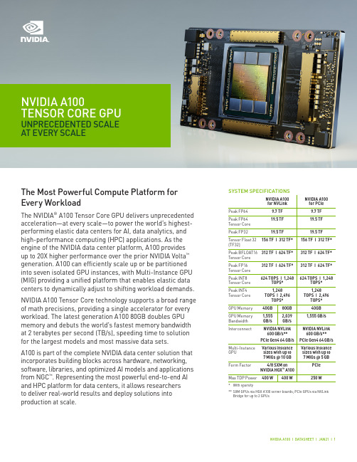
SYSTEM SPECIFICATIONSNVIDIA A100 for NVLinkNVIDIA A100 for PCIePeak FP649.7 TF 9.7 TF Peak FP64 Tensor Core 19.5 TF 19.5 TF Peak FP3219.5 TF 19.5 TF Tensor Float 32 (TF32)156 TF | 312 TF*156 TF | 312 TF*Peak BFLOAT16 Tensor Core 312 TF | 624 TF*312 TF | 624 TF*Peak FP16 Tensor Core 312 TF | 624 TF*312 TF | 624 TF*Peak INT8 Tensor Core 624 TOPS | 1,248 TOPS*624 TOPS | 1,248TOPS*Peak INT4 Tensor Core 1,248TOPS | 2,496TOPS*1,248TOPS | 2,496TOPS*GPU Memory 40GB 80GB 40GB GPU Memory Bandwidth 1,555 GB/s2,039 GB/s1,555 GB/s InterconnectNVIDIA NVLink 600 GB/s**PCIe Gen4 64 GB/s NVIDIA NVLink 600 GB/s**PCIe Gen4 64 GB/s Multi-Instance GPU Various instance sizes with up to 7 MIGs @ 10 GB Various instance sizes with up to 7 MIGs @ 5 GBForm Factor 4/8 SXM on NVIDIA HGX ™ A100PCIe Max TDP Power400 W400 W250 W* With sparsity** SXM GPUs via HGX A100 server boards; PCIe GPUs via NVLink Bridge for up to 2 GPUsNVIDIA A100TENSOR CORE GPUUNPRECEDENTED SCALE AT EVERY SCALEThe Most Powerful Compute Platform for Every WorkloadThe NVIDIA ® A100 Tensor Core GPU delivers unprecedented acceleration—at every scale—to power the world’s highest-performing elastic data centers for AI, data analytics, and high-performance computing (HPC) applications. As the engine of the NVIDIA data center platform, A100 provides up to 20X higher performance over the prior NVIDIA Volta ™ generation. A100 can efficiently scale up or be partitioned into seven isolated GPU instances, with Multi-Instance GPU (MIG) providing a unified platform that enables elastic data centers to dynamically adjust to shifting workload demands. NVIDIA A100 Tensor Core technology supports a broad range of math precisions, providing a single accelerator for every workload. The latest generation A100 80GB doubles GPU memory and debuts the world’s fastest memory bandwidth at 2 terabytes per second (TB/s), speeding time to solution for the largest models and most massive data sets. A100 is part of the complete NVIDIA data center solution that incorporates building blocks across hardware, networking, software, libraries, and optimized AI models and applications from NGC ™. Representing the most powerful end-to-end AI and HPC platform for data centers, it allows researchers to deliver real-world results and deploy solutions into production at scale.1X2X3XUp to 3X Higher AI Training on Largest Models DLRM TrainingUp to 249X Higher AI Inference Performance over CPUs BERT-LARGE InferenceGroundbreaking InnovationsNEXT-GENERATION NVLINKNVIDIA NVLink in A100 delivers 2X higher throughput compared to the previous generation. When combined with NVIDIA NVSwitch ™,up to 16 A100 GPUs can be interconnected at up to 600 gigabytes per second (GB/ sec), unleashing the highest application performance possible on a single server . NVLink is available in A100 SXM GPUs via HGX A100 server boards and in PCIe GPUs via an NVLink Bridge for up to 2 GPUs.efficiency at 95%. A100 delivers 1.7X highermemory bandwidth over the previous generation.to breakthrough acceleration for all their applications, and IT administrators can offer right-sized GPU acceleration for every job, optimizing utilization and expanding access to every user and application.STRUCTURAL SPARSITYAI networks have millions to billions of parameters. Not all of these parameters are needed for accurate predictions, and somecan be converted to zeros, making the models “sparse” without compromising accuracy. Tensor Cores in A100 can provide up to 2X higher performance for sparse models. While the sparsity feature more readily benefits AI inference, it can also improve the performance of model training.01X2XUp to 1.25X Higher AI Inference Performance over A100 40GB RNN-T Inference: Single StreamTime to Solution - Relative PerformanceCPU OnlyV100 32GBA100 40GBA100 80GBBig data analytics benchmark | 30 analytical retail queries, ETL, ML, NLP on 10TB dataset | CPU: Intel Xeon Gold 6252 2.10 GHz, Hadoop | V100 32GB, RAPIDS/Dask | A100 40GB and A100 80GB, RAPIDS/Dask/BlazingSQLUp to 1.8X Higher Performance for HPC Applications Quantum Espresso2017P1002016201820192020Throughput - Relative PerformanceGeometric mean of application speedups vs. P100: Benchmark application: Amber [PME-Cellulose_NVE], Chroma [szscl21_24_128], GROMACS [ADH Dodec], MILC [Apex Medium], NAMD [stmv_nve_cuda], PyTorch (BERT-Large Fine Tuner], Quantum Espresso [AUSURF112-jR]; Random Forest FP32 [make_blobs (160000 x 64: 10)], TensorFlow [ResNet-50], VASP 6 [Si Huge] | GPU node with dual-socket CPUs with 4x NVIDIA P100, V100, or A100 GPUs.Incredible Performance Across Workloads© 2021 NVIDIA Corporation. All rights reserved. NVIDIA, the NVIDIA logo, CUDA, DGX, HGX, HGX A100, NVLink, NVSwitch, OpenACC, TensorRT, To learn more about the NVIDIA A100 Tensor Core GPU, visit /a100The NVIDIA A100 Tensor Core GPU is the flagship product of the NVIDIA data center platform for deep learning, HPC, and data analytics. The platform accelerates over 1,800 applications, including every major deep learning framework. A100 is available everywhere, from desktops to servers to cloud services, delivering both dramatic performance gains and cost-saving opportunities.。

High Performance Approximate Sort AlgorithmUsing GPUsJun Xiao,Hao Chen,Jianhua SunCollege of Computer Science and Electronic EngineeringHunan UniversityChangsha,China*********************,******************,****************Abstract—Sorting is a fundamental problem in computer science,and the strict sorting usually means a strict order with ascending or descending.However,some applications in reality don’t require the strict ascending or descending order and the approximate ascending or descending order just meets the requirement.Graphics processing units(GPUs)have become accelerators for parallel computing.In this paper,based on the popular CUDA parallel computing architecture,we propose high performance approximate sort algorithm running on multicore GPUs.The algorithm divides the distribution interval of input data into multiple small intervals,and then uses the processing cores of GPUs to map the data into the different intervals in parallel. Finally by combining the small intervals,we can make the data between the different intervals in order state and the data in the same interval is disorder state.Thus we can get the approximate sorting result and the result is characterized by a general order but local disorder.By utilize the massive core of GPUs to parallel sort data,the algorithm can greatly shorten the execution time. Radix sort is the fastest GPUs-based sorting and the experimental results show that our approximate sort algorithm is two times as fast as the radix sort and far exceeds all the GPUs-based sorting. Keywords—sorting,parallel computing,high performance,GPUs, CUDAI.INTRODUCTIONSorting is one of most widely studied algorithmic problems in computer science,and has become a fundamental component in data structures and algorithms analysis.Many applications could be just classified as sorting problem,and the other applications depend on the efficient sorting as an intermediate step to accelerate the execution time[1],[2].For example,search engine widely uses of sorting to select valuable information to users.Therefore,designing and implementing efficient sorting routine is important on any parallel platforms.As many parallel platforms spring up,we need to explore efficient sorting techniques for utilizing parallel computing power[3].Recently,Graphics Processing Units have evolved into high performance accelerators and provide considerably higher peak computing and memory bandwidth than CPUs[4].For instance,NVIDIA’s GeForce GTX780GPUs contain up to 192scalar processing cores(SPs)per chip.And,these cores are broken up into12Streaming Multiprocessors(SMs)and each SM comprises16SPs.A3GB off-chip global memory is shared by the192on-chip cores.By introduction of CUDA, programmers could use C to program GPUs for general-purpose computation[5].In consequence,it is an explosion of research on GPUs for high performance computing[6].With the high computing power,advanced features such as atomic operations,shared memory and synchronization,also lead into modern GPUs.Many researchers have proposed GPUs-based sorting algorithms and transit from the coarse-grained parallelism of multicore chips to the fine-grained parallelism of manycore chips.Quick sort is a popular sorting algorithm,and Cederman et al.[7]have adapted quick sort for GPUs to parallelization. Satish et al.[3]have designed efficient sorting algorithms to make use of the fast on-chip memory provided by NVIDIA GPU and change from a largely task-parallel structure to a more data-parallel structure.The studies of GPUs sorting mainly concentrate on bitonic sort,quick sort,radix sort and merge sort.However,these GPUs-based sorting are belong to the strict sorting.The strict sorting usually means the strict order with ascending or descending after sorting.Some applications in the reality don’t necessarily require the strictly ascending or descending order,and tolerate unsorted order to some extent. As a result,the approximately ascending or descending order already meets the requirement.In this situation,the overhead of the strict sorting is relatively high.Our focus,in this paper,is to develop the approximate sort on manycore GPUs which is suitable for sorting data to reach the state of the approximately ascending or descending order. Our experimental results demonstrate that our approximate sort is fastest in all previously published GPUs sorting when running on current-generation NVIDIA GPUs.The radix sort is the fastest GPUs sorting for the large amount data[3]and our approximate sort could achieve at least more than twice compared with GPUs-based radix sort.The rest of this paper is organized as follows:In Section2 we will describe the background on GPUs architecture and the sorting on GPUs.In Section3we will elaborate the approximate sort in detail.In Section4we will present theInternational Conference on Computer Science and Intelligent Communication (CSIC 2015)experimental evaluation of the approximate sort compared with GPUs-based sorting.II.BACKGROUNDIn this section,we will provide background information on GPU architecture and the GPU-based sorting.A.GPUs architectureOur approximate sort algorithm is designed and implemented on the NVIDIA GPUs architecture.GPUs have become high performance accelerators for parallel computing, which are massively multi-threaded data-parallel processor. GPUs contain two major components:the processing component and the memory component.A certain number of streaming multiprocessors comprises the processing component.At the same time,each streaming multiprocessor includes a series of simple cores that execute the in-order instructions.For high performance,a few tens of thousands of threads are launched and these threads carry out the same instruction on the different data sets.Threads in GPUs have three-level hierarchy:each block includes hundreds of threads mapped to a streaming multiprocessor and a grid contains a set of blocks executed on a kernel[8].In the memory component,the off-chip global memory in GPUs is accessible across all streaming multiprocessors.The data transfer between host and device memory is at the means of DMA.A16KB on-chip cache equipped in each streaming multiprocessor,which has very high bandwidth and very low access latency.Our approximate sort algorithm leverages the CUDA Data Parallel Primitives library[9],specifically its scan and reduce. By using the CUDPP library,we avoid do tedious work that the CUDPP has done for us.B.Sorting on GPUsWe here present only the most relevant work because sorting on GPUs has always been the research hotspot.Early GPUs-based sorting algorithms were primarily based on Batcher’s bitonic sort[10].Barajlia et al.[11]presented a practical bitonic sorting network implemented in CUDA when bringing in the new general-purpose parallel platform. Cederman et al.[7]developed an efficient implementation of GPUs quick sort to make use of the highly parallel nature and its limited cache memory.Satish et al.designed efficient parallel radix sort and merge sort for GPUs,and their radix sort is the fastest GPU sort[3].Above mentioned sorting can be viewed as a feasible alternative to sort a large amount of data on GPUs.However, these sorting routines are all belong to the strict sorting.We define the strict sorting that the strict order with ascending or descending after sorting,otherwise call as the approximate sorting.For example,we have an input array of(10,8,2,9,3, 1)and sort in ascending order.If the output is(1,2,3,8,9,10) with strict order,the sorting algorithm used is part of the strict sorting.If the output is(1,3,2,10,9,8)or others with unsorted within the interval and sorted between the intervals,the sorting algorithm used belongs to the approximate sorting. The length of the interval controlled by the users and the length of the interval is3in this case.For further explanation, (1,3,2)and(10,9,8)are two intervals.(1,3,2)or(10,9,8)is unsorted but every element in(1,3,2)is less than the one in (10,9,8),that is the ascending order between the intervals and it means the approximately ascending order.Some applications in the reality don’t necessarily require the strictly ascending or descending order,and tolerate unsorted order to some extent.As a result,the approximately ascending or descending order already meets the requirement. In this situation,the overhead of the traditional sorting is relatively high.We propose lightweight approximate sort on manycore GPUs to address the above problem.III.APPROXIMATE SORT ON GPUS In the following section,we present the detail of approximate sort algorithm on GPUs to parallelism.Fig.1.Illustration of approximate sort on GPUs As shown in Figure1,our algorithm on GPUs operates in three steps.First,each data element in the input array is mapped into a smaller interval(the number of the smaller intervals is a pre-defined parameter and typically much less than the input size,NUM_INTERVAL=3in our case).In this step,we use offset array to maintain an ordering among all data elements that are mapped into the same interval.At the same time,the interval counter array is use to record the number of data elements falling into each interval.Second,an exclusive prefix sum operation is performed on the interval counter array.In the third step,the results of the above two steps are combined to produce the final coordinates that are then used to transform the input array to the approximately-sorted form.Step1:Similar to many parallel sort algorithms that subdivide the input into the equally-sized intervals and then sort each interval in parallel,we first map each data element of the input array into an interval.As shown in Listing1,the number of the interval is a fixed value NUM_INTERV AL,and the mapping procedure is a linear projection of each data element of the input vector to one of the NUM_INTERV ALintervals.The linear projection is demonstrated at lines10and 11in Listing1.The variables of min and max represent the minimum and maximum value in the input respectively,which can be obtained when using the CUDPP’s reduce tool on GPUs.In this way,each interval represents a partition of the interval[min,max],and all intervals have the same width of (max-min)/NUM_INTERVAL.The data elements in the input array are assigned to the target interval whose value range contains the corresponding data element,and for brief illustration we use interval_index array to record the target interval.In addition,another array interval_count is maintained to record the number of data assigned to each interval.As shown at line13,the offset array is based on an atomic function provided by CUDA,atomicInc,to avoid the potential conflicts incurred by concurrent writes.The function atomicInc returns the old value located at the address presented by its first parameter,which can be leveraged to indicate the local ordering among all the data elements assigned to the same interval.The Kepler GPUs have substantially improved the throughput of atomic operations compared to Fermi GPUs,which also demonstrated in our implementation.1__global__void assign_interval(uint∗input,uint lenght,uint max,uint min,2uint∗offset,uint∗interval_count,uint∗interval_index) 3{4int idx=threadx.x+blockDim.x∗blockIdx.x;5uint interval_idx;6for(;idx<lenght;idx+=total_threads)7{8uint value=input[idx];910interval_idx=(size−min)∗(NUM_INTERVAL−1)/(max−min);11interval_index[idx]=interval_idx;1213offset[idx]=atomicInc(&interval count[interval_idx],length);14}15}1__global__void appr_sort(uint∗key,uint∗key_sorted,void∗value,uint length,2void∗value_sorted,uint∗offset,uint∗interval_count, 3uint∗interval_index)4{5int idx=threadIdx.x+blockDim.x∗blockIdx.x;6uint count=0;7for(;idx<length;idx+=total threads)8{9uint Key=key[idx];10uint Value=value[idx];1112uint Interval_index=interval_index[idx];13count=interval_count[Interval_index];14uint off=offset[idx];15off=off+count;1617key_sorted[off]=key;18value_sort[off]=value;19}20}Step2:Having obtained the counters for each interval and the local ordering within a specific interval,we perform a prefix sum operation on the interval_count array to determine the address at which each interval’s data would start.Given an input array,the prefix sum,also known as scan,is to generate a new array B from original array A in which each data B[i]is the sum of data from A[0]to A[i](inclusive and exclusive prefix sum respectively).Because the length of the interval count_array(NUM_INTERV AL)is typically less than that of the length of the input,performing the scan operation on CPU is much fast than the GPUs counterpart.However,due to the data transfer overhead(in our case,two transfers),and the fact that we observed devastating performance degradation when mixing the execution of the CPU-based scan with other GPUs kernels in a CUDA stream,the parallel prefix sum is performed on GPUs using the CUDPP library.Step3:By combining the atomically-incremented offsets generated in step1and the interval data locations produced by the prefix sum in step2(as shown at lines12-15in Listing2), it is straightforward to scatter the key-value pairs to proper locations(see lines17-18).Choosing a suitable value for the number of intervals may have important implications for the efficiency and effectiveness of our sorting algorithm.As the number of intervals increases,if the input data exhibiting uniform distribution of elements,our algorithm would approximate more closely to the ideal sorting,while the overhead of performing the prefix sum may increase accordingly.When decreasing the number of intervals,we will get a coarse-grained approximation for the input array.We will present empirical evaluations on this in Section IV.IV.EXPERIMENTAL EVALUATIONA.Experiment setupWe ran the experiments on an eight-processor Intel Xeon E52648L1.8GHz machine.At the same time,the machine equipped with a high-end NVIDIA GeForce GTX780GPUs with12multiprocessors and192GPUs processing cores.We compared approximate sort on GPUs with the following state-of-the-art GPUs sorting algorithms:Satish et al.’s[3]merge sort and radix sort.Because the version of radix sort is the fastest GPUs sort and the version of merge sort is the fastest comparison-based GPUs sort according to the reference.At the same time,the source code of that merge sort and radix sort is available in the NVIDIA CUDA SDK[12].The data sets we automatically generated for the benchmark test conform to Uniform distribution or Gaussian distribution.Values that are picked randomly from0to231 produce Uniform distribution.The Gaussian distribution is created by always taking the average of four randomly picked values from the uniform distribution[7].We choose the two distributions for the representative.B.Performance analysisWe compare our approximate sort with merge sort and radix sort on GPUs.First,we generate respectively three data sets on Uniform distribution and Gaussian distribution.The size of the data set we evaluate is1M,2M,4M(M means106in this paper)and we set the NUM_INTERV AL =10000.As shown in Figure 2and Figure 3,the performance on the two distributions is roughly the same.When the data volume is doubling,the cost of approximate sort slowly increases compared with merge sort.Our approximate could achieve at least more than twice compare with radixsort.Data SizeFig.2.Data sets on UniformdistributionData SizeFig.3.Data sets on Gaussian distributionFig.4.The parameter of NUM_INTERV ALIn the Figure 4,we evaluate how the parameter of NUM_INTERV AL effects on performance.We prepare two data set on Uniform distribution and the size of the data set respectively 1M and 2M.The values of NUM_INTERVAL is (10000,20000,30000,40000,50000,60000,70000,80000,90000).As the NUM_INTERVAL increased,the executiontime of approximate sort almost the same.When the NUM_INTERVAL is small,the cost of atomic operation is high because multiple elements are assigned to the same interval concurrently and the overhead of prefix sum is small.When the NUM_INTERVAL is large,the cost of atomic operation is low because fewer elements are assigned to the same interval concurrently but the overhead of prefix sum is expensive.It is suggested that the performance almost keep same when the NUM_INTERV AL changes within a certain range.V.CONCLUSIONSThis paper,we propose approximate sort on manycore GPUs to parallelism.The approximate sort could obtain the approximate order with ascending or descending by controlling the parameter of NUM_INTERVAL.The radix sort is the fastest GPUs sort and our approximate sort could achieve at least more than twice compared with GPUs-based radix sort.As for future,our work is to integrate our approximate sort into the application in the reality.VI.ACKNOWLEDGMENTThis research was supported in part by the National Science Foundation of China under grants 61272190and 61173166,the Program for New Century Excellent Talents in University,and the Fundamental Research Funds for the Central Universities of China.REFERENCES[1]D.E.Kauth,“The art of computer programming:Volume 3/sorting and searching,”1973.[2]T.H.Cormen,C.E.Leiserson,R.L.Rivest,C.Stein et al.,Introductionto algorithms.MIT press Cambridge,2001,vol.2.[3]N.Satish,M.Harris,and M.Garland,“Designing efficient sortingalgorithms for manycore gpus,”in Parallel &Distributed Processing,2009.IPDPS 2009.IEEE International Symposium on.IEEE,2009,pp.1–10.[4] C.Nvidia,“Nvidia cuda c programming guide,”NVIDIA Corporation,vol.120,2011.[5]J.Nickolls,I.Buck,M.Garland,and K.Skadron,“Scalable parallelprogramming with cuda,”Queue,vol.6,no.2,pp.40–53,2008.[6]S.Bandyopadhyay and S.Sahni,“Grsgpu radix sort for multifieldrecords,”in High Performance Computing (HiPC),2010International Conference on.IEEE,2010,pp.1–10.[7] D.Cederman and P.Tsigas,“A practical quicksort algorithm forgraphics processors,”in Algorithms-ESA 2008.Springer,2008,pp.246–258.[8]L.Chen and G.Agrawal,“Optimizing mapreduce for gpus witheffective shared memory usage,”in Proceedings of the 21st international symposium on High-Performance Parallel and Distributed Computing.ACM,2012,pp.199–210.[9]M.Harris,J.Owens,S.Sengupta,Y.Zhang,and A.Davidson,“Cudpp:Cuda data parallel primitives library,”2007.[10]K.E.Batcher,“Sorting networks and their applications,”in Proceedingsof the April 30–May 2,1968,spring joint computer conference.ACM,1968,pp.307–314.[11]R.Baraglia,G.Capannini,F.M.Nardini,and F.Silvestri,“Sortingusing bitonic network with cuda,”in the 7th Workshop on Large-Scale Distributed Systems for Information Retrieval (LSDS-IR),Boston,USA,2009.[12]“Nvidia cuda sdk,”(/cuda),2014.。

AI计算系统选择FPGA的六大疑惑与解答这几天,已经退役的AlphaGo又强行刷了一波头条,不是又跟哪位世界高手对决,而是“新狗”通过无监督式学习,仅用3天时间就战胜了李世石版的AlphaGo,然后用了21天时间战胜了柯洁版本AlphaGo。
AlphaGo让我们真真切切地看到了AI计算的强大。
目前,在AI计算平台使用最广泛的两种加速部件是GPU和FPGA。
GPU可适用于具备计算密集、高并行、SIMD(Single Instruction Multiple Data,单指令多数据流)应用等特点的深度学习训练模型领域,并且GPU创建了包含CNN、DNN、RNN、LSTM以及强化学习网络等算法在内的应用加速平台和生态系统。
但是,最近FPGA又频频被各AI领域的巨头看好,比如微软、百度、科大讯飞都对FPGA 应用前景有所期待。
那么如果让你选择FPGA作为AI计算系统的主力军,你会有什么样的顾虑?顾虑一:FPGA有啥优势?什么样的场景更适合FPGA?首先,深度学习包含两个计算环节,即训练和推理环节。
GPU在深度学习算法模型训练上非常高效,但在推理时对于小批量数据,并行计算的优势不能发挥出来。
而FPGA 同时拥有流水线并行和数据并行,因此处理任务时候延迟更低。
例如处理一个数据包有10 个步骤,FPGA 可以搭建一个10 级流水线,流水线的不同级在处理不同的数据包,每个数据包流经10 级之后处理完成。
每处理完成一个数据包,就能马上输出。
通常来说,FPGA 加速只需要微秒级的PCIe 延迟。
当Intel 推出通过QPI快速通道互联的Xeon + FPGA 之后,CPU 和FPGA 之间的延迟甚至可以降到100 纳秒以下。
其次,FPGA是可编程芯片,算法烧录更加灵活。
目前来看,深度学习算法还未完全成熟,算法还在迭代衍化过程中,若深度学习算法发生大的变化,FPGA是软件定义硬件,可以灵活切换算法,快速切入市场。
未来至少95%的机器学习计算都是用于推断,只有不到5%是用于模型训练,而FPGA正。

基于PCIe高速通信接口的图像处理系统设计袁柳; 李皓; 李勐; 涂吉【期刊名称】《《科学技术与工程》》【年(卷),期】2019(019)022【总页数】6页(P235-240)【关键词】PCIe; 现场可编程门陈列(FPGA); 图像处理; 手写字符识别; 卷积神经网络【作者】袁柳; 李皓; 李勐; 涂吉【作者单位】中国电子科技集团公司电子科学研究院北京100041; 武汉大学电子信息学院武汉430072【正文语种】中文【中图分类】TP391.41随着大数据、人工智能行业的发展,图像、视频等所需处理的数据量呈爆炸性增长,尤其在以卷积神经网络(convolutional neural network,CNN)为代表的深度学习领域,图像处理系统的计算能力和传输能力需要不断提高。
传统的中央处理器(central processing unit,CPU)、图形处理器(graphics processing unit, GPU)架构存在能耗高、性价比低等问题,现场可编程门陈列(field-programmable gate array,FPGA)作为可编程的硬件,可以根据应用需要实现硬件动态重构,具备高度并行的流水处理能力,CPU+FPGA异构处理架构正成为图像处理的重要解决方案之一[1]。
CPU和FPGA之间高效协同处理需要高速数据传输接口,PCIe总线支持基于PCIe Switch芯片的接口扩展,支持接口位宽、接口数量动态配置,具备优异的可扩展性、灵活性、普适性和低延迟特性,文献[2—5]通过PCIe DMA技术可以实现CPU和FPGA之间的高速数据通信,但是由于PCIe接口复杂,需要丰富的设计经验,目前基于 PCIe接口的图像处理系统还没有得到广泛推广。
文献[6—9]开始借助PCIe高速通信接口实现多路视频图像传输,但是还没有形成一种统一的基于PCIe 的图像处理框架,需要根据不同应用从头开始设计FPGA硬件架构,导致应用开发效率不高。

Arbitrary Function GeneratorsAFG31000 Series DatasheetThe Tektronix AFG31000 Series is a high-performance AFG with built-in arbitrary waveform generation, real-time waveform monitoring, and the largest touchscreen on the market. Providing advanced waveform generation and programming capabilities, waveform verification, and a modern touch-screen interface, the new AFG31000 is sure to delight and simplify the job of every researcher and engineer.Key performance specifications1 or2 channel modelsOutput amplitude range 1 mV P-P to 10 V P-Pinto 50 Ω loadsBasic (AFG) mode:25 MHz, 50 MHz, 100 MHz, 150 MHz, or 250 MHz sine waveforms250 MSa/s, 1 GSa/s or 2 GSa/s sample rates14-bit vertical resolutionBuilt-in waveforms include sine, square, ramp, pulse, noise, andother frequently used waveformsSweep, Burst, and Modulation modes (AM, FM, PM, FSK, andPWM)Advanced (Sequence) mode:Continuous mode (optional Sequence, Triggered and Gatedmodes)16 Mpts arbitrary waveform memory on each channel (128 Mptsoptional)Up to 256 steps in sequence mode with loop, jump and wait events Variable sampling clock 1 µSa/s to 2 GSa/sKey featuresPatented InstaView ™ technology enables engineers to see the actual waveform at the Device Under Test (DUT) in real time, without the need of an oscilloscope and probe, eliminating the uncertainty causedby mismatched impedanceSequencing option adds the ability to program long, complexwaveforms with up to 256 stepsThe 9-inch capacitive touch screen works like a smart phone and hasshort-cuts to frequently used settingsBuilt-in ArbBuilder lets you create and edit arbitrary waveforms on theinstrument, eliminating the need to connect to a PCOutputs are protected from over voltage and current to minimizepotential instrument damageCompatible with TekBench ™ software to help students set up, control,and analyze test results in the labApplicationsAdvanced researchClock and system synchronizationReplication of real world signalsComponent and circuit characterization and validationEmbedded circuit design and testGeneral purpose signal generationBasic and Advanced ModesThe AFG31000 series is the industry’s first arbitrary function generator with full function Basic (AFG) and Advanced (Sequence) modes.In Basic mode, the AFG31000 generates traditional functions and arbitrary waveforms. The touchscreen and front-panel controls make it simple to set up.Basic mode lets you change frequency without the need to worry about waveform length and sample rate. This feature is useful in analog designs that characterize filter/amplifier frequency responses or in digital designs where clock rates change frequently.Key settings are visible at a glance, and are easy to adjust using touch, numeric keypad, or rotary controlsNew with the AFG31000, Advanced mode provides the ability to generate multiple waveforms with complex timing. In this mode, you can compose a list (or a sequence) of 1 to 256 waveforms, with total waveform length up to 16 Mpts/ch (128 Mpts/ch optional) and define the ouput sequence of these waveforms. Repeat, go-to, wait, jump, and triggered events are all supported and the large memory provides space to store many waveforms or long waveforms.This feature is very useful in applications where many test cases need to be performed sequentially. Instead of loading the test cases one by one, you can put all of them in a sequence and load at one time, switching from one to another seamlessly to greatly improve the test efficiency.Advanced mode lets you build complex waveform sequences with flexible step controlsSequenced sine waveforms with different frequency and amplitude. Additionally, Advanced mode uses variable sample rate technology. Every sample in a waveform is output once and only once in each cycle, synchronized to the sample rate. Since there is no skipping or repetition, all details in the waveforms are kept. This feature is very useful for applications in which signal fidelity is extremely critical, such as IQ modulation and pulse train generation.InstaView™ technology shows the actual waveform at the DUTMost waveform generators assume they are driving a 50 Ω impedance. However, most devices under test do not have a 50 Ω impedance. This mismatch results in an inconsistency between the waveform as set on the AFG and the signal at the DUT.DatasheetWith InstaView turned off, the AFG31000 works like a traditional function generator. Due to an impedance mismatch, the AFG display shows a different waveform from the one observed at the DUT.With the patented InstaView ™technology, the AFG31000 Series can display the actual waveform at the DUT, instead of just the nominalwaveform as set on the AFG. The waveform displayed on the AFG instantly responds to changes in frequency, amplitude, waveform shape, andimpedance changes at the DUT. InstaView helps eliminate the uncertainty and measurement risk caused by impedance mismatches, without requiringadditional cables, instruments, or effort.With InstaView turned on, the AFG31000 shows the waveform as observed at the DUT.A large touch screen and smart user interfaceThe large 9-inch capacitive touch screen displays all related settings and parameters on a single screen. Similar to smart devices, you can tap or swipe to easily select, browse, locate and change settings and parameters.Frequently-used functions are immediately accessible. Familiar buttons and rotary knob controls are available for more traditional navigation.Frequently used settings are easy to access from the swipe-up menuAFG31000 SeriesBuilt-in ArbBuilder tool makes creating and editing arbitrary waveforms easier than ever In the past, you needed a PC with waveform editing software to create or edit your arbitrary waveforms. The waveform would then need to be downloaded to the AFG using either a USB stick or a data cable connection. The process was time-consuming, especially when waveforms required frequent changes.ArbBuilder is a built-in application on the AFG31000 series that lets you create and edit your arbitrary waveforms directly on the generator. You can create arbitrary waveforms with the Equation Editor tool or start from a library of standard templates. Thanks to the large capacitive touch screen, you can drag, pinch and zoom to get the detail you need.You can quickly replicate real-world waveforms captured with oscilloscopes or created by third-party software by loading CSV format data files directly into ArbBuilder from a USB memory stick.Creating an arbitrary waveform using the easy touch screen interfaceSimplified multi-unit synchronizationMost applications need one or two channels of output, but some applications require more channels. For example, in order to simulate 3-phase power signals, engineers often need to synchronize three 2-channel generators; one for the voltage and current on each phase. To do this used to be time-consuming, as it required many cable connections between the AFG units, and making changes in deep branches of the menu trees on all instruments.The AFG31000 simplifies this process with an onscreen wizard that leads you through the process of making cable connections and configuring settings to synchronize multiple generators.An on-screen wizard guides you through the process of multiple-unit synchronizationUpgradability protects your investmentThe AFG31000 provides upgrade options for bandwidth, memory extension, and sequence mode support. These options can be installed at the factory or at any time after purchase. This upgradability helps to reduce the product ownership threshold. And when your test requirements change, you can purchase and install upgrade software licenses to add higher performance features. Upgrades eliminate the concern about the return on investment during the instrument lifetime.DatasheetAFG31000 SeriesSpecificationsAll specifications are guaranteed unless noted otherwise. All specifications apply to all models unless noted otherwise.Model overviewOutput characteristicsAmplitudeOutput impedance50 ΩLoad impedance setting Selectable: 50 Ω, 1 Ω to 10.0 kΩ, High Z (Adjusts displayed amplitude according to selected load impedance)Isolation42 Vpk maximum to earth groundShort-circuit protection Signal outputs are robust against permanent shorts against floating groundOvercurrent protection When incoming current is greater than 250 mA, the output channels are protected with relays that disconnect the AFG from thedevice under test. Connection can be resumed by user after removing the incoming currentGeneral characteristics - Basic modeBasic (AFG)Run modes Continuous, Modulation, Sweep and BurstStandard waveforms Sine, Square, Pulse, Ramp, More (Noise, DC,Sin(x)/x, Gaussian, Lorentz, Exponential Rise, Exponential Decay, Haversine )Arbitrary waveformsSampling clock: 250 MSa/s, 1 GSa/s or 2 GSa/s (model and waveform length apply)Vertical resolution: 14 bitsWaveform length: 2 to 131,072 pointsSineFrequency rangeEffective maximum frequency outAmplitude flatness (1 V P-P ,relative to 1 kHz)Amplitude flatness (1 V P-P ,relative to 1 kHz), typicalHarmonic distortion (1 V P-P ),typicalDatasheetTHD, typical≤ 0.04%, 10 Hz to 20 kHz, 1 V P-PSpurious noise (1 V P-P ), typicalPhase noise, typical< -125 dBc/Hz at 20 MHz, 10 kHz offset, 1 V P-PResidual clock noise, all models -63 dBmSquareFrequency rangeRise/fall time, typicalOvershoot, typical< 3%Jitter (RMS), typical2.5 psRampFrequency rangeLinearity, typical (1 kHz, 1 V P-P ,100% symmetry)Symmetry0% to 100%AFG31000 SeriesGeneral characteristics - Basic modePulseFrequency rangePulse widthPulse width resolution 10 ps or 5 digitsPulse Duty 0.001% to 99.999% (limitations of pulse width apply)Edge transition timeEdge transition time resolution 10 ps or 4 digits Lead delay rangeLead delay resolution 10 ps or 8 digits Overshoot, typical < 2%Jitter (RMS), typical 2.5 psDCRange (into 50 Ω)Resolution (into 50 Ω) 1 mV or 4 digits Accuracy ± (1% of |setting | +1mV)NoiseBandwidth (-3 dB)Noise typeWhite GaussianInternal noiseDatasheetGeneral characteristics - Basic modeOther waveformsFrequency rangeArbitrary waveformsFrequency rangeEffective analog bandwidth (-3 dB)Waveform length2 to 131,072Sample rateVertical resolution14 bitRise/fall time, typicalJitter (RMS), typical2.5 psModulationAM, FM, PMAM modulation depth0.0 % to 120 %AM modulation resolution0.1%AFG31000 SeriesGeneral characteristics - Basic modeMinimum FM peak deviationDCMaximum FM peak deviationPM phase deviation range0° to 180°PM phase resolution0.1°FSKPWMSweepType Linear, Logarithmic Waveforms All, except Pulse, Noise, DC Sweep time 1 ms to 500 s Hold/return time0 s to 500 s Maximum total sweep time500 sAccuracy, typical: ≤ 0.4%Minimum start/stop frequency All except ARB: 1 μHzARB: 1 mHzMaximum start/stop frequencyDatasheetGeneral characteristics - Basic modeBurstWaveform All except Noise, DC Type Triggered, gatedBurst count 1 to 1,000,000 cycles or Infinite Intenal trigger rate 1 μs to 500.0 sGate and trigger sources Internal, external, remote interfaceInstaView ™Waveforms All except noise Cable (channel output to load)50 Ω BNC to BNCRun modeContinuous in Basic modeMaximum measurement range (DC + peak AC voltage)DC level measurementAmplitude measurementBandwidth (-3 dB)500 MHzFlatness, sine, 1 V P-P , into 50 ohm, relative to 1 kHz,typicalCable propagation delay measurement, typicalAFG31000 SeriesGeneral characteristics - Basic modeGeneral characteristics - Advanced modeWaveform memory size 16 Mpts (128 Mpts optional) each channel Run modeStandard: ContinuousOptional: Sequence, Triggered, GatedNumber of waveform entriesContinuous, Triggered, Gated: 1 Sequence: 1 to 256Minimum waveform length 168 pts Waveform granularity 1 pt Vertical resolution 14 bitsJump/trigger events External trigger (rising or falling edge), manual trigger, timer, SCPI commands Repeat count 1 to 1,000,000 or infinite Timer range 2 µS to 3600 S Timer resolution 4 ns or 8 digitsVariable sample rateRise/Fall time, typicalOvershoot, typical< 2%Level flatness, typical (sine, 1 V P-P ,relative to 1 kHz)Harmonic distortion, typical (sine with 64 pts/cycle, 1 V P-P )DatasheetSpurious, typical (sine with 64 pts/cycle, 1 V P-P )Spurious free dynamic range,typical (sine with 64 pts/cycle,1 V P-P )Phase noise, typical (sine with 64 pts/cycle, 1 V P-P , at 10 kHz offset)Skew controlRange -320 ns to 320 ns (channel 1 to channel 2 on dual channel models, at maximum sample rate)Resolution 100 ps or 4 digits Accuracy, typical ±(1% of |setting| + 500 ps)Initial skew, typical< 500 psSystem characteristicsOutput Frequency ResolutionFrequency accuracy±10-6 of setting (all except ARB), 0 °C to 50 °C (32 °F to 122 °F)±10-6 of setting ± 1 μHz (ARB), 0 °C to 50 °C (32 °F to 122 °F)Aging ±1.0 x 10⁻⁶ per yearPhaseRange -180° to +180°Resolution0.01° (sine)0.1° (other waveforms)Remote program interface GPIB, Ethernet 10BASE-T / 100BASE-TX / 1000BASE-T, USB 2.0Maximum configuration times,typicalPower sourceSource100-240 V, 47-63 Hz 115 V, 360-440 HzConsumption120 WAFG31000 SeriesGeneral characteristics - Advanced modeWarm up time, typical 20 minutes minimum Power on self diagnosis time < 24 s Acoustic noise < 50 dBADisplay9-inch capacitive touch screen with 800 * 480 resolutionUser interface and Help languages English, French, German, Japanese, Korean, Simplified and Traditional Chinese, Russian (user selectable)Auxiliary input characteristicsExternal modulation input, channel 1 and channel 2Input rangeInput impedance 5.2 kΩFrequency range 125 kHz (1 MSa/s)External Trigger inputLevel TTL compatible Impedance10 kΩMinimum pulse width 100 nsSlopePositive or negative selectable Trigger delay range 0 ns to 85 s Trigger delay resolution 100 ps or 5 digitsTrigger latency, typical 390 ns (trigger input to signal output)Jitter (RMS), typical 100 ps (signal output, with external trigger input in burst mode)10 MHz reference clock inputImpedance 1 kΩInput couplingACRequired input voltage swing 100 mV P-P to 5 V P-P Lock range10 MHz ±35 kHz Channel 1 external add inputImpedance 50 ΩInput range -1 V to +1 V (DC + peak AC)BandwidthDC to 10 MHz (-3 dB) at 1 V P-P DatasheetSystem characteristicsAFG31000 Series Auxiliary output characteristicsChannel 1 trigger outputLevel Positive TTL level pulse into 1 kΩImpedance50 ΩJitter, RMS, typical10 ps for all modelsOutput frequency10 MHz reference clock outImpedance50 Ω, AC coupledAmplitude 1.2 V P-P into 50 Ω loadPhysical characteristicsDimensionsHeight191.8 mm (7.55 in.)Width412.8 mm (16.25 in.)Depth143.3 mm (5.64 in.)WeightNet 4.7 kg (10.4 lb.)Shipping7.0 kg (15.4 lb.)EMC, environment, and safetyTemperatureOperating0 °C to +50 °C (32 °F to 122 °F)Nonoperating-30 °C to +70 °C (-22 °F to 158 °F)HumidityOperating≤ 80%, 0 °C to 40 °C (32 °F to104 °F)≤ 60%, > 40°C to 50°C (104 °F to 122 °F), noncondensingNonoperating5% to 90%, < 40 °C (< 104 °F), noncondensing5% to 80%, ≥ 40 °C to 60 °C (≥ 104 °F to 140 °F), noncondensing5% to 40%, > 60 °C to 70 °C (> 140 °F to 158 °F), noncondensingAltitudeOperating Up to 3,000 m (9,842 ft.)Nonoperating Up to 12,000 m (39,370 ft.)EMC compliance EN61326-1:2013, EN 61326-2-1:2013European Union EU Council Directive 2004/108/ECDatasheetEMC, environment, and safetySafety UL 61010-1:2004CAN/CSA C22.2 No. 61010-1:2004IEC 61010-1:2001Over-temperature protection Instrument is protected from over-temperature by turning off outputsAFG31000 Series Ordering InformationModelsAFG31021 1 μHz to 25 MHz sine wave, 1-channel arbitrary function generatorAFG31022 1 μHz to 25 MHz sine wave, 2-channel arbitrary function generatorAFG31051 1 μHz to 50 MHz sine wave, 1-channel arbitrary function generatorAFG31052 1 μHz to 50 MHz sine wave, 2-channel arbitrary function generatorAFG31101 1 μHz to 100 MHz sine wave, 1-channel arbitrary function generatorAFG31102 1 μHz to 100 MHz sine wave, 2-channel arbitrary function generatorAFG31151 1 μHz to 150 MHz sine wave, 1-channel arbitrary function generatorAFG31152 1 μHz to 150 MHz sine wave, 2-channel arbitrary function generatorAFG31251 1 μHz to 250 MHz sine wave, 1-channel arbitrary function generatorAFG31252 1 μHz to 250 MHz sine wave, 2-channel arbitrary function generatorOptionsFactory optionsMEM Extends arbitrary waveform memory to 128 Mpts/ch in Advanced modeSEQ Enables Sequence, Triggered and Gated modes in Advanced modeFeature upgrade after purchaseThe AFG31000 products offer several ways to easily add functionality after the initial purchase.DatasheetPower plug optionsOpt. A0North America power plug (115 V, 60 Hz)Opt. A1Universal Euro power plug (220 V, 50 Hz)Opt. A2United Kingdom power plug (240 V, 50 Hz)Opt. A3Australia power plug (240 V, 50 Hz)Opt. A5Switzerland power plug (220 V, 50 Hz)Opt. A6Japan power plug (100 V, 50/60 Hz)Opt. A10China power plug (50 Hz)Opt. A11India power plug (50 Hz)Opt. A12Brazil power plug (60 Hz)Opt. A99No power cordLanguage optionsOpt. L0English front panel overlay (default)Opt. L1French front panel overlayOpt. L2Italian front panel overlayOpt. L3German front panel overlayOpt. L4Spanish front panel overlayOpt. L5Japanese front panel overlayOpt. L6Portuguese front panel overlayOpt. L7Simplified Chinese front panel overlayOpt. L8Traditional Chinese front panel overlayOpt. L9Korean front panel overlayOpt. L10Russian front panel overlayOpt. L99No front panel overlayService optionsOpt. C3Calibration Service 3 YearsOpt. C5Calibration Service 5 YearsOpt. D1Calibration Data ReportOpt. D3Calibration Data Report 3 Years (with Opt. C3)Opt. D5Calibration Data Report 5 Years (with Opt. C5)Opt. R5Repair Service 5 Years (including warranty)Opt. T3Three Year Total Protection Plan, includes repair or replacement coverage from wear and tear, accidental damage, ESD or EOSplus preventative maintenance. Including a 5 day turnaround time and priority access to customer support Opt. T5Five Year Total Protection Plan, includes repair or replacement coverage from wear and tear, accidental damage, ESD or EOSplus preventative maintenance. Including a 5 day turnaround time and priority access to customer supportAccessories are not covered by the instrument warranty and Service Offerings.AccessoriesStandard accessories-----AFG31000 Series Arbitrary Function Generator Compliance, Installation, and Safety Instructions 012-1732-xx BNC cable shielded, 3 ft.174-4401-xx USB cable, A to B, 3 ft.-----Power cord-----NIST-traceable calibration certificate-----Three-year warranty on parts and laborRecommended accessories012-1732-xx BNC cable shielded, 3 ft.012-0991-xx GPIB cable, double shielded011-0049-02 50 Ω BNC terminatorACD4000B Soft transit caseHCTEK54Hard transit case (requires ACD4000B)WarrantyProduct warranty Three-year warranty on parts and laborTektronix is registered to ISO 9001 and ISO 14001 by SRI Quality System Registrar.Product(s) complies with IEEE Standard 488.1-1987, RS-232-C, and with Tektronix Standard Codes and Formats.Product Area Assessed: The planning, design/development and manufacture of electronic Test and Measurement instruments.AFG31000 SeriesDatasheetASEAN / Australasia (65) 6356 3900 Austria 00800 2255 4835*Balkans, Israel, South Africa and other ISE Countries +41 52 675 3777 Belgium 00800 2255 4835*Brazil +55 (11) 3759 7627 Canada180****9200Central East Europe and the Baltics +41 52 675 3777 Central Europe & Greece +41 52 675 3777 Denmark +45 80 88 1401Finland +41 52 675 3777 France 00800 2255 4835*Germany 00800 2255 4835*Hong Kong 400 820 5835 India 000 800 650 1835 Italy 00800 2255 4835*Japan 81 (3) 6714 3086 Luxembourg +41 52 675 3777 Mexico, Central/South America & Caribbean 52 (55) 56 04 50 90Middle East, Asia, and North Africa +41 52 675 3777 The Netherlands 00800 2255 4835*Norway 800 16098People's Republic of China 400 820 5835 Poland +41 52 675 3777 Portugal 80 08 12370Republic of Korea +822 6917 5084, 822 6917 5080 Russia & CIS +7 (495) 6647564 South Africa +41 52 675 3777Spain 00800 2255 4835*Sweden 00800 2255 4835*Switzerland 00800 2255 4835*Taiwan 886 (2) 2656 6688 United Kingdom & Ireland 00800 2255 4835*USA180****9200* European toll-free number. If not accessible, call: +41 52 675 3777For Further Information. Tektronix maintains a comprehensive, constantly expanding collection of application notes, technical briefs and other resources to help engineers working on the cutting edge of technology. Please visit . Copyright © Tektronix, Inc. All rights reserved. Tektronix products are covered by U.S. and foreign patents, issued and pending. Information in this publication supersedes that in all previously published material. Specification andprice change privileges reserved. TEKTRONIX and TEK are registered trademarks of Tektronix, Inc. All other trade names referenced are the service marks, trademarks, or registered trademarks of their respective companies.13 Nov 2018 75W-61444-2 。

人工智能芯片技术发展综述一、本文概述Overview of this article随着科技的飞速进步,()已经成为推动现代社会发展的关键力量,而芯片作为技术的核心载体,其重要性不言而喻。
本文旨在全面综述芯片技术的发展历程、现状以及未来趋势,以期为读者提供一个清晰、深入的芯片技术全景图。
With the rapid progress of technology, () has become a key force driving the development of modern society, and the importance of chips as the core carrier of technology is self-evident. This article aims to comprehensively review the development history, current situation, and future trends of chip technology, in order to provide readers with a clear and in-depth panoramic view of chip technology.文章将首先介绍人工智能芯片的基本概念,包括其定义、分类以及主要功能。
随后,我们将回顾AI芯片技术的发展历程,包括早期的探索阶段、近年来的快速发展以及当前的技术瓶颈和挑战。
在此基础上,我们将分析AI芯片技术的现状,包括主流的芯片架构、制造工艺、应用领域以及市场竞争格局。
The article will first introduce the basic concepts of artificial intelligence chips, including their definition, classification, and main functions. Subsequently, we will review the development history of AI chip technology, including the early exploration stage, rapid development in recent years, and current technological bottlenecks and challenges. On this basis, we will analyze the current status of AI chip technology, including mainstream chip architectures, manufacturing processes, application areas, and market competition patterns.接下来,文章将探讨芯片技术的未来趋势,包括技术创新方向、市场发展趋势以及可能的应用场景。
A Comparison of FPGA and GPU forReal-Time Phase-Based Optical Flow,Stereo,and Local Image FeaturesKarl Pauwels,Matteo Tomasi,Javier Dı´az,Eduardo Ros,and Marc M.Van Hulle,Senior Member,IEEE Abstract—Low-level computer vision algorithms have extreme computational requirements.In this work,we compare two real-time architectures developed using FPGA and GPU devices for the computation of phase-based optical flow,stereo,and local imagefeatures(energy,orientation,and phase).The presented approach requires a massive degree of parallelism to achieve real-timeperformance and allows us to compare FPGA and GPU design strategies and trade-offs in a much more complex scenario thanprevious contributions.Based on this analysis,we provide suggestions to real-time system designers for selecting the most suitable technology,and for optimizing system development on this platform,for a number of diverse applications.Index Terms—Reconfigurable hardware,graphics processors,real-time systems,computer vision,motion,stereo.Ç1I NTRODUCTIONL OW-LEVEL vision engines constitute a crucial intermedi-ate step toward a fully symbolic interpretation of the visual environment by transforming pixel-based intensity values into a more meaningful description,such as correspondences between images.In most current vision systems,the low-level component summarizes the visual signal into a sparse set of interesting features[1](e.g., corners and/or edges)and restricts further processing, such as correspondence finding,to this condensed repre-sentation.Such an approach ignores large parts of the visual signal(e.g.,textured regions)and is often motivated by computational resource limitations.Recent advances in massively parallel hardware now make it feasible to instead establish reliable correspondences for most pixels in real time by processing the signal in its entirety.In this work,we compare two such real-time vision architectures, one developed on a Field-Programmable Gate Array (FPGA)and the other on a Graphics Processing Unit (GPU).Both architectures extract dense optical flow(OF), dense stereo,and local image features(energy,orientation, and phase)on the basis of a Gabor wavelet decomposition [2].These engines have numerous applications in robot vision[3],[4],[5],motion analysis[6],[7],and image (sequence)processing[8],[9].1.1Related Real-Time ApproachesDue to the abundance of optical flow and dense stereo estimation methods,we only review a selection of recent real-time implementations.Both for optical flow and stereo, one can,broadly speaking,distinguish between local and global methods.The former only use image information in a small region surrounding the pixel whereas the latter enforce additional constraints on the estimates(such as spatial or spatiotemporal smoothness)[10],[11].Local methods are easier to implement efficiently in parallel architectures and real-time implementations exist on a variety of platforms(PC(CPU)[12],[13],FPGA[14],[15], and GPU[16],[17]).Although they are more accurate, global methods are more difficult to parallelize and real-time performance can only be achieved at low resolutions or through a variety of algorithmic simplifications[18],[19], [20].A multiscale coarse-to-fine control scheme[21]is commonly applied in real-time implementations to effi-ciently extend the dynamic range of both local and global methods.This work considers local coarse-to-fine phase-based methods that exhibit an increased robustness compared to other real-time local methods(for a detailed discussion,see[2]).1.2Related Architecture ComparisonsPlatform selection is a crucial stage in system development and many studies aim to facilitate this process(see[22]for a review).In an early study[23],the GPU is outperformed by the FPGA in terms of required clock cycles on three different applications:Gaussian Elimination,Data Encryp-tion Standard,and Needleman-Wunsch sequence align-ment.Biological sequence alignment is also considered in [24],but here the focus is mainly on a Network-on-Chip implementation that greatly outperforms the other archi-tectures.In[25],CPU,GPU,and FPGA are compared on 3D tomography computation.The GPU obtains the highest absolute performance,but the FPGA has again smaller clock cycle requirements.Another study concludes that.K.Pauwels and M.M.Van Hulle are with the Laboratorium voor Neuro-en Psychofysiologie,K.U.Leuven,Afdeling Neurofysiologie,O&N IIHerestraat49-bus1021,Leuven3000,Belgium.E-mail:{karl.pauwels,marc.vanhulle}@med.kuleuven.be..M.Tomasi,J.Dı´az,and E.Ros are with the Computer Architecture andTechnology Department,University of Granada,rma´tica yTelecomunicacio´n,CITIC,C/Periodista Daniel Saucedo,s/n,Granada18071,Spain.E-mail:{mtomasi,jdiaz,eduardo}@atc.ugr.es.Manuscript received7Jan.2011;revised7June2011;accepted13June2011;published online22June2011.Recommended for acceptance by T.El-Ghazawi.For information on obtaining reprints of this article,please send e-mail to:tc@,and reference IEEECS Log Number TC-2011-01-0012.Digital Object Identifier no.10.1109/TC.2011.120.0018-9340/12/$31.00ß2012IEEE Published by the IEEE Computer Societyeach platform requires a different approach for random number generation[26].The FPGA outperforms the GPU three times in absolute performance,and even by an order of magnitude when power consumption is considered. Note however that combining random number generation with,e.g.,a Monte-Carlo application can greatly increase the computation-to-memory ratio,which is favorable for the GPU.In[27],Monte-Carlo simulation,FFT,and weighted sum operations are evaluated on FPGA,GPU, and Playstation2using a unified source description based on stream compilers.This work shows the high perfor-mance of the GPU and the low-level tuning required to achieve high performance on the FPGA.A similar conclusion has been reached more recently on the basis of a Quantum Monte-Carlo study[28].Another contribu-tion[29]uses NVIDIA’s Compute Unified Device Archi-tecture(CUDA)paradigm[30]as a starting point for FPGA design.With this unified language and design flow (labeled FCUDA),the authors obtain similar performance in FPGAs and GPUs.In the framework of image processing,Asano et al.[31] found that FPGAs deliver the most performance in complex applications(local window-shifting stereo and k-means clustering)and GPUs in simple computations(2D convolu-tion).Using a(simple)optical flow algorithm,Chase et al.[32]obtained similar performance with FPGA and GPU,but the FPGA required a12times longer design time.Finally in [33],a systematic approach is presented for the comparison of GPU and FPGA using a variety of image processing algorithms:color correction,2D convolution,video frame resizing,histogram equalization,and motion vector estima-tion.As compared to the present study,the work in[33]uses simpler algorithms,older technology,and does not consider accuracy,resource usage,or development effort.The com-plexity of the algorithms employed here and the more extensive evaluation allow us to provide new suggestions and more sophisticated design choices for the on-chip implementation of highly complex computer vision models.1.3NoveltyMost previous comparison studies focus on performance alone and provide only qualitative descriptions of sup-ported arithmetic representation,design time,system cost, and target applications.Our work goes beyond previous comparisons(such as[33])and provides a number of original contributions.1.We have developed both systems using languagesand tools that provide a high level of abstraction.Forthe GPU,we have used CUDA as opposed to low-level description languages such as Parallel ThreadExecution.For the FPGA,we have used Handel-Cfrom Mentor[34],except for critical low-level system(PCIe)or memory controllers for which VHDL andspecific IP modules enable better control.2.Previous comparison studies examine different algo-rithms in isolation.The use of high-level languages inthis work has not only enabled the development ofmuch more complex vision modules,but also theirintegration into a single low-level vision engine.Thisallows for a much deeper exploration of the designtrade-offs of each platform.The optical flow module’smultiscale architecture is of a complexity that is rarelyseen in FPGA implementations[35].We have nowreplicated and integrated this module with other low-level modules to arrive at a novel hardware archi-tecture that achieves a very high throughput ascompared to previous contributions[36].The inte-gration of different vision modules has been ad-dressed before in FPGAs[37],but considering muchsimpler algorithms.The GPU architecture originatesfrom[3]but has been extensively described,ana-lyzed,and optimized in this work,with significantlyimproved performance as a result.3.In addition to design time,system cost,and powerconsumption,our evaluation also includes quantita-tive evaluations of external and on-chip memorybandwidth and size requirements,arithmetic com-plexity and representation,final system accuracyand speed,as well as a discussion of embeddedcapabilities and certification issues.Furthermore,wealso consider the scheduling of processing units,techniques for hardware sharing,and accuracyversus resource utilization trade-offs.These topicsare seldom addressed in previous studies andsignificantly bias the design toward one or the othertechnology.4.We provide a set of guidelines for selecting the mostsuitable target technology for various computervision algorithms as well as for code optimizationand possible algorithmic modifications requiredby each device.Our main focus is on absolute(unnormalized)system performance(for cost,speed,development time,etc.).In previous studies,perfor-mance values have often been normalized by clockfrequency,power consumption,die area,etc.[23],[26],[33].Although we will also address this issueand we understand its importance as an attempt toabstract architectural and technological issues,wefeel that for real-world applications,absolute valuesprovide the proper metric for comparison.1.4OverviewThe different modules of the vision engine are discussed step by step,in order of increasing(model)complexity: Gabor filtering in Section2,local image features in Section3, stereo in Section4,and optical flow in Section5.Each of these sections first explains the algorithms and then discusses the GPU and FPGA implementations and(possi-ble)algorithmic simplifications.Due to space constraints, the model descriptions are kept brief.However,MATLAB implementations are provided in the supplementary mate-rial,which can be found on the Computer Society Digital Library at /10.1109/ TC.2011.120.The reader is encouraged to consult[2]for more in-depth discussions and motivations.The integration of the different modules is discussed in Section6.Next, Section7addresses the comparison of both architectures. The results are discussed in Section8and the paper is concluded in Section9.2G ABOR F ILTERINGAll the algorithms of the low-level vision engine operate on the responses of a filterbank of quadrature pair Gabor filterstuned to different orientations and different scales.We use the same filterbank as described in [2].This filterbank consists of N ¼8oriented complex Gabor filters.The different orientations, q ,are evenly distributed and equal to q N ,with q ranging from 0to N À1.For a specific orientation q ,the 2D complex Gabor filter at pixel location x ¼ðx;y ÞT equalsf q ðx Þ¼eÀx2þy 22 2e j!0ðx cos q þy sin q Þ;ð1Þwith peak frequency !0and spatial extension .The filterbank has been designed with efficiency in mind and relies on 11Â11separable spatial filters that are applied to an image pyramid [38].The peak frequency is doubled from one scale to the next.At the highest frequency,we use a 4-pixel period.The filters are separable and by exploiting symmetry considerations,all 16responses can be obtained on the basis of only 241D convolutions with 11tap filters [2](see also Section 2.1).The filter responses,obtained by convolving the image,I ðx Þ,with the oriented filter (1)can be written asQ q ðx Þ¼ðI Ãf q Þðx Þ¼ q ðx Þe j q ðx Þ¼C q ðx Þþj S q ðx Þ:ð2ÞHere, q ðx Þ¼ffiffiffiffiffiffiffiffiffiffiffiffiffiffiffiffiffiffiffiffiffiffiffiffiffiffiffiffiffiffiffiffiffiC q ðx Þ2þS q ðx Þ2q and q ðx Þ¼atan2ðS q ðx Þ;C q ðx ÞÞare the amplitude and phase components,and C q ðx Þand S q ðx Þare the real and imaginary responses of the quadrature filter pair.The Ãoperator depicts convolution.Note that the use of atan2as opposed to atan doubles the range of the phase angle.As a result,correspondences can be found over larger distances.2.1GPU ImplementationThe image pyramid is constructed by smoothing with a five-tap low-pass filter and subsampling [2].A GPU thread is launched for each output pixel.The smoothing filter is separable,but higher performance is achieved by filtering directly with the 2D filter since separable filtering requires intermediate external memory storage.The image data are accessed through the texture units,which provide a caching mechanism for efficient reuse of neighboring elements.The 11-tap separable Gabor filters are larger than the low-pass filter and in this case,two stage separable filtering is much more efficient (three to four times faster).At each scale,the filterbank responses are obtained using the two GPU kernels 1shown in Fig.1(g x and g y are horizontal and vertical 1D Gaussians,respectively).Kernel A performs all column convolutions and kernel B performs all row convolutions and combines the convolution out-puts.In kernel A,the combination of multiple convolu-tions that operate on the same image data dramatically increases the computation-to-memory ratio.As before,both kernels read data from (cached)texture memory.Note that we perform one more convolution than men-tioned in Section 2.To save this additional convolution,g x would have to be performed in kernel A,but the latter only supports column convolutions.After combining the row convolution results,kernel B interleaves the even and odd responses in external memory.By storing filter responses rather than phase,phase wrap-around problems can be avoided in the subsequent warping operations.2.2FPGA ImplementationThe hardware description in reconfigurable devices re-mains a problematic issue for complex mathematical algorithms,but modern FPGAs incorporate embedded resources that facilitate architecture design and optimiza-tion.The embedded multipliers and adders in high-performance DSPs enable great speedups in convolutions,and small internal RAMs can be used as circular buffers to cache image rows for local processing.The presence of many parallel processing units and the low delays for paths between them are some of the major benefits of FPGAs.All these embedded and parallel resources are exploited in the convolutions of the Gabor filtering stage.The image pyramid is built first by an iterative reduction circuit.Gabor filtering is applied after this operation has completed and just before further processing on each scale.Contrary to the GPU,the FPGA stores the images rather than the filter outputs.This requires replicating the filtering module for each input image.As we will see later,we process a left and right image,and a three-frame sequence,so five cores are required in total.Since the filters are 11Â11pixels in size,11embedded multiport RAMs are used to store the 11image rows that have been most recently used in the convolution.The filters themselves are stored in wiredPAUWELS ET AL.:A COMPARISON OF FPGA AND GPU FOR REAL-TIME PHASE-BASED OPTICAL FLOW,STEREO,AND LOCAL IMAGE...1001Fig.1.GPU kernels used to obtain the (single scale)Gabor filterbank responses.(A)Column filter.(B)Row filter.1.A GPU kernel is a function executed on the GPU device by many threads running on different processors of the multiprocessors.memory at initialization time.After a first latency equal to 5.5rows,the module produces 1pixel per clock cycle.Instead of optimized floating point units and because of the complex logic required to manage large bit widths,we have chosen a constrained fixed-point arithmetic.As shown in [33],over a 12-fold increase in logic density is required for the FPGA to be comparable with the GPU and support floating point arithmetic.Therefore,all variables are limited in their fractional part from the Gabor filtering stage and onward.3L OCAL I MAGE F EATURESUsing a tensor-based method,the Gabor filter responses across orientation can be combined into the local energy,E local ,orientation, local ,and phase at this orientation, local [2]:E local ¼X N À1q ¼02q ;ð3Þlocal¼12arg X N À1q ¼0q e 2j q !;ð4Þlocal ¼atan2ðS;C Þ;ð5ÞwhereS ¼X N À1q ¼0S q 2q cos ð q À local Þ;ð6ÞC ¼X N À1q ¼0C q 2q j cos ð q À local Þj :ð7ÞThe energy measure provides an indication of whereinteresting features (lines or corners)are situated and the orientation and phase measures describe and identify the type of feature.3.1GPU ImplementationIn this stage,each GPU thread operates on a single pixel and processes the different orientations sequentially.Not all local image features can be computed in a single run across orientation because the weighted filter responses in (6)and (7)depend on the local orientation (4).We do however havesufficient register space to store S q 2q and C q 2q (for all q )during a first run across orientation.After this first run also the local energy (3)and orientation (4)become available,which allows for computing S and C using (6)and (7)and finally also the local phase (5).Each scale is processed sequentially by repeating the same kernel.3.2FPGA ImplementationThe data dependency resulting from the response weighting in (6)and (7)is removed in the FPGA implementation by computing these terms as S ¼P N À1q ¼0S q and C ¼P N À1q ¼0C q [39].Each Gabor filter output is sent along three different paths:local energy,orientation,and phase.These paths are synchronized through a specific retiming mechanism that delays faster processes.IP cores provided by the CORDICimplementation of the Xilinx Core Generator [40]are used for square root and arctangent calculations.The local features (LF)are calculated for each scale and stored in external RAM.Each word in memory contains the information of four different pixels using a fixed-point format with 9bits per feature.The local features circuit adds latency to the Gabor filtering stage,but does not affect throughput.4P HASE -B ASED S TEREOStereo disparity (D)estimates can be obtained efficientlyfrom the phase difference between the left and right images [2].For oriented filters,the phase difference has to be projected on the epipolar line.Since we assume rectified images,this is equal to the horizontal.For a filter at orientation q ,a disparity estimate is then obtained as follows:q ðx ޼ Lq ðx ÞÀ R q ðx ÞÃ2!0cos q ;ð8Þwhere the ½ 2 operator depicts reduction to the À ; interval.These different estimates are robustly combined using the median.To reduce noise,a subsequent 3Â3median filtering is performed that outputs the median if the majority of its inputs are valid;otherwise,it signals an invalid estimate.Due to phase periodicity,the phase difference approach can only detect shifts up to half the filter wavelength.To compute larger disparities,the esti-mates obtained at the different pyramid levels are integrated by means of a coarse-to-fine control strategy [21].A disparity map k ðx Þis first computed at the coarsest level k .To be compatible with the next level,it is upsampled,using an expansion operator X ,and multiplied by two:d k ðx Þ¼2ÁX À k ðx ÞÁ:ð9ÞThis map is then used to reduce the disparity at level k þ1,by warping the right filter responses before computing the phase difference:k þ1qðx ޼ L q ðx ÞÀ R q ðx 0ÞÃ2 !0cos q þd k ðx Þ;ð10Þwherex 0¼ðx þd k ðx Þ;y ÞT :ð11ÞIn this way,the remaining disparity is guaranteed to lie within the filter range.This procedure is repeated until the finest level is reached.Note that the median filter is applied at each scale.4.1GPU ImplementationAs in the local features stage,each thread in the stereo implementation operates on a single pixel and processes orientations sequentially.The kernel is repeatedly applied at each scale,starting from the coarsest.The texture hardware is used to upsample the previous scale stereo estimates (9).This estimate provides the coordinates (11)for the texture fetch of the right frame filter responses (10).Although this warping transformation cannot be1002IEEE TRANSACTIONS ON COMPUTERS,VOL.61,NO.7,JULY 2012predicted(it depends on the image contents),spatial locality is high,and the texture cache enables a high bandwidth in this data-intensive stage of the algorithm.In addition,the texture units also provide low precision bilinear interpolation to resolve noninteger coordinates and increase the precision of the warping operations at no additional cost.After completing a scale,the stereo estimates are assigned to the texture units and processed in a median filter kernel.Due to the possibility of invalid estimates,a variable number of estimates need to be sorted in this kernel.To simplify this process,we first replace invalid estimates alternately with a very large and very small number and continue with a standard sorting routine.In this way,missing values have a negligible effect on the estimated median and the kernel remains simple.After median filtering,the texture references are mapped to the Gabor filter responses at the next scale, and the GPU kernel is repeated.Shared memory is not used in this implementation.4.2FPGA ImplementationThe FPGA also processes the different scales sequentially, starting at the coarsest level.Unlike in the GPU,filter response warping is infeasible due to the smaller number of memory banks,and the much slower clocked memory. Instead,the images are warped before the Gabor filtering. This greatly reduces memory access.Furthermore,since the warping is1D in the stereo case,the rows can be stored in embedded multiport RAMs,and external memory access can be avoided entirely.The single scale stereo core consists of three stages that are reused to process all scales:Gabor filtering(shared with the local features stage),phase difference calculation,and median estimation.In the phase difference computation,we again use the arctangent cores from Xilinx,while a tree-based architecture is used for sorting in the median circuit.The regularizing3Â3spatial median filtering is performed at the end of each scale.The final stereo estimates are stored in a fixed-point format with8and4bits for the integer and fractional parts,respectively.Further details of the stereo architecture can be found in[41].5P HASE-B ASED O PTICAL F LOWIn a similar fashion as stereo disparity can be obtained from the phase difference between left and right images,optical flow can be obtained from the evolution of phase in time [42].We use the algorithm by Gautama and Van Hulle[43], which can exploit multiple image frames.Points on an equiphase contour satisfy ðx;tÞ¼c,with c a constant.Differentiation with respect to time yields:r Ávþ¼0;ð12Þwhere r ¼ð = x; = yÞT is the spatial phase gradient, v¼ðv x;v yÞT the optical flow vector,and¼ = t the temporal phase gradient.Due to the aperture problem,only the velocity component along the spatial phase gradient can be computed(normal flow).Under a linear phase model,the spatial phase gradient can be substituted by the radial frequency vector,!0ðcos q;sin qÞ.In this way,the component velocity,c qðxÞ,can be estimated directly from the temporal phase gradient,qðxÞ:c qðxÞ¼ÀqðxÞ!0ðcos q;sin qÞ:ð13ÞAt each location,the temporal phase gradient is obtained from a linear least-squares fit to the model:^qðx;tÞ¼aþqðxÞt;ð14Þwhere^ qðx;tÞis the unwrapped phase.We typically use five frames in this estimation.The intercept of(14)is discarded and the reliability of each component velocity is measured by the mean squared error(MSE)of the linear fit. Each component velocity c qðxÞprovides the linear con-straint(12)on the full velocity:v xðxÞÁ!0cos qþv yðxÞÁ!0sin qþqðxÞ¼0:ð15ÞThe constraints provided by several component velocities need to be combined to estimate the full velocity.Provided a minimal number of component velocities at pixel x are reliable(their MSE is below a threshold, l,the phase linearity threshold),they are integrated into a full velocity by solving the overdetermined system of(15)in the least-squares sense.As in Section4,a3Â3spatial median filter is applied(separately to each optical flow component)to regularize the estimates.Next,a coarse-to-fine control scheme is used to integrate the estimates over the different pyramid levels[9].Starting from the coarsest level k,the optical flow field v kðxÞis computed,median filtered, expanded,and used to warp the phase at the next level, kþ1ðx0;tÞ,as follows:x0¼xÀ2Áv kðxÞÁð3ÀtÞ:ð16ÞThis effectively warps all pixels in the five-frame sequence to their respective locations in the center frame(frame3).5.1GPU ImplementationThe Gabor pyramid is traversed in the same way as in the stereo algorithm,but the previous scale optical flow estimates are now used to warp the Gabor filter responses of the two frames before and the two frames after the center frame in the buffer(16).Only a very small amount of temporary storage is required to solve the linear least-squares systems and the use of shared memory can again be avoided.A median filter kernel similar to the one discussed in Section4.1is applied to the estimates before proceeding to the next scale.5.2FPGA ImplementationAs in the stereo module,the warping operates on images rather than phase or filter outputs.In addition,the temporal sequence is reduced from five to three frames to save two Gabor filter modules and additional external memory requirements.Unlike in the stereo case,the image warping is now2D and requires random external memory access. Due to the sequential nature of this memory,a throughput of1pixel per clock in the warping stage can only be guaranteed by storing a2Â2window for each pixel,four times increasing the memory requirements.An iterative median filter regularization is performed for this circuit asPAUWELS ET AL.:A COMPARISON OF FPGA AND GPU FOR REAL-TIME PHASE-BASED OPTICAL FLOW,STEREO,AND LOCAL IMAGE (1003)。