英文翻译(原文)

英译汉：佳译赏析巧选主语成妙译（1）原文】饱经沧桑的20世纪仅剩下几个春秋，人类即将跨入充满希望的21世纪。

【译文】I n a few years’ time, mankind will bid farewell to the 20th c entury, a century full of vic issitudes, and enter into the 21s t c entury, a c entury full of hopes.【赏析】1995年，联合国举办纪念成立50周年庆祝活动，江主席出席并发表演说。

原文是该篇演说的第一句，是地道的汉语。

翻译此句时，一般译者往往会亦步亦趋地将原文译为两个分句，分别以“饱经沧桑的20世纪”和“人类”作主语。

但高明的译者吃透了原文的精神，选择mankind为主语统领全句，以准确而地道的英语译出，确实是一则难得的佳译，值得翻译爱好者认真体会。

英译汉：佳译赏析之“肚里的墨水”（2）【原文】T heir family had more money, more hors es, more slaves than any one els e in the Country, b ut the boys had less grammar than mos t of their poor C racker neighbors.【译文】他们家里的钱比人家多，马比人家多，奴隶比人家多，都要算全区第一，所缺少的只是他哥儿俩肚里的墨水，少得也是首屈一指的。

【赏析】原文选自Gone With the Wind。

译文忠实且流畅，算得上好译文，特别值得一提的是译者对grammar的处理，如果照搬字典自然难于翻译，但译者吃透了原句精神，译为“肚里的墨水”，真是再妥帖不过了。

英译汉：佳译赏析之“思前想后”（3）【原文】A nd in these meditations he fell asleep.【译文】他这么思前想后，就睡着了。

Vera Wang Honors Her Chinese Roots王薇薇以中国根为傲With nuptials(婚礼) season in full swing, Vera Wang’s wedding dress remains at the top of many a bride’s(婚礼) wish list. The designer, who recently took home the lifetime achievement award from the Council of Fashion Designers of America, has been innovating in bridal design for years—using color, knits and even throwing fabric into a washing machine.随着婚礼季的全面展开，王薇薇(Vera Wang)婚纱依然是许多新娘愿望清单上的首选。

王薇薇最近刚拿到美国时装设计师协会(Council of Fashion Designers of America)颁发的终生成就奖。

多年来她一直在婚纱设计领域进行创新──运用色彩和编织手法，甚至将面料扔进洗衣机里。

Ms. Wang said that her latest collection is about construction. “I had felt that I had really messed that vocabulary of perfection for brides for a while, where there’s six fabrics to a skirt, ” she said. “I wanted to go back to something that maybe was what I started with, but in a whole new way, and that would be architecture—not simplicity—but maybe minimalism.”王薇薇说，她的最新婚纱系列重点在于构建。

名篇名译00‎11.原文：It is an ill wind that blows nobody‎good.译文：世事皆利弊并‎存。

赏析：原句结构比较‎特殊（"It‎is‎…‎that‎…"），理解起来有点‎困难。

“对谁都没有好‎处的风才是坏‎风”，也就是说大多‎数情况下风对‎人都是有好处‎、有坏处，在引申一步就‎是成了上面的‎译句。

林佩耵在《中英对译技巧‎》一书中（第68页）还给了几个相‎同结构的英文‎句子。

翻译的前提是‎理解。

有人指出。

市面上见到的‎翻译作品，有好多都带有‎因理解不正确‎而产生的低级‎错误，“信”都谈不上还妄‎谈什么“达”和“雅”！初学翻译的朋‎友，在理解原文上‎当不遗余力。

2.原文：Their langua‎g e was almost‎unrest‎r ained‎by any motive‎of pruden‎c e.译文：他们几乎爱讲‎什么就讲什么‎，全然不考虑什‎么谨慎不谨慎‎。

赏析：如果硬译，译文势必成了‎“他们的言论几‎乎不受任何深‎思熟虑的动机‎的约束”。

译者本其译，化其滞，将原句一拆为‎二，充分运用相关‎翻译技巧，译文忠实、通顺。

3.原文：Get a liveli‎h ood,and then practi‎s e virtue‎.译文：先谋生而后修‎身。

（钱钟书译）赏析：原句是祈使句‎，译句也传达出‎了训导的意味‎。

用“谋生”来译“Get‎a‎liveli‎h ood"，用“修身”来译“practi‎s e virtue‎",可谓精当。

巧的是，原句七个词，译句也是七个‎汉字。

4.原文：I enjoy the clean volupt‎u ousne‎s s of the warm breeze‎on my skin and the cool suppor‎t of water.译文：我喜爱那洁净‎的暖风吹拂在‎我的皮肤上使‎我陶然欲醉，也喜爱那清亮‎的流水把我的‎身体托浮在水‎面。

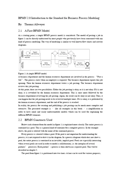
BPMN 2.0 Introduction to the Standard for Business Process Modeling By Thomas Allweyer2.1 A First BPMN ModelAs a starting point, a simple BPMN process model is considered. The model of posting a job in figure 1 can be directly understood by most people who previously have been concerned with any kind of process modeling. The way of modeling is similar to well known flow charts and activity diagrams.Figure 1: A simple BPMN modelA business department and the human resources department are involved in the process “Post a Job”. The process starts when an employee is required. The business department reports this job opening. Then the human resources department writes a job posting. The business department reviews this job posting.At this point, there are two possibilities: Either the job posting is okay, or it is not okay. If it is not okay, it is reworked by the human resources department. This is once more followed by the business department reviewing the job posting. Again, the result can be okay or not okay. Thus, it can happen that the job posting needs to be reviewed multiple times. If it is okay, it is published by the human resources department, and the end of the process is reached.In reality, the process for creating and publishing a job posting can be much more complex and extensive. The presented example is –like all examples in this book –a simplification in order to have small and easily understandable models which can be used for explaining the different BPMN elements.2.2 BPMN Constructs UsedBelow each element from the model in figure 1 is explained more closely. The entire process is contained in a pool. This is a general kind of container for a complete process. In the example above, the pool is labeled with the name of the contained process.Every process is situated within a pool. If the pool is not important for understanding the process, it is not required to draw it in the diagram. In a process diagram which does not show a pool, the entire process is contained in an invisible, implicit pool. Pools are especially interesting when several pools are used in order to model a collaboration, i.e. the interplay of several partners’processes. Each partner’s process is then shown in a separate pool. This will be described in chapter 5.The pool from figure 1 is partitioned into two lanes. A lane can be used for various purposes,e.g. for assigning organizational units, as in the example, or for representing different components within a technical system. In the example, the lanes show witch of the process’s activities are performed by the business department and which by the human resource department.Pools and lanes are also called “swimlanes”. They resemble the partitioning of swimming pools into lanes. Every participant of a competition swims only in his own lane.The process itself begins with the start event “Employee required”. Processes usually have such a start event. Its symbol is a simple circle. In most cases it makes sense to use only one start event, not several ones.A rounded rectangle represents an activity. In an activity something gets done. This is expressed by the activities’names, such as “Report Job Opening”or “Review Job Posting”.The connecting arrows are used for modeling the sequence flow. They represent the sequence in which the different events, activities, and further elements are traversed. Often this is called control flow, but in BPMN there is a second type of flow, the message flow, which influences the control of a process as well, and is therefore some kind of control flow, too. For that reason, the term “sequence flow”is used. For distinguishing it from other kinds of flow, it is important to draw sequence flows with solid lines and filled arrowheads.The process “Post a Job”contains a split: The activity “Review job posting”is followed by a gateway. A blank diamond shape stands for an exclusive gateway. This means that out of several outgoing sequence flows, exactly one must be selected. Every time the right gateway in the job posting-process is reached, a decision must be taken. Either the sequence flow to the right is followed, leading to the activity “Publish Job Posting”, or the one to the left is selected, triggering the activity “Rework Job Posting”. It is not possible to follow both paths simultaneously.The logic of such a decision is also called “exclusive OR”, abbreviated “XOR”. The conditions on the outgoing paths determine which path is selected. If a modeling tool is used and the process has to be executed or simulated by a software program, then it is usually possible to formally define exact conditions. Such formal descriptions, which may be expressed in a programming language, can be stored in special attributes of the sequence flows.If, on the other hand, the purpose of a model is to explain a process to other people,then it is advisable to write informal, but understandable, statements directly into the diagram, next to the sequence flows. The meaning of “okay”and “not okay”after the activity called “Review Job Posting”is clear to humans –a program could not make use of it.Gateways are also used for merging alternative paths. In the sample process, the gateway on the left of the activity “Review Job Posting”merges the two incoming sequence flows. Again, this is an exclusive gateway. It expects that either the activity“Write Job Posting”or “Rework Job Posting”is carried out before the gateway is reached –but not both at the same time. It should be taken care to use a gateway either for splitting or for joining, but not for a combination of both. The last element in the example process is the end event. Like the start event it has a circle as symbol –but with a thick border.2.3 Sequence Flow LogicThe flow logic of the job posting process above is rather easy to understand. In more complex models it is sometimes not clear how the modeled structure exactly is to be interpreted. Therefore it is helpful if the meaning of the sequence flow’s elements is defined in an unambiguous way.The logic of a process diagram’s sequence flow can be explained by “tokens”. Just as in a board game tokens are moved over the board according to the game’s rules, one can imagine moving tokens through a process model according to BPMN’s rules.Every time the process is started, the start event creates a token (cf. figure 2). Since the job posting process is carried out more than once, many tokens can be created in the course of time. Thereby it can happen that the process for one job posting is not yet finished, when the process for posting another job starts. As it moves through the process, each token is independent from the other tokens’movements.Figure 2: A start event creates a tokenThe token that has been created by the start event moves through the sequence flow to the first activity. This activity receives a token, performs its task (in this case it reports a job opening), and then releases it to the outgoing sequence flow (cf. figure 3).Figure 3: An activity receives a token and forwards it after completionThe following activity forwards the token. It then arrives at the merging exclusive gateway. The task of this gateway is simple: It just takes a token that arrives via any incoming sequence flow and moves it to the outgoing sequence flow. This is shown in figure 4. In case A, a token arrives from the left, in case B from below. In both cases the token is routed to the outgoing sequence flow to the right.Figure 4: Routing of a token by a merging exclusive gatewayThe task of the splitting exclusive gateway is more interesting. It takes one arriving token and decides according to the conditions, to which sequence flow it should be moved. In case A in figure 5, the condition “okay”is true, i.e. the preceding review activity has produced a positive result. In this case, the token is moved to the right. Otherwise, if the condition “not okay”is true, the token is moved to the downwards sequence flow (case B).The modeler must define the conditions in such a way that always exactly one of the conditions is true. The BPMN specification does not state how to define conditions and how to check whichconditions are true. Since the considered process is not executed by software, the rather simple statements used here are sufficient. Otherwise, it would be necessary to define the conditions according to the requirements and rules of the software tool.The token may travel several times through the loop for reworking the job posting. Finally it arrives at the end event. This simply removes any arriving token and thus finishes the entire process (figure 6).Figure 5: Routing of a token by a splitting exclusive gatewayThe sequence flow of every process diagram can be simulated in this way with the help of tokens. This allows for analyzing whether the flow logic of a process has been modeled correctly.It should be noted that a token does not represent such a thing as a data object or a document. In the case of the job posting process, it could be imagined to have a document “job posting”flowing through the process. This document could contain all required data, such as the result of the activity “Review Job Posting”. At the splitting gateway, the decision could then be based on this attribute value. However, the BPMN sequence flow is constrained to the pure order of execution. The tokens therefore do not carry any information, other than a unique identifier for distinguishing the tokens from each other. For data objects there are separate BPMN constructs which will be presented in chapter 10.2.4 Presentation OptionsUsually pools are drawn horizontally. The preferred direction of sequence flow is then from left to right. On the other hand, it is also possible to use vertical pools and to draw the sequence flow from top to bottom, as in the example in figure 7.It makes sense to decide for only one of these possibilities –horizontal or vertical. Nevertheless there are modeling tools which only support horizontal modelingFigure 6: An end event removes an arriving tokenFigure 7: Vertical swimlanes and nested lanesFigure 7 also shows an example of nested lanes. The lane labeled “Sales”is partitioned into the two lanes “Sales Force”and “Order Processing”. In principle it is possible to partition these lanes again, etc., although this only makes sense up to a certain level of depth.It is not prescribed where to place the names of pools and lanes. Typical are the variants selected for figure 1 and figure 7. Here the names are placed on the left of the pools or lanes, or at the top for the vertical style, respectively. The name of a pool is separated by a line. The names of the lanes, however, are placed directly within the lanes. A separation line is only used for a lane that is partitioned into further sub-lanes. Lanes can also be arranged as a matrix. The procurement process in figure 8 runs through a business department and the procurement department, both of which span a branch office and the headquarters. When a demand occurs in a branch’s business department, this department reports the demand. In the next step, the procurement is approved by the same department in the headquarters. The central part of the procurement department then closes a contract with a supplier, followed by the branch’s purchasing department carrying out the purchase locally.Although the BPMN specification explicitly describes the possibility of such a matrix presentation, it is hardly ever applied, so far.12.2 Message CorrelationThe contents of the message flows within one conversation are always related to each other. For example, all messages that are exchanged within one instance of the conversation “Process Order for Advertisement”relate to the same advertisement order. It is therefore possible to use the order ID for the correlation, i.e. the assignment of messages to a process instance. If a customer receives an advertisement for approval, he can determine the corresponding order –and thus the process instance –based on the order ID. All messages of a conversation have a common correlation.A simple conversation which is not broken down into other conversations is called communication. Therefore, the lines are called communication links (the specification draft at some places alsocalls them conversation links). A conversation has always communication links to two or more participants.If the end of a communication link is forked, multiple partners of the same type can be part of the communication, otherwise exactly one. “Process Order for Advertisement”has exactly one customer and one advertising agency as participants, but multiple designers. Therefore, the designer’s pool contains a multiple marker. However, having only the multiple marker in the pool is not sufficient. The conversation “Handle order for an illustration”, for example, has only one designer as participant. Therefore, the respective end of the communication link is not forked.12.3 Hierarchies of ConversationsBesides communications, it is also possible to use sub-conversations. Similar to sub-processes they are marked with a ‘+’-sign. The details of a sub-conversation can be described in another conversation diagram. The diagram of a sub-conversation can only contain those participants who are linked to the sub-conversation within the parent diagram.Figure 171 shows the detailed conversation diagram for the sub-conversation “Process Order for Advertisement”As can be seen from this diagram, it is also possible to draw message flows directly into the conversation diagram. Other than collaboration diagrams, conversation diagrams are not allowed to show processes in the pools or choreographies between the pools.Figure 171: Conversation diagram for sub-conversation “Process Order for Advertisement”The diagram contains those message flows that are related to the same order. To be more precise, they relate to the same inquiry. At the beginning, an order has not been placed yet, and not every inquiry turns into an order. Therefore, the common reference point is the inquiry.Besides the explicitly displayed message flows between customer and advertising agency, the diagram also contains the communication “Assignment of Graphics Design”. All message flows of this communication are also related to the same inquiry, but this information is not sufficient for the advertising agency in order to assign all incoming messages correctly. This is due to the fact that availability requests are sent to several designers. The advertising agency has to correctly assign each incoming availability notice to the correct availability request. Thus, additional information is required for correlating these messages, e.g. the IDs of the availability requests.Therefore it is possible to define a separate communication for the message flows between advertising agency and designer. The message exchanges of this communication can also be modeled in a collaboration diagram (figure 172) or in a choreography diagram (figure 173). Of course, it is also possible to show the message flows of the entire sub-conversation within a single diagram (figures 161 and 162 in the previous chapter).Figure 172: Collaboration diagram for communication “Assignment of Graphics Design”Like sub-processes, sub-conversations can also be expanded, i.e. the hexagon is enlarged, and the detailed conversation is shown in its interior. However, it is graphically not easy to include, for example, the contents of figure 171 into an expanded sub-conversation in figure 170. Unfortunately, the BPMN specification draft does not contain any examples for expandedsub-conversations either.。

附录英文原文：Chinese Journal of ElectronicsVo1.15,No.3,July 2006A Speaker--Independent Continuous SpeechRecognition System Using Biomimetic Pattern RecognitionWANG Shoujue and QIN Hong(Laboratory of Artificial Neural Networks，Institute ol Semiconductors，Chinese Academy Sciences，Beijing 100083，China)Abstract—In speaker-independent speech recognition,the disadvantage of the most diffused technology(HMMs，or Hidden Markov models)is not only the need of many more training samples，but also long train time requirement. This Paper describes the use of Biomimetic pattern recognition(BPR)in recognizing some mandarin continuous speech in a speaker-independent Manner. A speech database was developed for the course of study．The vocabulary of the database consists of 15 Chinese dish’s names, the length of each name is 4 Chinese words．Neural networks(NNs)based on Multi-weight neuron(MWN) model are used to train and recognize the speech sounds．The number of MWN was investigated to achieve the optimal performance of the NNs-based BPR.This system, which is based on BPR and can carry out real time recognition reaches a recognition rate of 98.14％for the first option and 99.81％for the first two options to the Persons from different provinces of China speaking common Chinese speech．Experiments were also carried on to evaluate Continuous density hidden Markov models(CDHMM ),Dynamic time warping(DTW)and BPR for speech recognition．The Experiment results show that BPR outperforms CDHMM and DTW especially in the cases of samples of a finite size．Key words—Biomimetic pattern recognition, Speech recogniton,Hidden Markov models(HMMs),Dynamic time warping(DTW)．I．IntroductionThe main goal of Automatic speech recognition(ASR)is to produce a system which will recognize accurately normal human speech from any speaker．The recognition system may be classified as speaker-dependent or speaker-independent．The speaker dependence requires that the system be personally trained with the speech of the person that will be involved with its operation in order to achieve a high recognition rate．For applications on the public facilities，on the other hand，the system must be capable of recognizing the speech uttered by many different people，with different gender，age，accent,etc.,the speaker independence has many more applications，primarily in the general area of public facilities．The most diffused technology in speaker-independent speech recognition is Hidden Markov Models，the disadvantage of it is not only the need of many more training samples，but also long train time requirement．Since Biomimetic pattern recognition(BPR) was first proposed by Wang Shoujue，it has already been applied to object recognition, face identification and face recognition etc.,and achieved much better performance．With some adaptations，such modeling techniques could be easily used within speech recognition too．In this paper，a real-time mandarin speech recognition system based on BPR is proposed，which outperforms HMMs especially in the cases of samples of a finite size．The system is a small vocabulary speaker independent continuous speech recognition one. The whole system is implemented on the PC under windows98／2000／XPenvironment with CASSANN-II neurocomputer.It supports standard 16-bit sound card ．II ．Introduction of Biomimetic Pattern Recognition and Multi —Weights Neuron Networks1． Biomimetic pattern recognitionTraditional Pattern Recognition aims at getting the optimal classification of different classes of sample in the feature space ．However, the BPR intends to find the optimal coverage of the samples of the same type. It is from the Principle of Homology —Continuity ，that is to say ，if there are two samples of the same class, the difference between them must be gradually changed ． So a gradual change sequence must be exists between the two samples. In BPR theory ．the construction of the sample subspace of each type of samples depends only on the type itself ．More detailedly ，the construction of the subspace of a certain type of samples depends on analyzing the relations between the trained types of samples and utilizing the methods of “cov erage of objects with complicated geometrical forms in the multidimensional space”.2．Multi-weights neuron and multi-weights neuron networksA Multi-weights neuron can be described as follows ：12m Y=f[(,,,)]W W W X θΦ-…，,Where ：12m ,,W W W …， are m-weights vectors ；X is the inputvector ；Φis the neuron’s computation function ；θis the threshold ；f is the activation function ．According to dimension theory, in the feature spacen R ，n X R ∈，the function12m (,,,)W W W X Φ…，=θconstruct a (n-1)-dimensional hypersurface in n-dimensional space which isdetermined by the weights12m ,,W W W …，.It divides the n-dimensional space into two parts ．If12m (,,,)W W W X θΦ=…， is a closed hypersurface, it constructs a finite subspace ．According to the principle of BPR,determination the subspace of a certain type of samples basing on the type of samples itself ．If we can find out a set of multi-weights neurons(Multi-weights neuron networks) that covering all the training samples ，the subspace of the neural networks represents the sample subspace. When an unknown sample is in the subspace, it can be determined to be the same type of the training samples ．Moreover ，if a new type of samples added, it is not necessary to retrain anyone of the trained types of samples ．The training of a certain type of samples has nothing to do with the other ones ．III ．System DescriptionThe Speech recognition system is divided into two main blocks. The first one is the signal pre-processing and speech feature extraction block ．The other one is the Multi-weights neuron networks, which performs the task of BPR ．1．Speech feature extractionMel based Campestral Coefficients(MFCC) is used as speech features ．It is calculated as follows ：A ／D conversion ；Endpoint detection using short time energy and Zero crossing rate(ZCR)；Preemphasis and hamming windowing ；Fast Fourier transform ；DCT transform ．The number of features extracted for each frame is 16，and 32 frames are chosen for every utterance ．A 512-dimensiona1-Me1-Cepstral feature vector(1632⨯ numerical values) represented the pronunciation of every word ． 2． Multi-weights neuron networks architectureAs a new general purpose theoretical model of pattern Recognition, here BPR is realized by multi-weights neuron Networks. In training of a certain class of samples ，an multi-weights neuron subNetwork should beestablished ．The subNetwork consists of one input layer ．one multi-weights neuron hidden layer and one output layer. Such a subNetwork can be considered as a mapping 512:F R R →.12m ()min(,,Y )F X Y Y =…，，Where Y i is the output of a Multi-weights neuron. There are m hiddenMulti-weights neurons ．i= 1,2, …,m,512X R ∈is the input vector ．IV ．Training for MWN Networks1． Basics of MWN networks trainingTraining one multi-weights neuron subNetwork requires calculating the multi-weights neuron layer weights ．The multi-weights neuron and the training algorithm used was that of Ref.[4]．In this algorithm ，if the number of training samples of each class is N,we can use2N -neurons ．In this paper ，N=30．12[(,,,)]ii i i Y f s s s x ++=，is a function with multi-vector input ，one scalar quantity output ．2． Optimization methodAccording to the comments in IV.1,if there are many training samples, the neuron number will be very large thus reduce the recognition speed ．In the case of learning several classes of samples, knowledge of the class membership of training samples is available. We use this information in a supervised training algorithm to reduce the network scales ．When training class A ，we looked the left training samples of the other 14 classes as class B ． So there are 30 training samples in set1230:{,,}A A a a a =…，and 420 training samples inset 12420:{,,}B B b b =…，b ．Firstly select 3 samples from A, and we have a neuron ：1123Y =f[(,,,)]k k k a a a x .Let 01_123,=f[(,,,)]A i k k k i A A Y a a a a =，where i= 1,2, (30)1_123Y =f[(,,,)]B j k k k j a a a b ，where j= 1,2,…420；1_min(Y )B j V =,we specify a value r ,0<r<1.If1_*A i Y r V <,removed i a from set A, thus we get a new set (1)A .We continue until the number ofsamples in set ()k Ais(){}k A φ=,then the training is ended, and the subNetwork of class A has a hiddenlayer of1r - neurons.V ．Experiment ResultsA speech database consisting of 15 Chinese dish’s names was developed for the course of study. The length of each name is 4 Chinese words, that is to say, each sample of speech is a continuous string of 4 words, such as “yu xiang rou si”，“gong bao ji ding”，etc ．It was organized into two sets ：training set and test set. The speech signal is sampled at 16kHz and 16-bit resolution ．Table 1．Experimental result atof different values450 utterances constitute the training set used to train the multi-weights neuron networks. The 450 ones belong to 10 speakers(5 males and 5 females) who are from different Chinese provinces. Each of the speakers uttered each of the word 3 times. The test set had a total of 539 utterances which involved another 4 speakers who uttered the 15 words arbitrarily ．The tests made to evaluate the recognition system were carried out on differentr from 0.5 to 0.95 with astep increment of 0.05.The experiment results at r of different values are shown in Table 1．Obviously ，the networks was able to achieve full recognition of training set at any r ．From the experiments ，it was found that0.5r achieved hardly the same recognition rate as the Basic algorithm. In the mean time, theMWNs used in the networks are much less than of the Basic algorithm. Table 2．Experiment results of BPR basic algorithmExperiments were also carried on to evaluate Continuous density hidden Markov models (CDHMM),Dynamic time warping(DTW) and Biomimetic pattern recognition(BPR) for speech recognition, emphasizing the performance of each method across decreasing amounts of training samples as wellas requirement of train time. The CDHMM system was implemented with 5 states per word.Viterbi-algorithm and Baum-Welch re-estimation are used for training and recognition ．The reference templates for DTW system are the training samples themselves. Both the CDHMM and DTW technique are implemented using the programs in Ref.[11]．We give in Table 2 the experiment results comparison of BPR Basic algorithm ，Dynamic time warping (DTW)and Hidden Markov models (HMMs) method ．The HMMs system was based on Continuous density hidden Markov models(CDHMMs),and was implemented with 5 states per name.VI．Conclusions and AcknowledgmentsIn this paper, A mandarin continuous speech recognition system based on BPR is established.Besides,a training samples selection method is also used to reduce the networks scales. As a new general purpose theoretical model of pattern Recognition，BPR could be used in speech recognition too, and the experiment results show that it achieved a higher performance than HMM s and DTW.References[1]WangShou-jue,“Blomimetic (Topological) pattern recognit ion-A new model of pattern recognition theoryand its application”，Acta Electronics Sinica,(inChinese)，Vo1.30,No.10,PP.1417-1420,2002．[2]WangShoujue，ChenXu，“Blomimetic (Topological) pattern recognition-A new model of patternrecognition theory and its app lication”, Neural Networks,2003.Proceedings of the International Joint Conference on Neural Networks,Vol.3,PP.2258-2262,July 20-24,2003．[3]WangShoujue,ZhaoXingtao,“Biomimetic pattern recognition theory and its applications”，Chinese Journalof Electronics，V0l.13，No.3，pp.373-377,2004．[4]Xu Jian．LiWeijun et a1,“Architecture research and hardware implementation on simplified neuralcomputing system for face identification”，Neuarf Networks，2003．Proceedings of the Intern atonal Joint Conference on Neural Networks，Vol.2,PP.948-952,July 20-24 2003．[5]Wang Zhihai,Mo Huayi et al,“A method of biomimetic pattern recognition for face recognition”,Neural Networks,2003.Proceedings of the International Joint Conference on Neural Networks,Vol.3，pp.2216-2221,20-24 July 2003．[6]WangShoujue,WangLiyan et a1,“A General Purpose Neuron Processor with Digital-Analog Processing”，Chinese Journal of Electornics,Vol.3,No.4,pp.73-75,1994．[7]Wang Shoujue,LiZhaozhou et a1,“Discussion on the basic mathematical models of neurons in gen eralpurpose neuro-computer”，Acta Electronics Sinica(in Chinese),Vo1.29,No.5,pp.577-580,2001．[8]WangShoujue,Wang Bainan,“Analysis and theory of high-dimension space geometry of artificial neuralnetworks”,Acta Electronics Sinica (in Chinese)，Vo1.30，No.1,pp.1-4,2001．[9]WangShoujue,Xujian et a1,“Multi-camera human-face personal identiifcation system based on thebiomimetic pattern recognition”，Acta Electronics Sinica (in Chinese)，Vo1.31,No.1,pp.1-3,2003．[10]Ryszard Engelking,Dimension Theory,PWN-Polish Scientiifc Publishers—Warszawa,1978．[11]QiangHe,YingHe,Matlab Porgramming,Tsinghua University Press，2002．中文翻译：电子学报2006年7月15卷第3期基于仿生模式识别的非特定人连续语音识别系统王守觉秦虹（中国，北京100083，中科院半导体研究所人工神经网络实验室）摘要：在非特定人语音识别中，隐马尔科夫模型（HMMs）是使用最多的技术，但是它的不足之处在于：不仅需要更多的训练样本，而且训练的时间也很长。

1.Today my friend and I are taking a walk。

suddenly，we are seeing a boy sit on the chair,he is crying，we go and ask him。

“what’s the matter with you” he tell us“I can’t find my dog can you help me”.“yes,I can”.And we help him find his dong .oh it stay underthe big tree!今天我和我的朋友一起去散步。

突然我们看见一个男孩坐在椅子上，他哭的很伤心。

我们走过去问他：“你怎么了”。

他告诉我们：“我的狗不见了，你们能帮我找到它吗”.“是的，我们能帮你找到你的狗”然后我们帮助他找到了他的狗，原来是它呆在一棵大树下。

2。

One day an old man siselling a big elephant.A young man comes to the elephant and begins to look at it slowly。

The old man goes up to him and says inhis ear，“Don't say anything about the elephant before I sell it，then i'll give you some money."“All right，”says the young man.After the old man slles the elephant，he gives the young man some money and says，“Now,can you tell me how you find the bad ears of theelephant？”“I don’t find the bad ears，”says the young man.“Then why do you look at the elephant slowly?”asks the old man。

名篇名译0011.原文：It is an ill wind that blows nobody good.译文：世事皆利弊并存。

赏析：原句结构比较特殊（"It is … that …"），理解起来有点困难。

“对谁都没有好处的风才是坏风”，也就是说大多数情况下风对人都是有好处、有坏处，在引申一步就是成了上面的译句。

林佩耵在《中英对译技巧》一书中（第68页）还给了几个相同结构的英文句子。

翻译的前提是理解。

有人指出。

市面上见到的翻译作品，有好多都带有因理解不正确而产生的低级错误，“信”都谈不上还妄谈什么“达”和“雅”！初学翻译的朋友，在理解原文上当不遗余力。

2.原文：Their language was almost unrestrained by any motive of prudence.译文：他们几乎爱讲什么就讲什么，全然不考虑什么谨慎不谨慎。

赏析：如果硬译，译文势必成了“他们的言论几乎不受任何深思熟虑的动机的约束”。

译者本其译，化其滞，将原句一拆为二，充分运用相关翻译技巧，译文忠实、通顺。

3.原文：Get a livelihood,and then practise virtue.译文：先谋生而后修身。

（钱钟书译）赏析：原句是祈使句，译句也传达出了训导的意味。

用“谋生”来译“Get a livelihood"，用“修身”来译“practise virtue",可谓精当。

巧的是，原句七个词，译句也是七个汉字。

4.原文：I enjoy the clean voluptuousness of the warm breeze on my skin and the cool support of water.译文：我喜爱那洁净的暖风吹拂在我的皮肤上使我陶然欲醉，也喜爱那清亮的流水把我的身体托浮在水面。

（章振邦译）赏析："voluptuousness"不会"clean",是"breeze""clean","support"不会"cool", 是"water""cool"，这种“甲乙两项相关联，就把原属于形容甲的修饰语移属于乙”的修饰手法叫“移就”（transferred epithet）（《英语修辞赏析》，第145页）。

英文资料翻译原文Boiler management:General management principles and operating procedures are well known and must be always followed to avoid boiler mishap.With many small package boiler,the automatic control sequence usually ensures that the boiler fire is initially ignited from a diesel oil supply,and changed over to the usual source when ignition is completed.With good management ,to facilitate subsequent starting from cold,the fuel system of large boilers will have been flushed through with diesel oil when the boiler was on light duty immediately prior to being secured.When burning such diesel fuel it is essential for safety that only the correct(small) burner tip should be used.It should be kept in mind that if fire does not light,immediately shut off fuel and vent furance.Complete ignition of fuel in the furance is essential.The burner flame,the smoke indicator and the funnel should be frequently observed.With satisfactory combustion,the flame should appear incandescent with an orange shade at the flame tip,and a faint brownish haze should show at the funnel.If on fist ignition the flame is uncertain,badly shaped and separates from the primary swirler ,momentary opening or closing of air register may correct.The PH value of the boiler feed water should kept between 8 and 9 and the boiler density less than 300 ppm but,if water samples show a heavy concentration of suspended mater,short blow-downs of 20 seconds duration should be given until the sludge content is seen to be reduced.The boiler should be blown down when the oil burner is operating,the water level lowered and then restored to prove the functioning of the low water cut-out and the oil burner start-up equipment.the boiler scum valve should also be operated at this time to keep the water level clear floating scum.Fuel burner components and igniter electrodes should be cleaned weekly and the furance examined to ensure that there are no excess carbon deposits.Tubes in the exhaust gas section of the boiler should be brushed through at about six-monthly intervals,and those in the oil-burning section periodically examined and cleaned as necessary with a wire bristle brush.With correct feed water treatment,blow-down procedures and sludge contents in water samples at a stable level,it should not be necessary to wash out the water side of the boiler more than once every three or four months.Boiler fires may be out of for long periods when a ship is at sea and the boiler steaming maintained by heat input from waste heat recovery plant.This operation is free from hazard,but feed water and boiler water treatment must be maintained to prevent internal deterioration or scale formation.Water level controller must be kept operable to protect external steam-using plant from water “carry-over”danger.If a boiler is isolated from the steam-using system it must be kept either in closed dry storage with a suitable internal desiccant,or completely full of treated water,or under a low steam pressure preferably maintained by a steam-heated coil.Regular testing of boiler protective devices must be implemented.Frequent comparison of drum-mounted and remote reading water levelindicators:discrepancies between these have contributed to failures because of overheating through shortage of water,when a boiler was being oil-fired.If in doubt as to the true boiler water level,i.e.whether a water level indicator sightglass is completely full or empty,when a unit is being oil-fired the fire should be immediately extinguished until the true level is resolved.Procedures should be predetermined and followed in the event of shortage of water,bulging or fracture of plates or furance,or bursting of water tubes .In general,fires should be immediately extinguished by remote tripping of fuel supply valves;forced draught air pressure maintained if there is any risk of escaping steam entering the boiler room;stem pressure relieved if metallic fractures seem possible;and boiler water level maintained,where practicable,until the boiler begins to cool down. Regular operation of soot blowers,if there are fitted,when the boiler is on oil-fired operation.The steam supply line must be thoroughly warmed and drained before blowers are used,the air/fuel ratio increased throughout the action,and the blowers greased after use.Immediate investigation of any high salinity alarms in condensate system,and elimination of any salt water or oil contamination of boiler feed water system. Safety precautions taken before entering a boiler connected to another boiler under steam.Engine governor:A governor maintains the engine speed at the desired value no matter how much load is applied.It achieves this by adjustment of the fuel pump racks.Any change in load will produce a change in engine speed,which will cause the governor to initiate a fuel change.The governor is said to be speed sensing as a speed change has to take place before the governor can react to adjust the fuel setting.The sample mechanical governor employs rotating weights which move outward as the speed increases and inward as the speed reduces.This movement,acting through a system of linkages,can be used to regulate the fuel rack.Rather than having the rotating weights directly move the fuel linkage,hydraulic governor employ a servo system so the rotating weights only need to move a pilot valve in the hydraulic line.This makes the governor more ernors of this type require a speed change to tale place in order that they may initiate fuel rack adjustment.This is known as speed drop and this is a definite speed for each load therefore the governor can not control to a single speed.A modification to the governor hydraulic system introduces a facility known as compensation which allows for further fuel adjustment after the main adjustment has taken place due to speed pensation restores the speed to its original desired value so the engine can operate at the same speed under all loads.Such a governor is said to be isochronous as the engine operates at a single speed.However,the governor is still speed sensing,so it is not ideal for all applications.Speed sensing governor:Where the engine drives an alternator any speed change results in a change in supply frequency.;Large changes in electrical supply frequency can have an adverse effect on sensitive electronic equipment connected to that supply.Where electrical generation is involved it is possible to monitor taking rotational speed as the control signal.Such governors are know as load sensing.It isextremely difficult to make a mechanical governor load sensing,even with a hydraulic system,but an electronic governor can take account of the electrical load applied to the engine and so can be considered “speed sensing”.Electronic governor:Electronic governors essentially comprise two parts,the digital control unit and the hydraulic actuator,which are interlinked but it is useful to consider them separately.Electronic governor controller: The digital control may be considered as a “black box” in which signals are processed to produce a control signal which is sent to the actuator.The controller may be programmed in order to sent points and parameters.The controller is a sensitive piece of electronic equipment and should not be mounted on the engine or in areas where it will be exposed to vibration,humidity or high temperatures.It should be ventilated in order to keep it cool and should be shielded from high-voltage or high-current devices which will cause electromagnetic interference.Similar restriction apply to the location of signal cables.Speed signals are taken from two speed transducers,one on each side of the flexible coupling which attaches the engine to the load.Failure of one transducer produces a minor alarm but allows continued operation with an electronic over speed value may be programmed into the controller in which case detection of over speed will cause the engine to be shut off.If the load is provided by an electrical machine the output from that machine provides a signal for load sharing.Should this transducer fail the load on the engine will be determined by the position of the governor actuator output.The controller can also receive signals from other transducers including in the engine’s air inlet pressure,which allows the fuel to be limited when starting.After processing input signals in accordance with programmed requirements an output signal will be sent to the governor actuator.Electronic governor actuator:The actuator is a hydraulic device which moves the fuel linkage in response to a signal from the digital controller.The operating mechanism is contained with an oil filled casing.Oil pressure is provided by a servomotor pump driven by a shaft connected to the engine camshaft.At the heart of the actuator is the torque motor beam is banlanced where the engine is operating at the desired speed.a.Consider a load increaseThe controller increases current to the torque motor which,in turn,causes the centre adjust end of the torque motor beam to be lowered.Oil flow through the nozzle is reduced ,which increases pressure on the top of the pilot valve plunger.This moves downward,unconering the port which allows pressure oil to the lower face of the power piston,which in turn moves upward, rotating the terminal shaft thereby increasing the fuel to the engine.As the terminal shaft rotates the torque motor beam is pulled upwards by increased tension in the feedback spring,increasing the clearance between the centers adjust and the nozzle.Leakage past the nozzle increases,reducing the pressure on the upper face of the pilot valve plunger and allowing the pilot valve to move upwards.This cuts off further oil to the power piston,and movement of the fuel control linkage ceases.Balance is restored to the torque motor beam with downward force from the feedback spring being matched by upwards force from oilleakage from the nozzle.The engine then operates at an increased fuel setting which matches the new load requirement at the set speed.B.consider a load reductionA decrease in load produces a reduction in current acting on the torque motor,which tends to turn the beam in an anti-clockwise direction about the torque motor pivot,resulting in an increased clearance between the centre adjust and the nozzle.Pressure reduces on the upper face of the pilot valve plunger and the pilot valve moves upwards,allowing the lower face of the power piston to connect with the geromotor pump suction.the power piston moves downwards ,rotating the terminal shaft which reduces fuel to the engine and tension in the feedback spring.The center adjust end of the torque motor beam is forced down,thereby reducing clearance between the centre adjust and the nozzle.Leakage past the nozzle reduces pressure on the upper face of the pilot valve increases and the pilot valve moves upwards,shuting off the connection between the lower face of the power piston and pump suction .The engine now operates with reduced load and reduced fuel,but at the same original speed.。

英文原文：Rehabilitation of rectangular simply supported RC beams with shear deficienciesusing CFRP compositesAhmed Khalifa a,* , Antonio Nanni ba Department of Structural Engineering, University of Alexandria, Alexandria 21544, Egyptb Department of Civil Engineering, University of Missouri at Rolla, Rolla, MO 65409, USAReceived 28 April 1999; received in revised form 30 October 2001; accepted 10 January 2002AbstractThe present study examines the shear performance and modes of failure of rectangular simply supported reinforced concrete(RC) beams designed with shear deficiencies. These members were strengthened with externally bonded carbon fiber reinforced polymer (CFRP) sheets and evaluated in the laboratory. The experimental program consisted of twelve full-scale RC beams tested to fail in shear. The variables investigated within this program included steel stirrups, and the shear span-to-effective depth ratio, as well as amount and distribution of CFRP. The experimental results indicated that the contribution of externally bonded CFRP to the shear capacity was significant. The shear capacity was also shown to be dependent upon the variables investigated. Test results were used to validate a shear design approach, which showed conservative and acceptable predictions.○C2002 Elsevier Science Ltd. All rights reserved.Keywords: Rehabilitation; Shear; Carbon fiber reinforced polymer1. IntroductionFiber reinforced polymer (FRP) composite systems, composed of fibers embedded in a polymeric matrix, can be used for shear strengthening of reinforced con-crete (RC) members [1–7]. Many existing RC beams are deficient and in need of strengthening. The shear failure of an RC beam is clearly different from its flexural failure. In shear, the beam fails suddenly without sufficient warning and diagonal shear cracks are consid-erably wider than the flexural cracks [8].The objectives of this program were to:1. Investigate performance and mode of failure of simply supported rectangular RC beams with shear deficien-cies after strengthening with externally bonded CFRP sheets.2. Address the factors that influence shear capacity of strengthened beams such as: steel stirrups, shear span-to-effective depth ratio (a/d ratio), and amount and distribution of CFRP.3. Increase the experimental database on shear strength-ening with externally bonded FRP reinforcement.4. Validate the design approach previously proposed by the authors [9].For these objectives, 12 full-scale, RC beams designed to fail in shear were strengthened with different CFRP schemes. These members were tested as simple beams using a four-point loading configuration with two different a/d ratios.2. Experimental program2.1. Test specimens and materialsTwelve full-scale beam specimens with a total span of 3050 mm. and a rectangular cross-section of 150-mm-wide and 305-mm-deep were tested. The specimens were grouped into two main series designated SW and SO depending on the presence of steel stirrups in the shear span of interest.Series SW consisted of four specimens. The details and dimensions of the specimens designated series SW are illustrated in Fig. 1a. In this series, four 32-mm steel bars were used as longitudinal reinforcement with two at top and two at bottom face of the cross-section to induce a shear failure. The specimens were reinforced with 10-mm steel stirrups throughout their entire span. The stirrups spacing in the shear span of interest, right half, was selected to allow failure in that span.Series SO consisted of eight beam specimens, which had the same cross-section dimension and longitudinal steel reinforcement as for series SW. No stirrups were provided in the test half span as illustrated in Fig. 1b.Each main series (i.e. series SW and SO) was subdivided into two subgroups according to shear span-to-effective depth ratio. This was selected to be a/d = 3 and 4, resulting in the following four subgroups: SW3;SW4; SO3; and SO4.The mechanical properties of the materials used for manufacturing the test specimens are listed in Table 1.Fabrication of the specimens including surface preparation and CFRP installation is described elsewhere [10].Table 12.2. Strengthening schemesOne specimen from each series (SW3-1, SW4-1, SO3-1 and SO4-1) was left without strengthening as a control specimen, whereas eight beam specimens were strengthened with externally bonded CFRP sheets following three different schemes as illustrated in Fig. 2.In series SW3, specimen SW3-2 was strengthened with two CFRP plies having perpendicular fiber directions (90°/0°). The first ply was attached in the form of continuous U-wrap with the fiber direction oriented perpendicular to the longitudinal axis of the specimen (90°). The second ply was bonded on the two sides of the specimen with the fiber direction parallel to the beam axis（0°）.This ply [i.e. 0°ply] was selected to investigate the impact of additional horizontal restraint on shear strength.In series SW4, specimen SW4-2 was strengthened with two CFRP plies having perpendicular fiber direction (90°/0°) as for specimen SW3-2.Four beam specimens were strengthened in series SO3. Specimen SO3-2 was strengthened with one-ply CFRP strips in the form of U-wrap with 90°-fiber orientation. The strip width was 50 mm with center-to-center spacing of 125 mm. Specimen SO3-3 was strengthened in a manner similar to that of specimen SO3-2, butwith strip width equal to 75 mm. Specimen SO3-4 was strengthened with one-ply continuous U-wrap (90°). Specimen SO3-5 was strengthened with twoCFRP plies (90°/0°) similar to specimens SW3-2 and SW4-2.In series SO4, two beam specimens were strengthened. Specimen SO4-2 was strengthened with one-ply CFRP strips in the form of U-wrap similar to specimen SO3-2. Specimen SO4-3 was strengthened with one-ply continuous U-wrap (90°) similar to SO3-4.2.3. Test set-up and instrumentationAll specimens were tested as simple span beams subjected to a four-point load as illustrated in Fig. 3. A universal testing machine with 1800 KN capacity was used in order to apply a concentrated load on a steel distribution beam used to generate the two concentrated loads. The load was applied progressively in cycles, usually one cycle before cracking followed by three cycles with the last one up to ultimate. The applied load vs. deflection curves shown in this paper are the envelopes of these load cycles.Four linear variable differential transformers (LVDTs) were used for each test to monitor vertical displacements at various locations as shown in Fig. 3. Two LVDTs were located at mid-span on each side of the specimen. The other two were located at the specimen supports to record support settlement.For each specimen of series SW, six strain gauges were attached to three stirrups to monitor the stirrup strain during loading as illustrated in Fig. 1a. Three strain gauges were attached directly to the FRP sheet on the sides of each strengthened beam to monitor strain variation in the FRP. The strain gauges were oriented in the vertical direction and located at the section mid-height with distances of 175, 300 and 425 mm, respectively, from the support for series SW3 and SO3. For beam specimens of series SW4 and SO4, the strain gauges were located at distance of 375, 500 and 625 mm, respectively, from the support.3. Results and discussionIn the following discussion, reference is always made to weak shear span or span of interest.3.1. Series SW3Shear cracks in the control specimen SW3-1 were observed close to the middle of the shear span when the load reached approximately 90 kN. As the load increased, additional shear cracks formed throughout, widening and propagating up to final failure at a load of 253 kN (see Fig. 4a).In specimen SW3-2 strengthened with CFRP (90°/0°), no cracks were visible on the sides or bottom of the test specimen due to the FRP wrapping. However，a longitudinal splitting crack initiated on the top surface of the beam at a high load of approximately 320 kN.The crack initiated at the location of applied load and extended towards the support. The specimen failed by concrete splitting (see Fig. 4b) at total load of 354 kN. This was an increase of 40% in ultimate capacity compared to the control specimen SW3-1. The splitting failure was due to the relatively high longitudinal compressive stress developed at top of the specimen, which created a transverse tension, led to the splitting failure. In addition, the relatively large amount of longitudinal steel reinforcement combined with over-strengthening for shear by CFRP wrap probably caused this mode of failure. The load vs. mid-span deflection curves for specimens SW3-1 and SW3-2 are illustrated in Fig. 5, to show the additional capacity gained by CFRP.The maximum CFRP vertical strain measured at failure in specimen SW3-2 was approximately 0.0023 mm/mm, which corresponded to 14% of the reported CFRP ultimate strain. This value is not an absolute because it greatly depends on the location of the strain gauges with respect to a crack. However, the recorded strain indicates that if the splitting did not occur, the shear capacity could have reached higher load.Comparison between measured local stirrup strains in specimens SW3-1 and SW3-2 are shown in Fig. 6. The stirrups 1, 2 and 3 were located at distance of 175, 300 and 425 mm from the support, respectively. The results showed that the stirrups 2 and 3 did not yield at ultimate for both specimens. The strains (and the forces) in the stirrups of specimen SW3-2 were, in general, smaller than those of specimen SW3-1 at the same level of loading due to the effect of CFRP.Fig. 6. Applied load vs. strain in the stirrups for specimens SW3-1 and SW3-2. 3.2. Series SW4In specimen SW4-1, the first diagonal crack was formed in the member at a totalapplied load of 75 kN. As the load increased, additional shear cracks appeared throughout the shear span. Failure of the beam occurred when the total applied load reached 200 kN. This was a decrease of 20% in shear capacity compared to the specimen SW3-1 with a/d ratio=3.In specimen SW4-2, the failure was controlled by concrete splitting similar to test specimen SW3-2. The total applied load at ultimate was 361 kN with an 80% increase in shear capacity compared to the control specimen SW4-1. In addition, the measured strains in the stirrups for specimen SW4-2 were less than those of specimen SW4-1. The applied load vs. mid-span deflection curves for beams SW4-1 and SW4-2 are illustrated in Fig. 7. It may be noted that specimen SW4-2 resulted in greater deflection when compared to specimen SW4-1.When comparing the test results of series SW3 specimens to that of series SW4, the ultimate failure load of specimen SW3-2 and SW4-2 was almost the same. However, the enhanced capacity of specimen SW3-2 (a/d=3) due to the addition of the CFRP reinforcement was 101 kN, while specimen SW4-2 (a/d=4) was 161 kN. This indicates that the contribution of external CFRP reinforcement may be influenced by the ayd ratio and appears to decrease with a decreasing a/d ratio. Further, for both strengthened specimens (SW3-2 and SW4-2), CFRP sheets did not fracture or debond from the concrete surface at ultimate and this indicates that CFRP could provide additional strength if the beams did not failed by splitting.3.3. Series SO3Fig. 8 illustrates the failure modes for series SO3 specimens. Fig. 9 details the applied load vs. mid-span deflection for the specimens.The failure mode of control specimen SO3-1 was shear compression. Failure of the specimen occurred at a total applied load of 154 kN. This load was a decrease of shear capacity by 54.5 kN compared to the specimen SW3-1 due to the absent of the steel stirrups. In addition, the crack pattern in specimen SW3-1 was different from of specimen SO3-1. In specimen SW3-1, the presence of stirrups provided a better distribution of diagonal cracks throughout the shear span.In specimen SO3-2, strengthened with 50-mm CFRP strips spaced at 125 mm, the first diagonal shear crack was observed at an applied load of 100 kN. The crackpropagated as the load increased in a similar manner to that of specimen SO3-1. Sudden failure occurred due to debonding of the CFRP strips over the diagonal shear crack, with spalled concrete attached to the CFRP strips. The total ultimate load was 262 kN with a 70% increase in shear capacity over the control specimen SO3-1. The maximum local CFRP vertical strain measured at failure in specimen SO3-2 was 0.0047 mm/mm (i.e. 28% of the ultimate strain), which indicated that the CFRP did not reach its ultimate.Specimen SO3-3, strengthened with 75-mm CFRP strips failed as a result of CFRP debonding at a total applied load of 266 kN. No significant increase in shear capacity was noted compared to specimen SO3-2. The maximum-recorded vertical CFRP strain at failure was 0.0052 mmymm (i.e. 31% of the ultimate strain).Specimen SO3-4, which was strengthened with a continuous CFRP U-wrap (908), failed as a result of CFRP debonding at an applied load of 289 kN. Results show that specimen SO3-4 exhibited increase in shear capacity of 87, 10 and 8.5% over specimens SO3-1,SO3-2 and SO3-3, respectively. Applied load vs. vertical CFRP strain for specimen SO3-4 is illustrated in Fig. 10 in which strain gauges sg1, sg2 and sg3 were located at mid-height with distances of 175, 300 and 425 mm from the support, respectively. Fig.10 shows that the CFRP strain was zero prior to diagonal crack formation, then increased slowly until the specimen reached a load in the neighborhood of the ultimate strength of the control specimen. At this point, the CFRP strain increased significantly until failure. The maximum local CFRP vertical strain measured at failure was approxi- mately 0.0045 mm/mm.When comparing the results of beams SO3-4 and SO3-2, the CFRP amount used to strengthen specimen SO3-4 was 250% of that used for specimen SO3-2. Only a 10% increase in shear capacity was achieved for the additional amount of CFRP used. This means that if an end anchor to control FRP debonding is not used, there is an optimum FRP quantity, beyond which the strengthening effect is questionable. A previous study [11] showed that by using an end anchor system, the failure mode of FRP debonding could be avoided. Reported findings are consistent with those of other research [7],which was based on a review of the experimental results available in the literature, and indicated that the contribution of FRP to the shear capacity increases almost linearly, with FRP axial rigidity expressed byf f E ρ(f ρ is the FRP area fraction and f E is the FRP elastic modulus) up to approximately 0.4 GPa. Beyond this value, the effectiveness of FRP ceases to be positive.In specimen SO3-5, the use of a horizontal ply over the continuous U-wrap (i.e. 90°/0°) resulted in a concrete splitting failure rather than a CFRP debonding failure. The failure occurred at total applied load of 339 kN with a 120% increase in the shear capacity compared to the control specimen SO3-1. The strengthening with two perpendicular plies (i.e. 90°/0°) resulted in a 17% increase in shear capacity compared to the specimen with only one CFRP ply in 90° orientation (i.e. specimen SO3-4). The maximum local CFRP vertical strain measured at failure was 0.0043 mm/mm.By comparing the test results of specimens SW3-2 and SO3-5, having the same a/d ratio and strengthening schemes but with different steel shear reinforcement, the shear strength (i.e. 177 and 169.5 kN for specimens SW3-2 and SO3-5, respectively), and the ductility are almost identical. One may conclude that the contribution of CFRP benefits the beam capacity to a greater degree for beams without steel shear reinforcement than for beams with adequate shear reinforcement.3.4. Series SO4Series SO4 exhibited the largest increase in shear capacity compared to the other series investigated with this research study. The experimental results in terms of applied load vs mid-span deflection for this series is illustrated in Fig. 11.The control specimen SO4-1 failed as a result of shear compression at a total applied load of 130 kN. Specimen SO4-2, strengthened with CFRP strips, the failure was controlled by CFRP debonding at a total load of 255 kN with 96% increase in shear capacity over the control specimen SO4-1. The maximum local CFRP vertical strain measured at failure was 0.0062mmymm.When comparing the test results of specimen SO4-2 to that of specimen SO3-2, theenhanced shear capacity of specimen SO4-2 (a/d=4) due to addition of CFRP strips was 62.5 kN, while specimen SO3-2 (a/d=3) resulted in added shear capacity of 54 kN. As expected, the contribution of CFRP reinforcement to resist the shear appeared to decrease with decreasing a/d ratio. Specimen SO4-3, strengthened with continuous U- wrap, failed as a result of concrete splitting at an applied load of 310 kN with a 138% increase in shear capacity compared to that of specimen SO4-1. The maximum local CFRP vertical strain measured at failure was 0.0037 mm/mm.4. Design approachThe design approach for computing the shear capacity of RC beams strengthened with externally bonded CFRP reinforcement, expressed in ACI design code [12] format, was proposed and published in 1998 [13]. The design model described two possible failure mechanisms of CFRP reinforcement namely: CFRP fracture; and CFRP debonding. Furthermore, two limits on the contribution of CFRP shear were proposed. The first limit was set to control the shear crack width and loss of aggregate interlock, and the second was to preclude web crushing. Also, the concrete strength and CFRP wrap- ping schemes were incorporated as design parameters. In recent study [9,10], modifications were proposed to the 1998 design approach to include results of a new study on bond mechanism between CFRP sheets and concrete surface [14]. In addition, the model was extended to provide the shear design equations in Eurocode as well as ACI format. Comparing with all test results available in the literature to date, 76 tests, the design approach showed acceptable and conservative estimates [10,13]. In this section, the summary of the design approach is presented. The comparison between experimental results and the calculated factored shear strength demonstrates the ability of the design approach to predict the shear capacity of the strengthened beams. demonstrates the ability of the design approach to predict the shear capacity of the strengthened beams.4.1. Summary of the shear design approach — ACI formatIn traditional shear design (including the ACI Code), the nominal shear strength of an RC section is the sum of the nominal shear strengths of concrete and steel shear reinforcement. For beams strengthened with externally bonded FRP reinforcement,the shear strength may be computed by the addition of a third term to account of the FRP contribution. This is expressed as follows:The design shear strength,n V φ, is obtained by multiplying the nominal shear strength by a strength reduction factor for shear,φ. It was suggested that the reduction factor φ=0.85 given in ACI [12] be main-tained for the concrete and steel terms. However, a more stringent strength reduction factor of 0.7 for the CFRP contribution was suggested w10x. This is due to the relative novelty of this repair technique. Thus, the design shear strength is expressed as follows.4.2. Contribution of CFRP reinforcement to the shear capacityThe expression used to compute shear contribution of CFRP reinforcement is given in Eq. (3). This equation is similar to that for shear contribution of steel stirrups and consistent with the ACI format.The area of CFRP shear reinforcement,f A , is the total thickness of the sheet (usually f t 2or sheets on both sides of the beam) times the width of the CFRP stripf ω. The dimensions used to define the area of CFRP in addition to the spacingf s and the effective depth of CFRP,f d ， are shown in Fig. 12. Note that for continuous verticalshear reinforcement, the spacing of the strip,f s , and the width of the strip, f ω, areequal. In Eq. (3), an effective average CFRP stressfe f , smaller than its ultimate strength,fu f , was used to replace the yield stress of steel. At the ultimate limit state for the member in shear, it is not possible to attain the full strength of the FRP [7,13]. Failure is governed by either fracture of the FRP sheet at average stress levels wellbelow FRP ultimate capacity due to stress concentrations, debonding of the FRP sheet from the concrete surface, or a significant decrease in the post- cracking concrete shear strength from a loss of aggregate interlock. Thus, the effective average CFRP stress is computed by applying a reduction coefficient, R, to the CFRP ultimate strength as expressed in Eq. (4).The reduction coefficient depends on the possible failure modes (either CFRP fracture or CFRP debonding). In either case, an upper limit for the reduction coefficient is established in order to control shear crack width and loss of aggregate interlock.4.3. Reduction coefficient based on CFRP sheet fracture failureThe proposed reduction coefficient was calibrated on all available test results to date, 22 tests with failure controlled by CFRP fracture [10，13]. The reduction coefficient was established as a function off f E ρ (where f ρis the area fraction of CFRP) and expressed in Eq.(5) for ≤f f E ρ0.7 GPa.4.4. Reduction coefficient based on CFRP debonding failureThe shear capacity governed by CFRP debonding from the concrete surface was presented [9,10]as a function of CFRP axial rigidity, concrete strength, effective depth of CFRP reinforcement, and bonded surface configurations. In determining the reduction coefficient for bond, the effective bond length, e L , has to be determined first. Based on analytical and experimental data from bond tests, Miller [14] showed that the effective bond length slightly increases as CFRP axial rigidity,f f E t , increases. However, he suggested a constant conservative value e L for equal to 75 mm. The value may be modified when more bond tests data becomes available.After a shear crack develops, only that portion of the width of CFRP extending past the crack by the effective bonded length is assumed to be capable of carrying shear.[13] The effective width,fe W , based on the shear crack angle of 45°, and thewrapping scheme is expressed in Eqs. (6a) and (6b);if the sheet in the form of a U-wrap (6a)if the sheet is bonded only to the sides of the beam. (6b)The final expression for the reduction coefficient, R, for the mode of failure controlled by CFRP debonding is expressed in Eq. (8)Eq. (7) is applicable for CFRP axial rigidity, f f E t , ranging from 20 to 90 mm-GPa (kN/mm). Research into quantifying the bond characteristics for axial rigidities above 90 mm·GPa is being conducted at the University of Missouri, Rolla (UMR).4.5. Upper limit of the reduction coefficientIn order to control the shear crack width and loss of aggregate interlock, an upper limit of reduction coefficient, R, was suggested and calibrated with all of the available test results [10] to be equal to fu ε/006.0where fu εis the ultimate tensile CFRP strain. This limit is such that the average effective strain in CFRP materials at ultimate can not be greater than 0.006 mm/mm (without the strengthening reduction factor,φ).4.6. Controlling reduction coefficientThe final controlling reduction coefficient for the CFRP system is taken as the lowest value determined from the two possible modes of failure and the upper limit. Note that if the sheet is wrapped entirely around the beam or an effective end anchor is used, the failure mode of CFRP debonding is not to be considered. The reduction coefficient is only controlled by FRP fracture and the upper limit.4.7. CFRP spacing requirementsSimilar to steel shear reinforcement, and consistent with ACI provision for the stirrups spacing [12], the spacing of FRP strips should not be so wide as to allow the formation of a diagonal crack without intercepting a strip. For this reason, if strips are used, they should not be spaced by more than the maximum given in Eq. (8).4.8. Limit on total shear reinforcementACI 318M-95 [12] 11.5.6.7 and 11.5.6.8 set a limit on the total shear strength that may be provided by more than one type of shear reinforcement to preclude the webcrushing. FRP shear reinforcement should be included in this limit. A modification to ACI 318M-95 Section 11.5.6.8 was suggested as follows:4.9. Shear capacity of a CFRP strengthened section — Eurocode formatThe proposed design equation wEq. (3)x for computing the contribution of externally bonded CFRP reinforcement may be rewritten in Eurocode (EC2 1992) [15] format as Eq. (10).In this equation, the partial safety factor for CFRP materials,f , was suggestedequal to 1.3 [10].4.10. Comparison between the test results and calculated valuesThe test summary and the comparison between the test results and the calculated shear strength, using the design approach (ACI format), are detailed in Tables 2 and 3, respectively. For CFRP strengthened beams, the measured contribution of concrete, Vc , and steel stirrups, Vs, (when present) were considered equal to the shearstrength of a non-strengthened beam. The nominal shear strength provided by concrete and steel stirrups was computed using Equations (11-5) and (11-15) in ACI- 318-95 [12]. In Equation (11-5), the values of Vu and M u were taken at the point of application of the load. The comparison indicates that the design approach gives conservative results for the strengthened beams as illus-trated in Fig. 13.5. Conclusions and further recommendationAn experimental investigation was conducted to study the shear behavior and the modes of failure of simply supported rectangular section RC beams with shear deficiencies, strengthened with CFRP sheets. The parameters investigated in this program were existence of steel shear reinforcement, shear span-to-effective depth ratio (ayd ratio), and CFRP amount and distribution.The results confirm that the strengthening technique using CFRP sheets can be used toincrease significantly shear capacity, with efficiency that varies depending on the tested variables. For the beams tested in this program, increases in shear strength of 40–138% were achieved.Conclusions that emerged from this study may be summarized as follows:●The contribution of externally CFRP reinforcement to the shear capacity isinfluenced by the a/d ratio.●Increasing the amount of CFRP may not result in a proportional increase in theshear strength. The CFRP amount used to strengthen specimen SO3-4 was 250% of that used in specimen SO3-2, which resulted in a minimal (10%) increase in shear capacity. An end anchor is recommended if FRP debonding is to be avoided. Table2Table3●The test results indicated that contribution of CFRP benefits the shear capacity at agreater degree for beams without shear reinforcement than for beams with adequate shear reinforcement.●The results of series SO3 indicated that the 0° ply improved the shear capacity byproviding horizontal restraint.●The shear design algorithms provided acceptable and conservative estimates forthe strengthened beams. Recommendations for future research are as follows:●Experimental and analytical investigations are required to link the shearcontribution of FRP with the load condition. These studies have to consider both the longitudinal steel reinforcement ratio and the concrete strength as parameters.Laboratory specimens should maintain practical dimensions.●The strengthening effectiveness of FRP has to be addressed in the cases of shortand very short shear spans in which arch action governs failure.●The interaction between the contribution of external FRP and internal steel shearreinforcement has to be investigated.●To optimize design algorithms, additional specimens need to be tested withdifferent CFRP amount and configurations to create a large database of information.●Shear design algorithms need to be expanded to include strengthening with aramid。

Journal of Molecular Catalysis A:Chemical238(2005)192–198Efficient azo dye degradation by hydrogen peroxide oxidation withmetalloporphyrins as catalystsArm´e nio C.Serra a,Cristina Docal b,A.M.d’A.Rocha Gonsalves b,∗a Universidade Cat´o lica Portuguesa-P´o lo da Figueira da Foz,Rua Dr.Mendes Pinheiro24,3080-Figueira da Foz,Portugalb Departamento de Qu´ımica,Faculdade de Ciˆe ncias e Tecnologia,Universidade de Coimbra,Rua Larga,P-3000Coimbra,PortugalReceived19March2005;received in revised form9May2005;accepted10May2005Available online29June2005AbstractDegradation of organic dyes is a matter of great environmental concern.Despite many significant efforts and the numerous systems,which have been exploited,the problem is still unsolved due to intrinsically low activity or use of non-convenient chemical reagents.In this work,we describe the use of an oxidative system based on hydrogen peroxide activated by metalloporphyrins as catalysts to carry out the degradation of methyl orange,a model azo dye,in fairly high concentrations.Some inhibition of the catalytic activity during the reaction was originally observed.Adjustments in the system were made in order to prevent this inhibition and improve the efficiency of the system.©2005Elsevier B.V.All rights reserved.Keywords:Azo dye degradation;Metalloporphyrin;Hydrogen peroxide;Catalysis;Environment1.IntroductionThe presence of dyes in water effluents is a problem of great environmental concern.Particularly significant is the case of azo dyes since the low reactivity of the azo linkage makes this class of compounds resistant to microbiological degradations,thus blocking the process,which can lead to complete mineralization.A survey of the literature shows that the oxidative degradation of these structures seems the most convenient solution and some promising degradative systems have been disclosed[1].Concerning environment protection,hydrogen peroxide is a desirable oxidant but its activation to generate an efficient oxidant species is still a challenge.Activation with non-porphyrinic manganese com-plex has shown limited ability to destroy azo dyes[2].The use of Fenton chemistry seems to be attractive either in the presence or absence of light[3–8].However,results,so far, are not very significant.Metalloporphyrins have shown very good efficiency for hydrogen peroxide activation,essentially in alkene epoxidations but their use in the catalytic degra-∗Corresponding author.Tel.:+351239852082;fax:+351239826069.E-mail address:arg@qui.uc.pt(A.M.d’A.Rocha Gonsalves).dation of dyes has not been relevant[9].We developed an efficient oxidation system with diluted hydrogen peroxide under metalloporphyrin catalysis[10]and now attempt to extend the application of this system to dye degradation. 2.Results and discussionIn this work,the results of the degradation of azo dyes by diluted solutions of hydrogen peroxide activated by man-ganese complexes of meso-tetra-arylporphyrins(1–5)are presented in Scheme1.Metalloporphyrin1has proved to be a catalyst with good activity in epoxidation reactions with dilute hydrogen per-oxide as oxidant[11,12].For the oxidations expected to be more difficult than carbon–carbon double bond epoxidation we selected a set of more active catalysts such as2–4.Cata-lyst4is studied as an oxidation catalyst for thefirst time.We compared our catalysts to the known low efficiency catalyst 5.For alkene oxidations we previously developed a biphasic system using a dilute aqueous solution of hydrogen peroxide as oxidant and a chlorinated solvent for catalyst and substrate1381-1169/$–see front matter©2005Elsevier B.V.All rights reserved. doi:10.1016/j.molcata.2005.05.017A.C.Serra et al./Journal of Molecular Catalysis A:Chemical 238(2005)192–198193Scheme 1.[13].Important additives of this system are benzoic acid as co-catalyst and tert -butylpyridine as axial ligand.The use of this biphasic system to degradate azo dyes posed two major problems:the intrinsic lack of reactivity of the azo bond and the solubility of the dyes in the aqueous phase that blocks the interaction with the oxidative species present in the organic phase.In a previous work,we made an exploratory attempt to degradate azo dyes using a micelar medium with promising results [14].To evaluate the capacity of the biphasic system for the degradation of an azo linkage we began studying the oxidation of sudan IV ,an organic soluble azo dye,favour-ing the interaction with the oxidant species.Starting with a catalyst/substrate ratio of 1to 25,which corresponds to a con-centration of about 1×104mg/L of dye,the results obtained with catalysts 1and 3are illustrated in Fig.1.It is clear that with both catalysts the great majority of the dye is destroyed after 30min of reaction,since the value of absorbance is,then,mainly due to the residual metallo-porphyrin catalysts.No significant difference of reactivity between the two catalysts is observed.A blank experiment in the absence of catalyst showed no indication of dye degrada-tion.In a second stage,we changed to methyl orange,a water-soluble dye.In this case we used a volume of 4mL for the organic phase and 10mL for the aqueous phase and,since the amount of dye was small,the total amount of hydrogenperox-Fig.1.Bleaching of sudan IV solutions (1×104mg/L)in biphasic medium using hydrogen peroxide (5%)as oxidant and metalloporphyrins 1and 3as catalysts.Table 1Bleaching of methyl orange solutions (total volume 10mL)by hydrogen peroxide (2.5%)catalysed by metalloporphyrin 1aInitial dye concentration (mg/L)Time (min)Absorbance b (%)7010230114010123092101017307a Molar ratio of catalyst/axial ligand/organic acid,1:5:20.bValue relatively to initial absorbance value (100%).ide solution was reduced using diluted solutions of 2.5%.The dye degradation was followed by measuring the absorbance values for aliquots of 300␮L of the reaction medium,rela-tively to the initial absorbance value.The results with catalyst 1and different dye concentrations are shown in Table 1.It is clear that our catalytic system is able to destroy the dye despite it being present in the aqueous phase.The final solution is completely bleached as illustrated by the visible spectra at the beginning and end of the reaction in Fig.2.A blank experiment in the absence of catalyst shows decrease to 77%of the initial absorbance after 10min,this value being the same after 2h standingunder the same con-Fig.2.Visible spectra of the dye solution at the beginning of the reaction.In inset the spectra at the end of the reaction.194 A.C.Serra et al./Journal of Molecular Catalysis A:Chemical 238(2005)192–198Table 2Bleaching of methyl orange solutions (total volume 20mL)through oxida-tion by hydrogen peroxide (2.5%)catalysed by metalloporphyrin 1aInitial dye concentration (mg/L)Time (min)Absorbance b (%)70101930146013140102630171421010413011a Molar ratio of catalyst/axial ligand/organic acid,1:5:20.bValue relatively to initial absorbance value (100%).ditions.The range of dye concentrations which was studied,varied from 0.21to 0.63mM,a value substantially higher than those used in other systems for dye degradation and much higher than typical concentrations of this sort of com-pounds in polluted waters [1].Concerning the possibility of practical applications,the amount of dye destroyed relatively to the amount of cata-lyst used is important.Keeping the same dye concentration from previous experiments but doubling the dye molar quan-tity,which means the use of a double volume dye solution (20mL),gave the results presented in Table 2.As expected dye destruction is somewhat slower than con-ditions corresponding to Fig.2due to higher amounts of the dye present in the aqueous phase.However,after 60min a fairly high degradation of the dye is accomplished even with the more concentrated solution,where the total dye amount is 4.2mg.Our next objective was to further improve the catalytic system.In previous work,we showed the advantage of the presence of a radical scavenger like 2,6-di-tert -butyl-4-methoxyphenol (BHT)to the catalyst stability and catalytic efficiency [10].Similarly,in this study,we tried the oxida-tion of methyl orange at a concentration of 210mg/L in the presence of the radical scavenger (20to 1ratio relatively tothe catalyst)observing a significant enhancement in the level of dye degradation (Experiments 1and 2,Table 3).In order to further approach,the system of more convenient condi-tions for practical use,we studied the effect of lowering the concentration of hydrogen peroxide to 1%although using an excess relatively to the amount of the dye.The results showed that these conditions are extremely efficient as illustrated in Table 3(Experiments 3and 4).Once our original catalytic conditions were optimized by adding a radical scavenger and using a more diluted hydro-gen peroxide solution (1%),a comparison of efficiency of the catalysts 1–5in methyl orange degradation was performed.Experiments were carried out using a dye concentration of 140mg/L and two different dye molar quantities:one corre-sponding to 5mL of the dye stock solution (1.4mg of dye)and the other to 10mL of the stock solution (2.8mg of dye)(Fig.3).The experiments with the higher amount of dye (2.8mg)show a slower rate of degradation but still go to comple-tion after 60min with catalysts 1–4.As expected catalyst 5showed poor activity.Similar conclusions were reached in other cases of oxidation catalysis when halogen atoms are present in the ortho positions of the phenyl groups of catalysts [15,16].Catalyst 2,having sulphonamide groups,is a little more active than others [17,18].Catalysts 3and 4with bromine atoms have similar activities,and are also more active than catalyst 1.The presence of the p -toluenesulphonate groups does not have a large influence on the activity of the catalyst as shown by similar results obtained for catalysts 3and 4.One important characteristic for a catalytic system intended to be used in dye degradation is the ability to perform several cycles of dye destruction.We studied this problem by doing experiments where an organic phase containing the catalyst,co-catalysts and the pyridine was used successively to oxidize new batches of the aqueous phase (every 30min)containing the dye and the hydrogen peroxide.The results obtained are illustrated in Fig.4.Fig.4shows that only the first two cycles of dye oxidation are efficient.Cycles 3and 4give lower levels of bleaching cor-Table 3Results of the influence of BHT presence and hydrogen peroxide concentration in the bleaching of methyl orange solutions catalysed by metalloporphyrin 1a ExperimentInitial dye concentration (mg/L)BHT bHydrogen peroxide solution (%)Time (min)Absorbance c (%)1210– 2.51020308.6221020/1 2.51013309.5314020/1 2.51012305.1414020/11106.2303.9a Molar ratio of catalyst/axial ligand/organic acid,1:5:20.b Molar ratio relatively to the catalyst.cValue relatively to initial absorbance value (100%).A.C.Serra et al./Journal of Molecular Catalysis A:Chemical 238(2005)192–198195Fig.3.Bleaching of methyl orange solutions catalysed by metalloporphyrins 1–5with different amounts of methyl orange:(a)1.4mg and (b)2.8mg.responding to a slow down of the catalytic process.Checking the amount of catalyst at the end of the last cycle,we found evidence that the amount of catalyst still present should allow for catalytic activity in the system.The reason for the reaction to stop should be the lack of another of the essential compo-nents of the catalytic system,tert -butylpyridine or benzoic acid.Adding more amounts of benzoic acid between cycles does not change anything.However,adding more pyridine after the second cycle allows recovering of some catalytic activity as shown in Fig.5.Fig.4.Sequence of bleaching cycles of oxidation of methyl orange solutions (140mg/L)performed using metalloporphyrin 1.Zero values in time scale correspond to the start of a new cycle with the addition of a fresh amount of dyesolution.Fig.5.Sequence of bleaching cycles of methyl orange solutions (140mg/L)performed using metalloporphyrin 1.Zero values in time scale correspond to addition of a fresh amount of dye solution.tert -Butylpyridine was added after the second cycle.Under the latter conditions,we also studied the perfor-mance of catalysts 3and 4that proved to be more active than catalyst 1in our first experiments (Fig.6).Surprisingly,both catalysts had a poorer performance in this sequence of reactions than catalyst 1.Only the first cycle is efficient.The analytical control of the catalyst at the end of the sequences showed the presence of a significant amount of metalloporphyrin,although with a blue shift of 3–5nm of the Soret band.When the organic phase from the experiment with catalyst 3is removed at the end of the sequence,and a cis -ciclooctene epoxidation is attempted with it,only 26%of conversion after 30min of reaction is observed.The same reaction with fresh catalyst in the same catalytic conditions is expected to be complete in 10min [11].These results point to some inhibition of the catalyst activity.The poisoning effect is more pronounced with catalysts 3and 4than with cata-lyst 1.Catalyst stability at the end of the reaction and the Soret shift points to some metalloporphyrin interaction with the inhibition product by the axial position,preventing the essential linkage between catalyst and the pyridine ligand and slowing down the catalytic activity.The analysis of the first cycles of Fig.6shows reactions are fast going to completion in 10min.The inhibition pro-cess most likely occurs after this,when substrate is no longer available.With this rationale we tried the same set ofexperi-Fig.6.Sequence of bleaching cycles of methyl orange solutions (140mg/L)performed using metalloporphyrins 3and 4.Zero values in time scale corre-spond to addition of a fresh amount of dye solution.tert -Butylpyridine was added after the second cycle.196 A.C.Serra et al./Journal of Molecular Catalysis A:Chemical238(2005)192–198Fig.7.Sequence of bleaching cycles of methyl orange solutions(140mg/L) performed using catalysts1and3.Zero values in time scale correspond to addition of a fresh amount of dye solution.tert-Butylpyridine at the end of every two cycles.ments,shortening the time cycles from30to15min.Results with catalysts1and3are presented in Fig.7.The decrease of the cycle extent to15min allows for a higher number of efficient cycles,five for catalyst1and three for catalyst3.These last observations seem to demonstrate that the inhibitory event develops mainly when the substrate is consumed pointing to the presence of some product derived from dye degradation.Experiments are under way to better clarify the nature of this inhibitory product and attempts for overcoming its inhibitory action on catalysts.3.ConclusionsAn efficient catalytic system to oxidize methyl orange an azo compound based on metalloporphyrins as catalysts and diluted hydrogen peroxide as oxidant was developed.This system can be an effective approach to dye degradation from aqueous effluents.Studies proved that catalytic efficiency was limited due to inhibition by the product.4.Experimental1H NMR spectra were recorded on a300MHz Bruker-AMX spectrometer.Mass spectra were obtained on a VG 7070E mass spectrometer or an HP5977mass spectrometer detector.Absorption spectra were measured on a Jasco7800 spectrophotometer.Gas chromatography was carried out on a Hewlett-Packard5890A with aflame ionisation detector and equipped with a OV1(25m×0.3mm,i.d.)capillary col-umn.GC–MS analyses were made on a Agilent6890GC system with a Hewlett-Packard5973Mass Selective detec-tor equipped with a capillary column HP-5MS(25m).Dichloromethane was distilled from CaH2before use. Other solvents used were commercially available and used as received.cis-Cyclooctene was obtained from Aldrich and was passed through a short column of alumina before used. Methyl orange,tert-butylpiridyne and2,6-di-tert-butyl-4-methylphenol were purchased from Aldrich and used as received.Benzoic acid was purchased from Fluka.Hydro-gen peroxide5%was prepared from a concentrated solution from Riedel titrated by iodometry.The pH of this solution was set to4.5–5with hydrogen carbonate.Stock solutions of methyl orange were prepared before experiments.Stock solutions of benzoic acid in dichloromethane (4.3×10−2mmol/mL)and tert-butyl pyridine in dichloromethane(1.08×10−1mmol/mL)were prepared. These solutions were stored in refrigerator.The following stock solutions of methyl orange in distilled water were prepared immediately before use:•solution A:0.14mg/mL;•solution B:0.28mg/mL;•solution C:0.42mg/mL.Metalloporphyrins1–3,and5were prepared as described [12,19,20].Manganese complex of meso-tetrakis(2,4,6-tribromo-3-p-toluenesulphonyloxyphenyl)porphyrin4.2,4,6-Tribromo-3-p-toluenesulphonyloxybenzaldehyde.A solution of 3.6g(10mmol)of2,4,6-tribromo-3-hydroxylbenzaldehyde[21]in25mL of pyridine was treated with2.1g(11mmol)of tosyl chloride.The solu-tion was left4h at70◦C.The addition of acidified water precipitates a white material that isfiltered and recristalized in ethanol/CHCl3to give 4.0g of2,4,6-tribromo-3-p-toluenesulphonyloxybenzaldehyde(η=78%). m.p.=120–121◦C;1H NMR(300MHz,CDCl3,ppm):δ10.09(s,1H,CHO),7.93(s,1H,Ar),7.91(d,2H, J=8.4Hz,Ar),7.41(d,2H,J=8.4Hz,Ar),2.49(s,3H, CH3);(M+)=514.meso-Tetrakis(2,4,6-tribromo-3-p-toluenesulphonyloxyphenyl)porphyrin.A solu-tion of 3.1g(6.0mmol)of2,4,6-tribromo-3-p-toluenesulphonyloxybenzaldehyde and0.37mL(6.0mmol) of pyrrole in500mL of distilled CH2Cl2was purged with N2for10min,then0.10mL of a solution of BF3. OEt2(0.25mL in1mL of CH2Cl2)was added at room temperature.The solution was left for4h,neutralized with20␮L of triethylamine and concentrated to100mL. This solution was then poured over a solution of acetic acid–acetic anhydride–H2O2(30%)(100:5:5)and left for 20min at40◦C.The acid was washed with water and the solution neutralized,dried and concentrated in vacuo.The residue was chromatographed on silica-gel(CH2Cl2–ethyl acetate,6:1)giving118mg of the porphyrin(η=4%).1H NMR(300MHz,CDCl3ppm):δ8.66(s,8H,␤-H),8.32(s, 4H,Ar),8.0(d,8H,J=8.4Hz,Ar),7.33(d,8H,J=8.4Hz, Ar),2.34(s,12H,CH3).V/UVλmax(CH2Cl2/nm)(relative height)423(100%),516(5.5%),597(3%).Manganese(III)complex of meso-tetrakis(2,4,6-tribromo-3-p-toluenesulphonyloxyphenyl)porphyrin(4).meso-Tetrakis(2,4,6-tribromo-3-p-toluenesulphonyloxyphenyl)po-rphyrin(100mg)was added to a solution of600mg of manganese(II)acetate in40mL of acetic acid.The mixtureA.C.Serra et al./Journal of Molecular Catalysis A:Chemical238(2005)192–198197was refluxed for7h.After that300mL of CH2Cl2were added and the organic phase washed with water and dried (Na2SO4).The solution was concentrated and the residue chromatographed on silica-gel(CH2Cl2,then CH2Cl2–ethyl ether–ethanol,5:4:1).The fraction with the complex was washed with a concentrated solution of NaCl,dried and evaporated,giving70mg of the manganese complex (η=67%).M+(FAB+)2296;V/UVλmax(CH2Cl2/nm)(εmmol/L)481.5(94),584(9.3).Catalytic reactions were carried out at room temperature. They were monitored by removing aliquots of300␮L of the aqueous phase and measuring the maximum absorbance at 581nm for sudan IV and463nm for methyl orange.All the results correspond to the average of two assays.•Sudan IV oxidation(Fig.1)Molar ratio of catalyst/axial ligand/organic acid/dye, 1:5:20:25).Oxidations were carried out as follows:a20mLflask is charged with2.15×10−3mmol of the metallopor-phyrin,20.4mg of sudan IV,1mL of dichloromethane stock solution of benzoic acid,0.1mL of tert-butyl pyri-dine stock solution and the volume adjusted to2mL with dichloromethane.Then2mL of hydrogen perox-ide solution(5%)were added and the mixture stirred at maximum rate.•Methyl orange oxidations(Table1)Molar ratio of catalyst/axial ligand/organic acid,1:5:20.Oxidations were carried out as follows:a20mLflask is charged with2.15×10−3mmol of the metallopor-phyrin,1mL of dichloromethane stock solution of ben-zoic acid,0.1mL of tert-butyl pyridine stock solution and then adjusted to4mL with dichloromethane.Then 5mL of hydrogen peroxide solution(5%)and5mL of the corresponding dye stock solution(to give the desired concentration)were added and the mixture stirred at maximum rate.(Fig.2)Molar ratio of catalyst/axial ligand/organic acid, 1:5:20.Oxidations were carried out as follows:a20mLflask is charged with2.15×10−3mmol of the metallopor-phyrin,1mL of dichloromethane stock solution of ben-zoic acid acid,0.1mL of tert-butyl pyridine stock solu-tion and then adjusted to4mL with dichloromethane.Then5mL of hydrogen peroxide solution(5%)and 5mL of the dye stock solution B were added and the mixture stirred at maximum rate.(Table2)Molar ratio of catalyst/axial ligand/organic acid,1:5:20.Oxidations were carried out as follows:a20mLflask is charged with2.15×10−3mmol of the metallopor-phyrin,1mL of dichloromethane stock solution of ben-zoic acid acid,0.1mL of tert-butyl pyridine stock solu-tion and then adjusted to4mL with dichloromethane.Then10mL of hydrogen peroxide solution(5%)and 10mL of the corresponding dye stock solution(to give the desired concentration)were added and the mixture stirred at maximum rate.(Table3,Experiments1and2)Molar ratio of cata-lyst/axial ligand/organic acid,1:5:20.Oxidations were carried out as follows:a20mLflask is charged with2.15×10−3mmol of the metallopor-phyrin,4.3×10−2mmol BHT(except for Experiment 1),1mL of dichloromethane stock solution of benzoic acid acid,0.1mL of tert-butyl pyridine stock solution and then adjusted to4mL with dichloromethane.Then 5mL of hydrogen peroxide solution(5%)and5mL of dye stock solution C were added and the mixture stirred at maximum rate.(Table3,Experiments3and4)Molar ratio of cata-lyst/axial ligand/organic acid,1:5:20.Oxidations were carried out as follows:a20mL flask is charged with 2.15×10−3mmol of the metalloporphyrin, 4.3×10−2mmol BHT,1mL of dichloromethane stock solution of benzoic acid acid, 0.1mL of tert-butyl pyridine stock solution and then adjusted to4mL with dichloromethane.Then a solu-tion of2mL of hydrogen peroxide solution(5%),5mL of dye stock solution B and3mL of distilled water were added and the mixture stirred at maximum rate. (Fig.3a)Molar ratio of catalyst/axial ligand/organic acid/BHT,1:5:20:20(Table3)Oxidations were carried out as described for experiment4.(Fig.3b)Molar ratio of catalyst/axial ligand/organic acid/BHT,1:5:20:20.Oxidations were carried out as follows:a20mL flask is charged with 2.15×10−3mmol of the metalloporphyrin, 4.3×10−2mmol BHT,1mL of dichloromethane stock solution of benzoic acid acid, 0.1mL of tert-butyl pyridine stock solution and then adjusted to4mL with dichloromethane.Then a solution of4mL of hydrogen peroxide solution(5%),10mL of dye stock solution B and6mL of distilled water were added and the mixture stirred at maximum rate. (Fig.4)Molar ratio of catalyst/axial ligand/organic acid/BHT,1:5:20:20.Oxidations were carried out as follows:a20mL flask is charged with 2.15×10−3mmol of the metalloporphyrin, 4.3×10−2mmol BHT,1mL of dichloromethane stock solution of benzoic acid acid, 0.1mL of tert-butyl pyridine stock solution and then adjusted to4mL with dichloromethane.Then a solu-tion of2mL of hydrogen peroxide solution(5%),5mL of dye stock solution B and3mL of distilled water were added and the mixture stirred at maximum rate. The aqueous phase is carefully removed every30min and new aqueous phase is added over the same organic phase.(Figs.5and6)Molar ratio of catalyst/axial lig-and/organic acid/BHT,1:5:20:20.198 A.C.Serra et al./Journal of Molecular Catalysis A:Chemical238(2005)192–198Oxidations were carried out as described for Fig.4 except that0.1mL of tert-butyl pyridine stock solution is added at the time indicated.(Fig.7)Molar ratio of catalyst/axial ligand/organic acid/BHT,1:5:20:20.Oxidations were carried out as follows:a20mL flask is charged with 2.15×10−3mmol of the metalloporphyrin, 4.3×10−2mmol BHT,1mL of dichloromethane stock solution of benzoic acid acid,0.1mL of tert-butyl pyridine stock solution and thenadjusted to4mL with dichloromethane.Then a solu-tion of2mL of hydrogen peroxide solution(5%),5mL of dye stock solution B and3mL of distilled water were added and the mixture stirred at maximum rate.Every 15min of reaction the aqueous phase is carefully take off and new aqueous phase is added over the same organic phase.At the time indicated0.1mL of tert-butyl pyri-dine stock solution is added.•cis-Cyclooctene oxidationAfter a catalytic reaction with methyl orange the organic phase with catalyst3is transferred to a20mLflask with bromobenzene as internal standard and cis-ciclooctene (200to1relatively to the catalyst).A fresh solution of hydrogen peroxide(5%)is added and the mixture stirred at maximum rate.The epoxide of cis-cyclooctene was iden-tified by comparison with retention times of an authentic sample and GC–MS experiment.Conversions are reported relatively to bromobenzene as internal standard.AcknowledgementsThe authors would like to thank Chymiotechnon,UCP and FCT-POCTI/QUI/43214forfinancial support.References[1]K.D.Mantzavinos,E.Psillakis,J.Chem Technol.Biotechnol.79(2004)431.[2]B.C.Gilbert,J.R.Lindsay Smith,M.S.Newton,J.Oakes,R.Ponsi Prats,Org.Biomol.Chem.1(2003)1568.[3]J.Fernandez,P.Maruthamuthu,J.Kiwi,J.Photochem.Photobiol.A161(2004)185.[4]M.Neamtu,A.Yediler,I.Siminiceaunu,A.Kettrup,J.Photochem.Photobiol.161(2003)87.[5]A.Rathi,H.K.Rajor,R.K.Sharma,J.Hazard.Mater.B102(2003)231.[6]J.Fernandez,P.Maruthamuthu,J.Kiwi,J.Photochem.Photobiol.A161(2004)185.[7]F.Nerud,P.Baldrian,J.Gabriel,D.Ogbeifun,Chemosphere44(2001)957.[8]V.Shah,P.Verma,P.Stopka,J.Gabriel,P.Baldrian,F.Nerud,Appl.Catal.B46(2003)287.[9]M.Nango,T.Iwasaki,Y.Takeuchi,Y.Kurono,J.Tokuda,R.Oura,Langmuir14(1998)3272.[10]A.M.d’A.Rocha Gonsalves,A.C.Serra,J.Mol.Catal.A168(2001)25.[11]A.C.Serra,E.C.Marc¸alo,A.M.d’A.Rocha Gonsalves,J.Mol.Catal.A168(2004)17.[12]A.M.d’A.Rocha Gonsalves,A.C.Serra,J.Porphyrins Phthalocya-nines4(2000)598.[13]A.M.d’A.Rocha Gonsalves,A.C.Serra,J.Chem.Soc.Perkin Trans.2(2002)715.[14]M.Hager,K.Holmberg,A.M.d’A.Rocha Gonsalves,A.C.Serra,Coll.Surf.A185(2001)247.[15]D.Mansuy,Coord.Chem Rev.125(1993)129.[16]S.Banfi,F.Montanari,S.Quici,.Chem.53(1988)2863.[17]A.M.d’A.Rocha Gonsalves,M.M.Pereira,A.C.Serra,An.Qu´ımicaInt.Ed.92(1996)375.[18]S.Banfi,C.Cavalieiri,M.Cavazzini,A.Trebicka,J.Mol.Catal.A151(2000)17.[19]R.A.W.Johnstone,M.Lu´ısa,P.G.Nunes,M.M.Pereira,A.M.d’A.Rocha Gonsalves,A.C.Serra,Heterocycles43(1996)1423. [20]A.D.Adler,F.R.Longo,F.Kampas,J.Kim,J.Inorg.Nucl.Chem.32(1970)2443.[21]H.H.Hodgson,H.G.Beard,J.Chem.Soc.,Part I127(1925)875.。