Searches for Scalar and Vector Leptoquarks at Future Hadron Colliders

向量空间算法在信息检索中的使用向量空间模型（Vector Space Model）是一种常见的信息检索模型。

它将文本数据表示为向量的形式，利用向量运算来比较文本的相似性，从而实现检索。

向量空间模型的基本思想是：将文本集合看作向量空间中的点集，每篇文本可以表示为一个向量，向量的每个维度表示一个特征，例如单词出现的频率。

这样，文本就可以用一个向量来表示了。

在这个模型中，可以用余弦相似度（Cosine Similarity）来计算两个文本向量之间的相似度。

余弦相似度是基于向量的夹角计算的，夹角越小，余弦相似度越大，相似度也就越高。

向量空间模型在信息检索中的应用非常广泛。

这里列举几个常见的应用场景：1. 文本分类向量空间模型可以用来实现文本分类。

每个类别可以看作一个向量，在训练过程中，根据文本特征的权重调整向量的取值，最终建立一个分类模型。

分类时，将待分类文本转换成向量形式，然后通过比较其与各个类别向量的相似度来确定其所属类别。

2. 相似文本查找向量空间模型可以用来寻找相似的文本。

首先将所有的文本转换成向量形式，然后计算待查找文本与数据库中各个文本向量的相似度，最后按照相似度进行排序，选取相似度较高的文本作为结果。

3. 关键词匹配向量空间模型可以用来实现关键词匹配。

将待匹配文本表示为向量形式，然后将关键词也表示为向量形式，最后计算两个向量之间的余弦相似度，根据相似度来决定是否匹配成功。

在以上三个场景中，向量空间算法都可以很好地发挥作用，实现高效的检索和分类。

当然，这只是该算法在信息检索中的一些应用，还存在着许多其他精彩的应用场景，需要不断地探索和实践。

总之，向量空间算法是一种巧妙的算法，它将复杂的文本数据转换为简单的向量形式，从而方便地进行处理。

在信息检索中，向量空间算法已经成为了一种基础工具，可以帮助我们处理各种复杂的问题。

Langchain ElasticVectorSearch是一种基于Elasticsearch的分布式向量搜索引擎，它使用了语言相关性模型（Language Model）和向量表示（Vector Representation）来实现高效的相似度匹配。

其工作原理可以简要概括如下：1. 数据准备阶段：首先，将待搜索的文档集合通过预训练的语言模型进行编码，将每个文档转换为一个固定长度的向量表示。

通常，可以使用诸如BERT、Word2Vec 或GloVe等模型进行编码。

这样，每个文档都被映射到一个在多维空间中的向量位置上。

2. 索引构建阶段：接下来，使用Elasticsearch将这些向量化的文档进行索引。

Elasticsearch是一个开源的分布式搜索和分析引擎，它提供了快速的全文搜索和复杂查询功能。

在Langchain ElasticVectorSearch中，通过自定义插件和扩展来支持向量搜索的特性。

3. 相似度匹配阶段：当用户提交一个查询时，Langchain ElasticVectorSearch会将查询转换为相应的向量表示。

然后，利用向量之间的距离计算方法（如余弦相似度）来度量查询向量与索引中文档向量之间的相似度。

根据相似度评分，搜索引擎可以返回与查询最相关的文档结果。

4. 结果呈现阶段：Langchain ElasticVectorSearch将根据相似度评分对搜索结果进行排序，并根据用户需求返回相应数量的最相关文档。

这些结果可以被展示给用户，通常以列表或者其他形式呈现。

总结来说，Langchain ElasticVectorSearch利用语言模型和向量表示实现了基于相似度的文档搜索。

它通过预训练的语言模型将文档编码为向量，并使用Elasticsearch 进行高效的索引和查询操作，从而提供了快速准确的相似度匹配功能。

1。

向量索引的原理向量索引是一种用于高效检索大规模向量数据的技术，它的核心思想是通过对向量数据建立索引结构，实现快速的相似度匹配和检索。

在传统的数据库中，我们可以使用B树、哈希等索引结构来加速数据的查找，但是这些索引结构仅适用于标量或者较简单的结构化数据，对于高维向量数据的索引效果并不好。

因此，为了解决高维向量数据的索引问题，研究者们提出了一系列的向量索引方法。

向量索引的基本思路是将高维向量映射到低维空间，通过对低维向量建立索引结构，实现对高维向量的快速检索。

其中最为经典的方法是局部敏感哈希（LSH），它通过将向量分成多个局部区域，并为每个区域生成一个哈希函数，从而实现将相似的向量映射到相同的哈希桶中。

当需要检索与查询向量相似的向量时，只需要在相应的哈希桶中搜索即可，大大减少了搜索的范围。

除了LSH，还有许多其他的向量索引方法，例如KD树、球树、缩略图等。

这些方法的特点各不相同，适用于不同的场景。

例如，KD树是一种二叉树，通过不断划分空间来建立索引，适用于数据维度较低的情况；而球树则通过对数据进行分解，建立一颗多叉树，适用于数据维度较高的情况。

实际应用中，向量索引通常采用多种方法相结合的方式，以充分发挥各种索引方法的优势。

例如，可以首先通过LSH进行初步检索，得到相似度较高的候选集合，然后再利用KD树、球树等方法进行进一步精确的检索。

这种分层策略既能提高检索的效果，又能降低计算复杂度。

在构建向量索引时，通常需要解决两个关键问题：哈希函数的设计和索引结构的构建。

哈希函数是向量索引的关键，它决定了向量在索引结构中的位置。

哈希函数的设计要考虑两个因素：哈希冲突的概率和相似度的保持。

哈希冲突的概率越低，索引结构的效果越好，但计算量也会增加。

而相似度的保持是指相似的向量在哈希函数的映射下保持相似，这样才能实现准确的检索。

索引结构的构建是指根据哈希函数的映射结果，将向量数据组织成索引结构。

通常情况下，索引结构可以由树状结构或者哈希表构成。

Synthesis reactions for Ti 3SiC 2through pulse dischargesintering TiH 2/Si/TiC powder mixtureYong Zou,Zheng Ming Sun *,Shuji Tada,Hitoshi HashimotoMaterials Research Institute for Sustainable Development,National Institute of Advanced Industrial Science and Technology (AIST),Nagoya 463-8560,JapanReceived 17November 2006;received in revised form 4April 2007;accepted 23April 2007Available online 4May 2007AbstractTernary compound Ti 3SiC 2was rapidly synthesized by pulse discharge sintering the powder mixture of 1TiH 2/1Si/1.8TiC without preliminary dehydrogenation.Almost single-phase dense Ti 3SiC 2was synthesized at 14008C for 20min.The grain size of synthesized Ti 3SiC 2strongly depends on sintering temperature.The synthesis mechanism of Ti 3SiC 2was revealed to be completed via the reactions among the intermediate phases of Ti 5Si 3,TiSi 2and the other reactants in the starting powder.The Ti–Si liquid reaction occurring above the Ti–Ti 5Si 3eutectic temperature at 13308C was found to assist the synthesis reaction and densification of Ti 3SiC 2.The dehydrogenation of TiH 2was accelerated by the synthesis reactions.#2007Elsevier Ltd.All rights reserved.Keywords:A.Ceramics;B.Chemical synthesis;C:X-ray diffraction;D.Microstructure1.IntroductionTi 3SiC 2,a layered ternary carbide belonging to the ‘‘312’’family (i.e.Ti 3SiC 2,Ti 3GeC 2,Ti 3AlC 2)[1],was synthesized firstly by Jeitschko and Nowotny via chemical reaction in 1967[2].It has been determined that Ti 3SiC 2is a layered hexagonal structure in which almost close-packed planes of titanium are separated from each other by hexagonal nets of silicon;every fourth layer is a silicon layer.Carbon atoms occupy the octahedral sites between the titanium layers [3,4].Ti 3SiC 2has unusual properties that combines many of the best attributes of metals and ceramics,such as good thermal and electrical conductivity,good machinability and good resistance to thermal and mechanical shock,good mechanical properties at elevated temperatures,and possesses good oxidation resistance at high temperatures [5–12].In order to synthesize Ti 3SiC 2,various processes including chemical vapor deposition [13],arc-melting method [14],hot-isostatic-pressing (HIP)or hot-pressing (HP)[6,15–20],pulse discharge sintering (PDS)[20–27]and self-propagating high-temperature synthesis [28–30]were employed.Among these synthesis methods,pulse discharge sintering,also called spark plasma sintering (SPS),is a recent innovation and its versatility allows quick densification to nearly theoretical density in a number of metallic,ceramic and other engineering components[31–33].In our previous work,single-phase Ti 3SiC 2was synthesized from Ti,Si,and TiC powders using PDS process at 13008C for about 15min [22,24].However,it is noticed that most synthesizing reactions employed metallic Ti powder as a starting material.TiH 2powder is an intermediate product in manufacturing crushed metallic Ti powder,so it is lower in cost than metallic Ti/locate/matresbuMaterials Research Bulletin 43(2008)968–975*Corresponding author.E-mail addresses:z.m.sun@aist.go.jp (Z.M.Sun),yzou@ (Y .Zou).0025-5408/$–see front matter #2007Elsevier Ltd.All rights reserved.doi:10.1016/j.materresbull.2007.04.028Y.Zou et al./Materials Research Bulletin43(2008)968–975969 powder and its price is only half of metallic Ti powder with the same grain size.Therefore,to synthesize Ti3SiC2closer to application with lower cost,the synthesis of Ti3SiC2from TiH2powder is a practical attempt.But the reports of adopting TiH2as starting materials are seldom[34–36].The reason of un-employing of TiH2is partly due to the long annealing time necessary for preliminarily removing hydrogen in TiH2.In Ref.[36],the mixture powders containing TiH2were annealed at9008C for6h to remove hydrogen prior to powder blending.When TiH2was used directly as a substitution for Ti in starting mixtures,without preliminary dehydrogenation,no Ti3SiC2at all was synthesized through PDS TiH2/Si/TiC powder mixture[35].The main purpose of the present work is to focus on the following issues:(1)the possibility of synthesizing single-phase dense Ti3SiC2starting from TiH2/Si/TiC powder mixture by PDS process without preliminary dehydrogenation,(2)understanding of the mechanism of the Ti3SiC2synthesis and dehydrogenation reactions during the process.2.Experimental proceduresStarting powders of TiH2(À45m m,99%),Si(À10m m,99.9%),and TiC(2–5m m,99%),were used in this study. The powders were mixed in molar ratio of TiH2:Si:TiC=1:1:1.8(Ti:Si:C=2.8:1:1.8),which is slightly off-stoichiometric.This composition is selected based on preliminary optimization experimental results for single-phase synthesis.These powders were mixed in a Turbula shaker mixer in Ar atmosphere for24h.The powder mixture was filled in a graphite mold(20mm in diameter)and sintered in vacuum by using PDS technique(PAS-V,Sodick Co. Ltd.).The sintering temperature was monitored and controlled through an infrared camera.The heating rate was controlled at508C/min,and the sintering temperature was selected in the range of900–14508C and held at these temperatures for0–20min.The powder compact was kept under a constant axial pressure of50MPa during sintering. After sintering,the samples were ground to remove surface layer for1mm in order to eliminate the carbon effect.Then the samples were analyzed by X-ray diffractometry(XRD)with Cu K a radiation at30kV and40mA to identify the phase constitution.In order to avoid the effect of preferred orientation,powder samples were taken by drilling into the bulk of the samples for quantitative analysis of phase contents by XRD.The microstructure of the synthesized samples were observed and analyzed by using scanning electron microscopy(SEM)equipped with an energy-dispersive spectroscopy(EDS)system.For the SEM observation,the samples were mechanically polished and etched in a solution of H2O:HNO3:HF(2:1:1).3.Results3.1.XRDFig.1shows the X-ray diffraction patterns of the samples sintered at1300–14508C for20min.After sintering at 13008C for20min,three phases was confirmed,i.e.Ti3SiC2,Ti5Si3and TiC phases.The main peak of Ti3SiC2(104) (at2u=39.58)is the strongest in the diffraction pattern.When the sample was sintered at13508C for20min,the peak intensities of TiC are very low.At the same time,the peaks of Ti5Si3decreased to very low intensities.With an increase in sintering temperature up to14008C,the peaks of Ti5Si3and TiC almost disappeared and the near single-phase Ti3SiC2was obtained.When the sintering temperature was further increased to14508C,the peaks of TiC increased again,although the diffraction intensity is low.This result suggests that14008C is the optimum sintering temperature for single-phase Ti3SiC2synthesis by PDS technique starting from TiH2/Si/TiC powder mixture.Further synthesis experiments at this temperature for different soaking time indicated that Ti3SiC2with mass percentage greater than 98%was available for a sintering time as short as10min(results not shown).This indicates that almost single-phase Ti3SiC2can be rapidly synthesized at14008C.3.2.Phase purity and densityIn order to determine the content of Ti3SiC2in all the synthesized samples,equations for quantitative evaluation of the contents of three coexisting phases(Ti3SiC2,Ti5Si3and TiC)were derived based on experimental calibration.The details of calibration will be reported elsewhere[37].Diffraction peaks of Ti3SiC2(104),Ti5Si3(102)and TiC (111)were chosen for quantitative analysis,because they are not overlapped with any other peaks in XRD patterns ofthe mixture of these three phases.The contents of Ti 3SiC 2,TiC and Ti 5Si 3can be calculated according to the following equations:v TSC ¼I TSC I TSC þ4:159I TS þ0:818I TC(1)v TS ¼I TS 0:24I TSC þI TS þ0:197I TC (2)v TC ¼I TC1:22I TSC þ5:072I TS þI TC (3)where v TSC ,v Ts and v TC are weight percentages of Ti 3SiC 2,Ti 5Si 3and TiC,respectively.I TSC ,I TS and I TC represent the integrated diffraction peak intensities of Ti 3SiC 2(104),Ti 5Si 3(102)and TiC (111),respectively.Y.Zou et al./Materials Research Bulletin 43(2008)968–975970Fig.1.X-ray diffraction patterns of the samples sintered at various temperatures for 20min.Fig.2.Ti 5Si 3and TiC contents as functions of sintering temperature.Fig.2shows the quantitative relationship between phase contents and sintering temperature for TiC and Ti 5Si 3in all samples sintered at 1300–14508C for 20min.The contents of Ti 5Si 3and TiC,as impurity phases,showed a rapid decrease from 1300to 14008C in the narrow temperature range of 1008C.Variation in relative density of the sintered samples with the sintering temperature is shown in Fig.3.The relative density was calculated by dividing the measured density (r M )with the theoretical density (r T )of each sample by taking account of the theoretical density of TiC (4.90g/cm 3),Ti 5Si 3(4.32g/cm 3),Ti 3SiC 2(4.51g/cm 3),and the volume fraction (converted from the data as shown in Fig.2)of the two or three constituent phases.The relative densityY.Zou et al./Materials Research Bulletin 43(2008)968–975971Fig.3.Dependence of the relative density on sinteringtemperature.Fig.4.SEM microstructure of the samples sintered at:(a)13008C,(b)13508C,(c)14008C and (d)14508C (sintering time:20min).of samples increases with sintering temperature.When the sintering temperature is 13008C,the relative density is 96.8%,which was improved to above 99.2%when the sintering temperature is increased to 13508C.3.3.MicrostructureFig.4shows the SEM microstructures of the samples synthesized at different sintering temperatures.When the sample was sintered at 13008C for 20min,the microstructure consists of fine grains with the mean grain size of2.6m m,as shown in Fig.4(a),according to image analysis.After being sintered at 13508C for 20min,some grains grew to larger lath-like and the mean grain size is 8.9m m,as shown in Fig.4(b).With increasing sintering temperature,the lath-like grains continue to grow,with grain size of 12.3and 24.9m m,when sintered at 1400and 14508C,respectively,as shown in Fig.4(c)and (d).4.Discussion4.1.The synthesis mechanismIn order to understand the reaction mechanism during sintering process,samples of the powder mixture were heated to various intermediate temperatures under the same heating and loading procedures as in the aforementioned experiments,and cooled down immediately when the programmed temperature was reached.The high cooling rate ($2508C/min)was available due to the water-cooling of the copper electrodes which also served as upper and lower rams pressing the dies set for sintering.This high cooling rate enabled the ‘‘freezing’’of the intermediate phases during the sintering process.Fig.5shows the X-ray diffraction patterns of the starting powder and those samples heated to,and then immediately cooled down from 900,1000,1100,1200and 13008C,respectively.When the sample was heated to 9008C,the peaks of TiH 2disappeared and metallic Ti peaks were observed.At the same time,the peaks of intermediate phase Ti 5Si 3were detected,although its intensity is low.With increasing sintering temperature to 10008C,another intermediate phase,TiSi 2,was observed.When the temperature was increased to 11008C,Ti 3SiC 2Y.Zou et al./Materials Research Bulletin 43(2008)968–975972Fig.5.X-ray diffraction patterns of the TiH 2/Si/TiC powder mixture and the samples heated to and immediately cooled down from 900to 13008C.Y.Zou et al./Materials Research Bulletin43(2008)968–975973 peaks started to appear.With increasing sintering temperature to12008C,the peaks of Si disappeared,and Ti3SiC2 peaks increased considerably in intensity.When the sample was heated to13008C,the main peak of Ti3SiC2at about 2u=39.58prevailed over those of TiC.Based on these experimental observations,the reaction route through sintering TiH2/Si/TiC powder mixture for the synthesis of Ti3SiC2can be expressed as follows:TiH2¼TiþH2(4) 5Tiþ3Si¼Ti5Si3(5) Tiþ2Si¼TiSi2(6) TiSi2þTiþ4TiC¼2Ti3SiC2(7) Ti5Si3þ10TiCþ2Si¼5Ti3SiC2(8) The formation sequence of intermediate phases(i.e.Ti5Si3and TiSi2)during sintering is consistent with our previous work in whichfine Ti powder(À10m m)was employed[25],but it is different from the reports about using coarse metallic Ti powder(À150m m)[38].It was found that,when coarse Ti powder was employed in the starting materials,TiSi2phasefirst appeared at lower sintering temperature and Ti5Si3followed when the sintering temperature was further elevated.This could be attributed to the employment of different grain size of Ti(TiH2)powder in the starting material.Different particle size of starting Ti powder leads to different contact area with Si surface,and therefore the Ti:Si ratio is different at the Ti/Si interface,which will in turn be the reaction zone.This difference might have resulted in different local chemistry for the formation of Ti5Si3or TiSi2.This result suggests that the TiH2powder with size of45m m is favorable for the formation of Ti5Si3at initial stage of reactions.4.2.Dehydrogenation reactionAs can be seen in Fig.5,the peaks of TiH2disappeared completely when the sample was heated to9008C and cooled down immediately.However,the mechanism of this extremely rapid dehydrogenation reaction as expressed by Eq.(4)is not well understood.In other words,whether the dehydrogenation reaction was caused by the heating process alone or due to other mechanisms such as the synthesis reactions is not clear.In Ref.[36],it was found that6h were needed to dehydrogenate the mixture powders containing TiH2when annealed at9008C.In order to clarify this issue, TiH2powder alone,with the same mass as used in the powder mixture for one Ti3SiC2sample synthesis,was sintered at13008C for20min with the same sintering program.The X-ray diffraction result(Fig.6)showed that the TiH2still remained after this high temperature and long time synthesis,as demonstrated by the strong diffraction peaks of TiH2 along with that of partly dehydrogenated Ti.For reference,the diffraction pattern of starting TiH2powder is also shown in thefigure.This result is unambiguously showing that the rapid dehydrogenation of TiH2at9008C as represented in Fig.5was not solely caused by heating.Instead,the reactions in the powder system during sintering must have played an important role in the dehydrogenation process.EDS analysis results indicated that the Ti area was not pure Ti in sample heated to9008C and cooled down,it always contained some Si.Meanwhile a powder sample was drilled from this material and analyzed by XRD,and the results indicated that the position of TiC peak did not have obvious change compared with starting TiC reactant.This implies that TiC is stable below9008C,without carbon diffusion into Ti.Therefore,the above-mentioned rapid dehydrogenation reaction is more likely to be caused by Ti–Si reaction.In other words,Si atoms started diffusing into TiH2at relatively low temperatures,such as below9008C,to substitute Ti atoms in the crystal structure.This reaction may cause the instability of Ti–H bond,and therefore the dehydrogenation reaction is accelerated.Further work is needed to thoroughly elucidate this phenomenon.4.3.Ti–Si liquid reactionIn our previous work[38,39],evidence of Ti–Si liquid reaction above Ti–Ti5Si3eutectic temperature was revealed by studying the shrinkage displacement curve during pulse discharge sintering Ti/Si/TiC powder mixture.Similar liquid phase reaction was also discussed in the literature[40–42].It is interesting to know whether such liquid reaction occurs when TiH2is used instead of Ti powder in starting materials.In order to understand this issue,similar analyzingmethod was employed,i.e.we studied the sintering process by recording shrinkage displacement curve,namely the displacement of the ram with sintering temperature,or with time,while the axial pressure applied to the powder compact was kept constant at 50MPa during sintering,as shown in Fig.7.It can be seen that the shrinkage curve is smooth when the sintering temperature is below 13508C,but there is an accelerated shrinkage when the sintering temperature is above 13508C,as marked by an arrow in Fig.7.Good reproducibility of the abrupt shrinkage in the shrinkage curve was approved at different sintering temperatures.This temperature is found to be above Ti–Ti 5Si 3eutectic temperature (13308C).Therefore,it is not unreasonable to believe that the abrupt shrinkage is caused by Ti–Si liquid reaction,which immediately filled the gaps in the powder compact under the applied pressure.On the other hand,the variation of density with sintering temperature is also evidence of this liquid reaction.That is,the relative density of sample sintered at 13008C is 96.7%,and it was rapidly improved to 99.3%when the sintering temperature was increased for only 50to 13508C.This liquid reaction above Ti–Ti 5Si 3eutectic temperature during pulse discharge sintering TiH 2/Si/TiC powder mixture greatly assisted the synthesizing reaction as well as densification.Y.Zou et al./Materials Research Bulletin 43(2008)968–975974Fig.6.X-ray diffraction patterns of the TiH 2powder and the TiH 2sample sintered at 13008C for 20min.Fig.7.Shrinkage curves of samples sintered at 1400and 14508C for 20min,as well as the temperature curve for the 14008C sintering.Left y -axis corresponds to the sintering temperature,and right y -axis corresponds to shrinkage displacement.Y.Zou et al./Materials Research Bulletin43(2008)968–975975 5.Conclusion(1)Almost single-phase dense ternary compound Ti3SiC2was rapidly synthesized by pulse discharge sintering thepowder mixture of TiH2/Si/TiC without preliminary dehydrogenation.(2)The grain size of synthesized Ti3SiC2polycrystals strongly depend on sintering temperature.The typicalmicrostructure of almost single-phase Ti3SiC2consists of plate-like grains with mean grain size of12.3m m in length.(3)The synthesis mechanism of Ti3SiC2was revealed to be completed via the reactions among the intermediatephases of Ti5Si3and TiSi2.The rapid dehydrogenation reaction during sintering progress was found to be considerably accelerated by intermediate synthesizing reactions,at much lower temperatures.(4)Liquid formation occurred above Ti–Ti5Si3eutectic temperature during sintering process,and this liquid reactiongreatly assisted the synthesizing reaction and densification.References[1]M.W.Barsoum,Prog.Solid State Chem.28(2000)201.[2]W.Jeitschko,H.Nowotny,Monatsh.Chem.98(1967)329.[3]S.Arunajatesan,A.H.Carim,Mater.Lett.20(1994)319.[4]E.K.Kisi,J.A.A.Crossley,S.Myhra,M.W.Barsoum,J.Phys.Chem.Solids59(1998)1437.[5]T.El-Raghy,M.W.Barsoum,J.Am.Ceram.Soc.82(1999)2855.[6]M.W.Barsoum,T.El-Raghy,J.Am.Ceram.Soc.79(1996)1953.[7]T.El-Raghy,A.Zavaliangos,M.W.Barsoum,S.Kalidinidi,J.Am.Ceram.Soc.80(1997)513.[8]M.W.Barsoum,T.El-Raghy,L.Ogbuji,J.Electrochem.Soc.144(1997)2508.[9]M.W.Barsoum,T.El-Raghy,Metall.Matall.Trans.30A(1999)363.[10]I.M.Low,S.K.Lee,wn,M.W.Barsoum,J.Am.Ceram.Soc.81(1998)225.[11]Z.M.Sun,Z.F.Zhang,H.Hashimoto,T.Abe,Mater.Trans.43(2002)432.[12]Z.M.Sun,H.Hashimoto,Z.F.Zhang,S.L.Yang,S.Tada,Mater.Trans.47(2006)170.[13]T.Goto,H.Hirai,Mater.Res.Bull.22(1987)1195.[14]S.Arunajatesan,A.H.Cerim,J.Am.Ceram.Soc.78(1995)667.[15]J.Lis,Y.Miyamoto,R.Pampuch,K.Tanihata,Mater.Lett.22(1995)163.[16]T.El-Raghy,M.W.Barsoum,J.Am.Ceram.Soc.82(1999)2849.[17]J.F.Li,F.Sato,R.Watanabe,J.Mater.Sci.Lett.18(1999)1595.[18]K.Tang,C.A.Wang,Y.Huang,Q.F.Zan,X.L.Xu,Mater.Sci.Eng.A328(2002)206.[19]N.F.Gao,Y.Miyamoto,D.Zhang,J.Mater.Sci.34(1999)4385.[20]N.F.Gao,J.T.Li,D.Zhang,Y.Miyamoto,J.Eur.Ceram.Soc.22(2002)2365.[21]Z.F.Zhang,Z.M.Sun,H.Hashimoto,T.Abe,Scripta Mater.48(2001)1461.[22]Z.F.Zhang,Z.M.Sun,H.Hashimoto,Metall.Matall.Trans.33(2002)3321.[23]Z.F.Zhang,Z.M.Sun,H.Hashimoto,T.Abe,J.Am.Ceram.Soc.86(2003)431.[24]Z.M.Sun,Z.F.Zhang,H.Hashimoto,T.Abe,Mater.Trans.43(2002)428.[25]S.L.Yang,Z.M.Sun,H.Hashimoto,Mater.Res.Innovat.7(2003)225.[26]Z.F.Zhang,Z.M.Sun,H.Hashimoto,T.Abe,Mater.Res.Innovat.5(2002)185.[27]Z.F.Zhang,Z.M.Sun,H.Hashimoto,Mater.Sci.Technol.20(2004)1252.[28]J.Lis,R.Pampuch,T.Rudnik,Z.Wegrzyn,Solid State Ionics101–103(1997)59.[29]D.P.Riley,E.H.Kisi,E.Wu,A.Mccallum,J.Mater.Sci.Lett.22(2003)1101.[30]Y.Khoptiar,I.Gotman,J.Eur.Ceram.Soc.23(2003)47.[31]M.Tokita,J.Soc.Powder Technol.Jpn.30(1996)790.[32]K.Murakami,T.Hatayama,O.Yanagisama,Intermetallics7(1999)1049.[33]T.Murakami,M.Komatsu,A.Kitahara,M.Kawahara,Y.Takahashi,Y.Ono,Intermetallics7(1999)731.[34]S.B.Li,J.X.Xie,J.Q.Zhao,L.T.Zhang,Mater.Lett.57(2002)119.[35]S.Konoplyuk,T.Abe,T.Uchimoto,T.Takagi,Mater.Lett.59(2005)2342.[36]L.H.Ho-Duc,T.El-Raghy,M.W.Barsoum,J.Alloys Compd.350(2003)303.[37]Y.Zou,Z.M.Sun,S.Tada,H.Hashimoto,J.Alloys Compd.,submitted for publication.[38]Y.Zou,Z.M.Sun,H.Hashimoto,S.Tada,Mater.Trans.47(2006)1910.[39]Y.Zou,Z.M.Sun,H.Hashimoto,S.Tada,Mater.Trans.47(2006)2987.[40]Y.Zhang,Y.C.Zhou,Y.Y.Li,Scripta Mater.49(2003)249.[41]V.Gauthier,B.Cochepin,S.Dubois,D.Vrel,J.Am.Ceram.Soc.89(2006)2899.[42]T.Y.Huang,C.C.Chen,Mater.Sci.Forum475–479(2005)1609.。

ElasticSearch的Vector向量搜索在Elasticsearch 7.0中，ES引入了高维向量的字段类型：dense_vector存储稠密向量，value是单一的float数值，可以是0、负数或正数，dense_vector 数组的最大长度不能超过1024，每个文档的数组长度可以不同。

sparse_vector存储稀疏向量，value是单一的float数值，可以是0、负数或正数，sparse_vector 存储的是个非嵌套类型的json对象，key是向量的位置，即integer类型的字符串，范围[0,65535]。

ElasticSearch版本：elasticsearch-7.3.0环境准备：curl -H "Content-Type: application/json" -XPUT 'http://192.168.0.1:9200/article_v1/' -d '{"settings": {"number_of_shards": 1,"number_of_replicas": 0},"mappings": {"dynamic": "strict","properties": {"id": {"type": "keyword"},"title": {"analyzer": "ik_smart","type": "text"},"title_dv": {"type": "dense_vector","dims": 200},"title_sv": {"type": "sparse_vector"}}}}'测试验证代码：# -*- coding:utf-8 -*-import osimport sysimport jiebaimport loggingimport pymongofrom elasticsearch import Elasticsearchfrom elasticsearch.serializer import TextSerializer, JSONSerializerfrom gensim.models.doc2vec import TaggedDocument, Doc2Vecdefault_encoding = 'utf-8'if sys.getdefaultencoding() != default_encoding:reload(sys)sys.setdefaultencoding(default_encoding)logging.basicConfig(format='%(asctime)s:%(levelname)s:%(message)s', level=)# 网上随便爬取一些新闻存入数据库client = pymongo.MongoClient(host='192.168.0.1', port=27017)db = client['news']es = Elasticsearch([{'host': '192.168.0.1', 'port': 9200}], timeout=3600)chinese_stop_words_file = os.path.abspath(os.getcwd() + os.sep + '..' + os.sep + 'static' + os.sep + 'dic' + os.sep + 'chinese_stop_words.txt')chinese_stop_words = [line.strip() for line in open(chinese_stop_words_file, 'r').readlines()]total_cut_word_count = 0# 句子分割def sentence_segment(sentence):global total_cut_word_countresult = []cut_words = jieba.cut(sentence)for cut_word in cut_words:if cut_word not in chinese_stop_words:result.append(cut_word)total_cut_word_count += 1return result# 准备语料库def prepare_doc_corpus():datas = db['netease_ent_news_detail'].find({"create_time": {"$ne": None}}).sort('create_time', pymongo.ASCENDING)print datas.count()for i, data in enumerate(datas):if data['title'] is not None and data['content'] is not None:title = str(data['title']).strip()yield TaggedDocument(sentence_segment(title), [data['_id']])# 训练模型def train_doc_model():corpus = prepare_doc_corpus()doc2vec = Doc2Vec(vector_size=200, min_count=2, window=5, workers=4, epochs=20)doc2vec.build_vocab(corpus)doc2vec.train(corpus, total_examples=doc2vec.corpus_count, epochs=doc2vec.epochs)doc2vec.save('doc2vec.model')def insert_data_to_es():datas = db['netease_ent_news_detail'].find({"create_time": {"$ne": None}}).sort('create_time', pymongo.ASCENDING)print datas.count()doc2vec = Doc2Vec.load('doc2vec.model')for data in datas:if data['title'] is not None and data['content'] is not None:sentence = str(data['title']).strip()title_dv = doc2vec.infer_vector(sentence_segment(sentence)).tolist()body = {"id": data['_id'], "title": data['title'], "title_dv": title_dv}es_result = es.create(index="article_v1", doc_type="_doc",id=data['_id'], body=body, ignore=[400, 409])print es_result# cosineSimilarity函数计算给定文档与索引库里文档的dense_vector相似度def search_es_dense_vertor_1(sentence):doc2vec = Doc2Vec.load('doc2vec.model')query_vector = doc2vec.infer_vector(sentence_segment(sentence)).tolist()body = {"query": {"script_score": {"query": {"match_all": {}},"script": {"source": "cosineSimilarity(params.queryVector, doc['title_dv']) + 1","params": {"queryVector": query_vector}}}},"from": 0,"size": 5}result = es.search(index="article_v1", body=body)hits = result['hits']['hits']for hit in hits:source = hit['_source']for key, value in source.items():print '%s %s' % (key, value)print '----------'# dotProduct函数计算给定文档与索引库文档点积的距离def search_es_dense_vertor_2(sentence):doc2vec = Doc2Vec.load('doc2vec.model')query_vector = doc2vec.infer_vector(sentence_segment(sentence)).tolist()body = {"query": {"script_score": {"query": {"match_all": {}},"script": {"source": "dotProduct(params.queryVector, doc['title_dv']) + 1","params": {"queryVector": query_vector}}}},"from": 0,"size": 5}result = es.search(index="article_v1", body=body)hits = result['hits']['hits']for hit in hits:source = hit['_source']for key, value in source.items():print '%s %s' % (key, value) print '----------'。

向量检索算法分类向量检索算法是指通过将文本或其他信息转化为向量形式，并利用向量空间中的相似性来匹配和检索相关信息的算法。

常见的向量检索算法有以下几种：1.基于词频的向量检索算法：该算法通过计算文档中每个词的出现次数，将文档表示为一个词频向量。

这种算法简单易用，但忽略了词序和语义信息。

常见的基于词频的向量检索算法有TF-IDF（Term Frequency-InverseDocument Frequency）和BM25（Best Matching 25）。

2.基于矩阵分解的向量检索算法：该算法通过矩阵分解技术将文档表示为一个低维矩阵，从而捕捉文档中的语义信息。

常见的基于矩阵分解的向量检索算法有SVD（Singular Value Decomposition）和NMF（Non-negative Matrix Factorization）。

3.基于深度学习的向量检索算法：该算法通过深度神经网络将文档表示为一个向量，从而捕捉文档中的深层次语义信息。

常见的基于深度学习的向量检索算法有Word2Vec、GloVe（Global Vectors）和BERT（BidirectionalEncoder Representations from Transformers）。

4.基于多源数据的向量检索算法：该算法通过融合多种数据源（如文本、图像、音频等）来构建多模态向量空间，从而实现对多源数据的检索。

常见的基于多源数据的向量检索算法有CVR（Cross-Modal Video Retrieval）和图文检索算法。

基于词频的向量检索算法虽然简单，但忽略了词序和语义信息，因此在实际应用中可能存在一定的局限性。

基于矩阵分解的向量检索算法可以捕捉文档中的语义信息，但通常需要较大的计算资源和时间成本。

基于深度学习的向量检索算法可以捕捉文档中的深层次语义信息，但需要大量的训练数据和计算资源。

基于多源数据的向量检索算法可以实现对多模态数据的检索，但需要考虑不同数据源之间的融合和匹配问题。

向量索引算法
向量索引算法又称为"矢量空间模型"，是一种常用的文本相似
度计算方法。

它主要通过将文本表示为向量，然后在向量空间中计算向量之间的相似度来实现文本检索或相似文本推荐等功能。

具体的向量索引算法一般包括以下几个步骤：
1. 文本预处理：将原始文本进行分词、去除停用词、词干化等操作，得到文本的词汇表。

2. 特征提取：根据预处理后的文本，构建文本的特征向量。

常用的特征提取方法有词袋模型（Bag of Words）、词频（Term Frequency）和逆文档频率（Inverse Document Frequency）等。

3. 向量化表示：将提取到的特征转化为向量表示。

一种常见的方法是使用TF-IDF将词袋模型的特征向量转化为稀疏向量。

4. 建立索引：将向量化表示的文本存储到索引数据结构中。

常用的索引结构有倒排索引（Inverted Index）和KD树等。

5. 查询匹配：对于给定的查询文本，将其进行预处理和特征提取，并转化为向量表示。

然后在索引数据结构中查找与查询向量最相似的文本向量。

6. 相似度计算：通过计算查询向量与文本向量之间的相似度，可以得到查询结果的排序。

常见的向量索引算法有倒排索引算法、LSH（局部敏感哈希）算法、KD-树算法等。

不同的算法有不同的适用场景和优劣势，具体选择哪种算法需要根据实际需求来考虑。

稀疏算子（Sparse Operator）是指只对部分元素进行操作的算子，例如矩阵乘法中的稀疏矩阵。

在编译过程中，稀疏算子的处理通常涉及到如何有效地存储和计算稀疏矩阵，以及如何优化稀疏算子的计算性能。

以下是一些编译中处理稀疏算子的常见方法：
1.压缩存储：对于稀疏矩阵，可以使用压缩存储方法来减少存储空间的使用。

例
如，可以使用三元组表示法或行主序存储法等。

2.稀疏算子优化：针对稀疏算子进行优化，可以显著提高计算性能。

例如，可以
使用快速傅里叶变换（FFT）等算法加速稀疏矩阵乘法等操作。

3.代码生成优化：在编译器中，可以根据稀疏算子的特性生成优化的代码。

例如，
可以使用向量化指令、并行计算等技术来加速稀疏算子的计算。

4.内存优化：对于大规模的稀疏矩阵，内存的使用也是一个重要的问题。

可以使
用内存优化技术，例如缓存优化、内存对齐等，来提高内存的使用效率。

5.并行计算：对于大规模的稀疏矩阵操作，可以使用并行计算技术来加速计算。

例如，可以将稀疏矩阵分成多个子矩阵，并使用多线程或分布式计算等技术进行并行处理。

总之，在编译过程中处理稀疏算子需要综合考虑存储、计算和内存等多个方面，并使用各种优化技术来提高计算性能和内存使用效率。

特征抽取中的稀疏编码与字典学习的关系特征抽取是机器学习中一个非常重要的概念，它的目标是从原始数据中提取出最具有代表性的特征，以便于后续的分类、聚类等任务。

而稀疏编码和字典学习则是特征抽取中常用的方法之一。

本文将探讨稀疏编码与字典学习的关系，并介绍它们在特征抽取中的应用。

首先，我们来了解一下稀疏编码的概念。

稀疏编码是一种表示数据的方法，它的基本思想是将原始数据表示为一组基向量的线性组合，其中大部分系数为零。

这意味着，稀疏编码能够通过少量的非零系数来表示原始数据，从而实现对数据的压缩和降维。

在特征抽取中，稀疏编码可以用来寻找最能够代表原始数据的特征向量，从而提取出最具有区分性的特征。

而字典学习则是稀疏编码的一种实现方式。

字典学习的目标是学习一个字典，使得原始数据能够用尽可能少的字典中的基向量线性表示。

字典学习的过程可以分为两个步骤：字典初始化和稀疏编码。

在字典初始化阶段，通常会随机选择一些样本作为初始字典，然后通过迭代的方式不断更新字典中的基向量，直到满足稀疏编码的要求为止。

在稀疏编码阶段，通过最小化稀疏编码误差的方式来求解稀疏系数，从而得到最终的特征表示。

字典学习的优点是能够自动学习出数据的最优表示，从而提取出最具有代表性的特征。

稀疏编码和字典学习在特征抽取中有着广泛的应用。

首先，它们可以用于图像处理领域中的特征提取。

在图像中，每个像素都可以看作是一个特征向量的元素，而稀疏编码和字典学习可以帮助我们从图像中提取出最具有代表性的特征，如纹理、边缘等。

这些特征可以用于图像分类、目标检测等任务。

其次，稀疏编码和字典学习还可以应用于语音信号处理中的特征提取。

在语音信号中，每个样本可以表示为一段时间内的声音波形，而稀疏编码和字典学习可以帮助我们从语音信号中提取出最具有区分性的特征，如音调、音频特征等。

这些特征可以用于语音识别、语音合成等任务。

此外，稀疏编码和字典学习还可以应用于文本挖掘中的特征提取。

在文本中，每个单词都可以看作是一个特征向量的元素，而稀疏编码和字典学习可以帮助我们从文本中提取出最具有代表性的特征，如关键词、主题等。

c++ search函数原理在C++中，`search`函数通常是用于在范围（range）中查找子序列（subsequence）的标准库算法之一。

它的原型定义在`<algorithm>` 头文件中，具体为：template<class ForwardIt1, class ForwardIt2>ForwardIt1 search(ForwardIt1 first1, ForwardIt1 last1, ForwardIt2 first2, ForwardIt2 last2);`search`函数的作用是在范围 `[first1, last1)` 中查找第一次出现子序列 `[first2, last2)` 的位置。

如果找到匹配的子序列，返回指向第一次匹配开始位置的迭代器；如果没有找到匹配的子序列，返回 `last1`。

下面是 `search` 函数的基本原理：1. 遍历主序列：从`first1` 到`last1 - (last2 - first2)` 的范围内遍历主序列，这是因为子序列在主序列中至少需要有 `(last2 - first2)` 个元素的空间。

2. 比较子序列：对于主序列中的每个位置，尝试与子序列进行比较。

如果当前位置的元素等于子序列的第一个元素，则开始检查后续元素是否依次匹配。

3. 匹配成功：如果子序列在主序列中完全匹配，返回指向匹配开始位置的迭代器。

4. 匹配失败：如果没有找到匹配的子序列，返回 `last1`。

这里是一个简单的示例，演示了 `search` 函数的使用：#include <iostream>#include <algorithm>#include <vector>int main() {std::vector<int> mainSequence = {1, 2, 3, 4, 5, 6, 7, 8, 9, 10};std::vector<int> subSequence = {3, 4, 5};auto result = std::search(mainSequence.begin(), mainSequence.end(), subSequence.begin(), subSequence.end());if (result != mainSequence.end()) {std::cout << "Subsequence found at position: " << std::distance(mainSequence.begin(), result) << std::endl;} else {std::cout << "Subsequence not found." << std::endl;}return 0;}这个示例在主序列 `{1, 2, 3, 4, 5, 6, 7, 8, 9, 10}` 中查找子序列 `{3, 4, 5}`，并输出了匹配的位置。

关于稀疏矩阵和十字链表的参考文献1. "Introduction to Algorithms" （《算法导论》）作者，Thomas H. Cormen, Charles E. Leiserson, Ronald L. Rivest, Clifford Stein。

该书第3章介绍了稀疏矩阵和十字链表的基本概念和相关算法。

2. "Numerical Recipes: The Art of Scientific Computing" （《数值计算，科学计算艺术》）作者，William H. Press, Saul A. Teukolsky, William T. Vetterling, Brian P. Flannery。

该书第2章和第19章涉及了稀疏矩阵的存储和运算方法。

3. "Direct Methods for Sparse Linear Systems" （《稀疏线性系统的直接方法》）作者，Timothy A. Davis。

这本书详细介绍了稀疏矩阵的存储格式和解法，对十字链表也有涉及。

4. "A unified framework for representing and solving sparse linear systems" （《一种表示和解决稀疏线性系统的统一框架》）作者，Yousef Saad。

这篇论文介绍了一种统一的框架来表示和求解稀疏线性系统，其中包括了对十字链表的讨论。

5. "Analysis of Sparse Matrix Storage Schemes" （《稀疏矩阵存储方案分析》）作者，Inderjit S. Dhillon, Robert W. L. Hal。

这篇论文从理论和实践角度分析了稀疏矩阵的存储方案，对十字链表进行了比较和评估。

这些参考文献涵盖了稀疏矩阵和十字链表的基本理论、算法和应用，对于想深入了解这些内容的读者会有很大帮助。

克鲁斯卡尔算法空间复杂度
克鲁斯卡尔算法是一种用于求解最小生成树的算法，它具有贪心
策略，即每次选择权重最小的边，将其加入生成树中。

这个算法的空
间复杂度与具体实现方式有关。

在使用克鲁斯卡尔算法时，需要将图的所有边按照权重从小到大
排序，这一步操作需要额外的空间，具体来说，需要开辟一个大小为E 的数组来存储所有边。

因此，这一步的空间复杂度为O(E)。

在选择边的过程中，需要维护一个并查集，用于判断选中的边是
否会出现环。

具体来说，需要开辟一个大小为V的数组来存储每个点
所在的连通块，因此，这一步的空间复杂度为O(V)。

在计算最终生成树的权重时，需要用到一些变量来存储当前生成
树的权重值，这些变量的空间复杂度可以忽略不计。

综上所述，克鲁斯卡尔算法的空间复杂度为O(E+V)，其中E为边
的数量，V为点的数量。

需要注意的是，由于在排序边的过程中需要用到大量的比较和交换操作，因此克鲁斯卡尔算法的时间复杂度比较高，为O(ElogE)，在边稠密的图中效率较低。

因此，在实际应用中需要根
据具体情况选择合适的算法。

a r X i v :h e p -e x /0209034v 1 16 S e p 2002PROBING PHYSICS BEYOND THE SM ATTEV ATRONCarmine Pagliarone 1(On behalf of CDF and D O Collaborations)INFN Sez.Pisavia Livornese 1291-56010S.Piero a Grado (PI)-ITALYAbstractTevatron Experiments:CDF and D O collected during October 1992and February 1996(Run I)a data sample of roughly 120pb −1p ¯p collisions at a center of mass energy√dcosθ∗dM=d 2σSMM 4FF 1(cosθ∗,M )+b (n )1pagliarone@110-310-210-1110102γγd N /d M γγ (E v e n t s p e r 10 G e V /c 2)40050060070080090010001100120013001400234567Figure 1:a)CDF Diphoton invariant mass distribution for data (dots),SM γγ+fake (red area)and for the LED contribution (green area);b)95%C.L.lower limits on M D in the D O search for real graviton emission.where cosθ∗is the scattering angle of γor e in the center of mass frame of the incoming parton.The first term in the expression 1is the pure SM contribution to the cross section;the second and the third part are the interference term and the direct G KK contribution.The characteristic signatures for contributions from virtual G KK correspond to the formation of massive systems abnormally beyond the SM expectations.Figure 1.a shows a comparison of the diphoton invariant mass for signal,background processes and for the data.With no excess apparent beyond SM expectations CDF proceeds to calculate a lower limit on the graviton contribution to the di-electron,diphoton cross section.The limits are given in table 2[5]and they are translated in the three canonical notations:Hewett,GRW and HLZ [6].GR WSample λ=-1λ=+1n =3n =4n =5n =6n =7CC+CP γγ89979711971006909846800e +e −7807681038873789734694e +e −+γγ90582612051013916852806e +e −+γγ93985312501051950884836Figure2:D O combined95%C.L.limit on the mass of scalar leptoquarks as a function of BR(LQ→l±q);a)for Scalar leptoquarks and b)for Vector letpoquarks.¯LQLQ+X and decay in one of the followingfinal states:ℓ±ℓ∓q¯q andℓ±νq¯q andν¯νq¯q.Both Tevatron experiments searched in the past for LQ by looking atfinal states containing one or two leptons[8,7].Here we report the latest D O analysis performed by looking at the channel ν¯νq¯q.The main sources of background for this process are SM multijet,W+Jets,Z+jets and t¯t processes.Fig.2.a and2.b show the95%C.L.limit obtained combining the present analysis with the previous D O searches for both scalar and vector Leptoquarks.4Model independent probesUntil the number of compelling candidate theories of the Nature was small,it was natural to try to rule out each theoretical scenario,byfinding observables that could truly help do differ SM processes from what expected from the specific model under investigation.Unfortunately, because of the complexity of the models,the increasing number,as well as the large parameter space that very often have to be considered for each of them,to follow a classical approach may not be an economic way to investigate the nature.In the past years the D0collaboration explored different approaches to the data analysis and come out with two useful tools:SLEUTH and then QUAERO.SLEUTH is a quasi-model-independent search strategy for new high P T physics.Given a data sample,itsfinal state and a set of variables to thatfinal state(see table2),SLEUTH determines the most interesting region in those variables and quantifies the degree of interest.The published results are avaliable in the Ref.[9].QUAERO is a method that enables the automatic optimization of searches for physics beyond the SM,providing a tool for making the data avaliable to a larger public(). QUAERO have been used in eleven separate searches such as leptoquark production:LQt→e/E T4j and SM higgs production: h→W W→e/E T2j,h→ZZ→ee2j,W h→e/E T2j,and Zh→ee2j.See Ref.[10].Considered variable /E T≥1Charged Leptons≥1Vector Bosons′p jT。

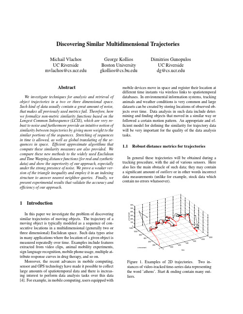
Discovering Similar Multidimensional TrajectoriesMichail VlachosUC Riverside mvlachos@George KolliosBoston Universitygkollios@Dimitrios GunopulosUC Riversidedg@AbstractWe investigate techniques for analysis and retrieval of object trajectories in a two or three dimensional space. Such kind of data usually contain a great amount of noise, that makes all previously used metrics fail.Therefore,here we formalize non-metric similarity functions based on the Longest Common Subsequence(LCSS),which are very ro-bust to noise and furthermore provide an intuitive notion of similarity between trajectories by giving more weight to the similar portions of the sequences.Stretching of sequences in time is allowed,as well as global translating of the se-quences in space.Efficient approximate algorithms that compute these similarity measures are also provided.We compare these new methods to the widely used Euclidean and Time Warping distance functions(for real and synthetic data)and show the superiority of our approach,especially under the strong presence of noise.We prove a weaker ver-sion of the triangle inequality and employ it in an indexing structure to answer nearest neighbor queries.Finally,we present experimental results that validate the accuracy and efficiency of our approach.1IntroductionIn this paper we investigate the problem of discovering similar trajectories of moving objects.The trajectory of a moving object is typically modeled as a sequence of con-secutive locations in a multidimensional(generally two or three dimensional)Euclidean space.Such data types arise in many applications where the location of a given object is measured repeatedly over time.Examples include features extracted from video clips,animal mobility experiments, sign language recognition,mobile phone usage,multiple at-tribute response curves in drug therapy,and so on.Moreover,the recent advances in mobile computing, sensor and GPS technology have made it possible to collect large amounts of spatiotemporal data and there is increas-ing interest to perform data analysis tasks over this data [4].For example,in mobile computing,users equipped with mobile devices move in space and register their location at different time instants via wireless links to spatiotemporal databases.In environmental information systems,tracking animals and weather conditions is very common and large datasets can be created by storing locations of observed ob-jects over time.Data analysis in such data include deter-mining andfinding objects that moved in a similar way or followed a certain motion pattern.An appropriate and ef-ficient model for defining the similarity for trajectory data will be very important for the quality of the data analysis tasks.1.1Robust distance metrics for trajectoriesIn general these trajectories will be obtained during a tracking procedure,with the aid of various sensors.Here also lies the main obstacle of such data;they may contain a significant amount of outliers or in other words incorrect data measurements(unlike for example,stock data which contain no errors whatsoever).Figure1.Examples of2D trajectories.Two in-stances of video-tracked time-series data representingthe word’athens’.Start&ending contain many out-liers.Athens 1Athens 2Boston 1Boston 2DTWLCSSFigure 2.Hierarchical clustering of 2D series (displayed as 1D for clariry).Left :The presence of many outliers in the beginning and the end of the sequences leads to incorrect clustering.DTW is not robust under noisy conditions.Right :The focusing on the common parts achieves the correct clustering.Our objective is the automatic classification of trajec-tories using Nearest Neighbor Classification.It has been shown that the one nearest neighbor rule has asymptotic er-ror rate that is at most twice the Bayes error rate[12].So,the problem is:given a database of trajectories and a query (not already in the database),we want to find the trajectory that is closest to .We need to define the following:1.A realistic distance function,2.An efficient indexing scheme.Previous approaches to model the similarity between time-series include the use of the Euclidean and the Dy-namic Time Warping (DTW)distance,which however are relatively sensitive to noise.Distance functions that are ro-bust to extremely noisy data will typically violate the trian-gular inequality.These functions achieve this by not consid-ering the most dissimilar parts of the objects.However,they are useful,because they represent an accurate model of the human perception,since when comparing any kind of data (images,trajectories etc),we mostly focus on the portions that are similar and we are willing to pay less attention to regions of great dissimilarity.For this kind of data we need distance functions that can address the following issues:Different Sampling Rates or different speeds.The time-series that we obtain,are not guaranteed to be the outcome of sampling at fixed time intervals.The sensors collecting the data may fail for some period of time,leading to inconsistent sampling rates.Moreover,two time series moving at exactly the similar way,but one moving at twice the speed of the other will result (most probably)to a very large Euclidean distance.Similar motions in different space regions .Objectscan move similarly,but differ in the space they move.This can easily be observed in sign language recogni-tion,if the camera is centered at different positions.If we work in Euclidean space,usually subtracting the average value of the time-series,will move the similar series closer.Outliers.Might be introduced due to anomaly in the sensor collecting the data or can be attributed to hu-man ’failure’(e.g.jerky movement during a track-ing process).In this case the Euclidean distance will completely fail and result to very large distance,even though this difference may be found in only a few points.Different lengths.Euclidean distance deals with time-series of equal length.In the case of different lengths we have to decide whether to truncate the longer series,or pad with zeros the shorter etc.In general its use gets complicated and the distance notion more vague.Efficiency.It has to be adequately expressive but suf-ficiently simple,so as to allow efficient computation of the similarity.To cope with these challenges we use the Longest Com-mon Subsequence (LCSS)model.The LCSS is a varia-tion of the edit distance.The basic idea is to match two sequences by allowing them to stretch,without rearranging the sequence of the elements but allowing some elements to be unmatched .The advantages of the LCSS method are twofold:1)Some elements may be unmatched,where in Eu-clidean and DTW all elements must be matched,even the outliers.2)The LCSS model allows a more efficient approximatecomputation,as will be shown later(whereas in DTW you need to compute some costly Norm).Infigure2we can see the clustering produced by the distance.The sequences represent data collected through a video tracking process.Originally they represent 2d series,but only one dimension is depicted here for clar-ity.The fails to distinguish the two classes of words, due to the great amount of outliers,especially in the begin-ning and in the end of the ing the Euclidean distance we obtain even worse results.The produces the most intuitive clustering as shown in the samefigure. Generally,the Euclidean distance is very sensitive to small variations in the time axis,while the major drawback of the is that it has to pair all elements of the sequences.Therefore,we use the model to define similarity measures for trajectories.Nevertheless,a simple extension of this model into2or more dimensions is not sufficient, because(for example)this model cannot deal with paral-lel movements.Therefore,we extend it in order to address similar problems.So,in our similarity model we consider a set of translations in2or more dimensions and wefind the translation that yields the optimal solution to the problem.The rest of the paper is organized as follows.In section2 we formalize the new similarity functions by extending the model.Section3demonstrates efficient algorithms to compute these functions and section4elaborates on the indexing structure.Section5provides the experimental validation of the accuracy and efficiency of the proposed approach and section6presents the related work.Finally, section7concludes the paper.2Similarity MeasuresIn this section we define similarity models that match the user perception of similar trajectories.First we give some useful definitions and then we proceed by presenting the similarity functions based on the appropriate models.We assume that objects are points that move on the-plane and time is discrete.Let and be two trajectories of moving objects with size and respectively,whereand.For a trajectory,let be the sequence.Definition1Given an integer and a real number,we define the as follows:A Ba and andThe constant controls how far in time we can go in order to match a given point from one trajectory to a point in another trajectory.The constant is the matching threshold(see figure3).Thefirst similarity function is based on the and the idea is to allow time stretching.Then,objects that are close in space at different time instants can be matched if the time instants are also close.Definition2We define the similarity function between two trajectories and,given and,as follows:Definition3Given,and the family of translations,we define the similarity function between two trajectories and,as follows:So the similarity functions and range from to. Therefore we can define the distance function between two trajectories as follows:Definition4Given,and two trajectories and we define the following distance functions:andNote that and are symmetric.is equal to and the transformation that we use in is translation which preserves the symmetric prop-erty.By allowing translations,we can detect similarities be-tween movements that are parallel in space,but not iden-tical.In addition,the model allows stretching and displacement in time,so we can detect similarities in move-ments that happen with different speeds,or at different times.Infigure4we show an example where a trajectory matches another trajectory after a translation is applied. Note that the value of parameters and are also important since they give the distance of the trajectories in space.This can be useful information when we analyze trajectory data.XFigure4.Translation of trajectory.The similarity function is a significant improvement over the,because:i)now we can detect parallel move-ments,ii)the use of normalization does not guarantee that we will get the best match between two u-ally,because of the significant amount of noise,the average value and/or the standard deviation of the time-series,that are being used in the normalization process,can be distorted leading to improper translations.3Efficient Algorithms to Compute the Simi-larity3.1Computing the similarity functionTo compute the similarity functions we have to run a computation for the two sequences.Thecan be computed by a dynamic programming algorithm in time.However we only allow matchings when the difference in the indices is at most,and this allows the use of a faster algorithm.The following lemma has been shown in[5],[11].Lemma1Given two trajectories and,with and,we canfind the in time.If is small,the dynamic programming algorithm is very efficient.However,for some applications may need to be large.For that case,we can speed-up the above computa-tion using random sampling.Given two trajectories and ,we compute two subsets and by sampling each trajectory.Then we use the dynamic programming algo-rithm to compute the on and.We can show that,with high probability,the result of the algorithm over the samples,is a good approximation of the actual value. We describe this technique in detail in[35].3.2Computing the similarity functionWe now consider the more complex similarity function .Here,given two sequences,and constants, we have tofind the translation that maximizes the length of the longest common subsequence of()over all possible translations.Let the length of trajectories and be and re-spectively.Let us also assume that the translationis the translation that,when applied to,gives a longest common subsequence,and it is also the translation that maximizes the length of the longest common subsequence.The key observation is that,although there is an infinite number of translations that we can apply to,each transla-tion results to a longest common subsequence between and,and there is afinite set of possible longest common subsequences.In this section we show that we can efficiently enumerate afinite set of translations,such that this set provably includes a translation that maximizes the length of the longest common subsequence of and .To give a bound on the number of transformations that we have to consider,we look at the projections of the two trajectories on the two axes separately.We define theprojection of a trajectoryto be the sequence of the valueson the -coordinate:.A one di-mensional translation is a function that adds a con-stant to all the elements of a 1-dimensional sequence:.Take the projections of and ,and respec-tively.We can show the following lemma:Lemma 2Given trajectories ,if ,then the length of the longest common subsequence of the one dimensional sequences and,is at least :.Also,.Now,consider and .A translation by ,applied to can be thought of as a linear transformation of the form .Such a transformation will allowto be matched to all for which ,and.It is instructive to view this as a stabbing problem:Con-sider the vertical line segments,where (Figure 5).Bx,i By,i+2Bx,i+3Bx,i+4Bx,i+5Ax,iAx,i+1Ax,i+2fc1(x) = x + c1fc2(x) = x + c2Ax axisBx axisFigure 5.An example of two translations.These line segments are on a two dimensional plane,where on the axis we put elements ofand on the axis we put elements of .For every pair of elementsin and that are within positions from eachother (and therefore can be matched by the algo-rithm if their values are within ),we create a vertical line segment that is centered at the point and extends above and below this point.Since each element in can be matched with at most elements in ,the total number of such line segments is .A translation in one dimension is a function of the form .Therefore,in the plane we de-scribed above,is a line of slope 1.After translatingby ,an element of can be matched to an el-ement of if and only if the line intersects the line segment .Therefore each line of slope 1defines a set of possi-ble matchings between the elements of sequences and.The number of intersected line segments is actually an upper bound on the length of the longest common sub-sequence because the ordering of the elements is ignored.However,two different translations can result to different longest common subsequences only if the respective lines intersect a different set of line segments.For example,the translations and in figure 5intersect different sets of line segments and result to longest common subsequences of different length.The following lemma gives a bound on the number of possible different longest common subsequences by bound-ing the number of possible different sets of line segments that are intersected by lines of slope 1.Lemma 3Given two one dimensional sequences ,,there are lines of slope 1that intersect different sets of line segments.Proof:Let be a line of slope 1.If we move this line slightly to the left or to the right,it still in-tersects the same number of line segments,unless we cross an endpoint of a line segment.In this case,the set of inter-sected line segments increases or decreases by one.There are endpoints.A line of slope 1that sweeps all the endpoints will therefore intersect at most different sets of line segments during the sweep.In addition,we can enumerate the trans-lations that produce different sets of potential matchings byfinding the lines of slope 1that pass through the endpoints.Each such translation corresponds to a line .This set of translations gives all possible matchings for a longest common subsequence of .By applying the same process on we can also find a set of translations that give all matchings of.To find the longest common subsequence of the se-quences we have to consider only thetwo dimensional translations that are created by taking the Cartesian product of the translations on and the trans-lations on .Since running the LCSS algorithm takeswe have shown the following theorem:Theorem 1Given two trajectories and,withand ,we can compute theintime.3.3An Efficient Approximate AlgorithmTheorem 1gives an exact algorithm for computing ,but this algorithm runs in cubic time.In this section we present a much more efficient approximate algorithm.The key in our technique is that we can bound the difference be-tween the sets of line segments that different lines of slope 1intersect,based on how far apart the lines are.Consider again the one dimensional projections. Lets us consider the translations that result to different sets of intersected line segments.Each translation is a line of the form.Let us sort these trans-lations by.For a given translation,let be the set of line segments it intersects.The following lemma shows that neighbor translations in this order intersect similar sets of line segments.Lemma4Let be the different translations for sequences and,where.Then the symmetric difference.We can now prove our main theorem:Theorem2Given two trajectories and,with and,and a constant,we canfind an ap-proximation of the similaritysuch that intime.Proof:Let.We consider the projections of and into the and axes.There exists a translation on only such that is a superset of the matches in the optimal of and.In addition,by the previous lemma,there are translations()that have at most different matchings from the optimal. Therefore,if we use the translations,fortime if we runpairs of translations in the plane.Since there is one that is away from the optimal in each dimension,there is one that is away from the optimal in2dimensions.Setting-th quantiles for each set,pairs of translations.4.Return the highest result.4Indexing Trajectories for Similarity Re-trievalIn this section we show how to use the hierarchical tree of a clustering algorithm in order to efficiently answer near-est neighbor queries in a dataset of trajectories.The distance function is not a metric because it does not obey the triangle inequality.Indeed,it is easy to con-struct examples where we have trajectories and, where.This makes the use of traditional indexing techniques diffi-cult.We can however prove a weaker version of the triangle inequality,which can help us avoid examining a large por-tion of the database objects.First we define:Clearly,or in terms of distance:In order to provide a lower bound we have to maximize the expression.Therefore,for every node of the tree along with the medoid we have to keep the trajectory that maximizes this expression.If the length of the query is smaller than the shortest length of the trajec-tories we are currently considering we use that,otherwise we use the minimum and maximum lengths to obtain an approximate result.4.2Searching the Index tree for Nearest Trajec-toriesWe assume that we search an index tree that contains tra-jectories with minimum length and maximum length .For simplicity we discuss the algorithm for the1-Nearest Neighbor query,where given a query trajectory we try tofind the trajectory in the set that is the most sim-ilar to.The search procedure takes as input a nodein the tree,the query and the distance to the closest tra-jectory found so far.For each of the children,we check if the child is a trajectory or a cluster.In case that it is a trajectory,we just compare its distance to with the current nearest trajectory.If it is a cluster,we check the length of the query and we choose the appropriate value for .Then we compute a lower bound to the distance of the query with any trajectory in the cluster and we compare the result with the distance of the current near-est neighbor.We need to examine this cluster only if is smaller than.In our scheme we use an approximate algorithm to compute the.Consequently,the value offrom the bound we compute for.Note that we don’t need to worry about the other terms since they have a negative sign and the approximation algorithm always underestimates the .5Experimental EvaluationWe implemented the proposed approximation and index-ing techniques as they are described in the previous sec-tions and here we present experimental results evaluating our techniques.We describe the datasets and then we con-tinue by presenting the results.The purpose of our experi-ments is twofold:first,to evaluate the efficiency and accu-racy of the approximation algorithm presented in section3 and second to evaluate the indexing technique that we dis-cussed in the previous section.Our experiments were run on a PC AMD Athlon at1GHz with1GB RAM and60 GB hard disk.5.1Time and Accuracy ExperimentsHere we present the results of some experiments using the approximation algorithm to compute the similarity func-tion.Our dataset here comes from marine mammals’satellite tracking data.It consists of sequences of geo-graphic locations of various marine animals(dolphins,sea lions,whales,etc)tracked over different periods of time, that range from one to three months(SEALS dataset).The length of the trajectories is close to.Examples have been shown infigure1.In table1we show the computed similarity between a pair of sequences in the SEALS dataset.We run the exact and the approximate algorithm for different values of and and we report here some indicative results.is the num-ber of times the approximate algorithm invokes the procedure(that is,the number of translations that we try).As we can see,for and we get very good results.We got similar results for synthetic datasets.Also, in table1we report the running times to compute the simi-larity measure between two trajectories of the same dataset. The approximation algorithm uses again from to differ-ent runs.The running time of the approximation algorithm is much faster even for.As can be observed from the experimental results,the running times of the approximation algorithm is not pro-portional to the number of runs().This is achieved by reusing the results of previous translations and terminat-ing early the execution of the current translation,if it is not going to yield a better result.The main conclusion of the above experiments is that the approximation algorithm can provide a very tractable time vs accuracy trade-off for computing the similarity between two trajectories,when the similarity is defined using the model.5.2Classification using the Approximation Algo-rithmWe compare the clustering performance of our method to the widely used Euclidean and DTW distance functions. Specifically:cover.htmlSimilarityApproximate for K tries Exact9494250.250.3160.18460.2530.00140.0022 0.50.5710.4100.5100.00140.0022 0.250.3870.1960.3060.00180.00281 0.50.6120.4880.5630.00180.00280 0.250.4080.2500.3570.001910.0031 0.50.6530.4400.5840.001930.0031 Table1.Similarity values and running times between two sequences from our SEALS dataset.1.The Euclidean distance is only defined for sequencesof the same length(and the length of our sequences vary considerably).We tried to offer the best possible comparison between every pair of sequences,by slid-ing the shorter of the two trajectories across the longer one and recording their minimum distance.2.For DTW we modified the original algorithm in orderto match both x and y coordinates.In both DTW and Euclidean we normalized the data before computing the distances.Our method does not need any normal-ization,since it computes the necessary translations.3.For LCSS we used a randomized version with andwithout sampling,and for various values of.The time and the correct clusterings represent the average values of15runs of the experiment.This is necessary due to the randomized nature of our approach.5.2.1Determining the values for&The values we used for and are clearly dependent on the application and the dataset.For most datasets we had at our disposal we discovered that setting to more than of the trajectories length did not yield significant improvement.Furthermore,after some point the similarity stabilizes to a certain value.The determination of is appli-cation dependent.In our experiments we used a value equal to the smallest standard deviation between the two trajec-tories that were examined at any time,which yielded good and intuitive results.Nevertheless,when we use the index the value of has to be the same for all pairs of trajectories.5.2.2Experiment1-Video tracking data.The2D time series obtained represent the X and Y position of a human tracking feature(e.g.tip offinger).In conjuc-tion with a”spelling program”the user can”write”various words[19].We used3recordings of5different words.The data correspond to the following words:’athens’,’berlin’,’london’,’boston’,’paris’.The average length of the series is around1100points.The shortest one is834points and the longest one1719points.To determine the efficiency of each method we per-formed hierarchical clustering after computing thepairwise distances for all three distance functions.We eval-uate the total time required by each method,as well as the quality of the clustering,based on our knowledge of whichword each trajectory actually represents.We take all possi-ble pairs of words(in this case pairs)and use the clustering algorithm to partition them into two classes.While at the lower levels of the dendrogram the clustering is subjective,the top level should provide an accurate divi-sion into two classes.We clustered using single,complete and average linkage.Since the best results for every dis-tance function are produced using the complete linkage,we report only the results for this approach(table2).The same experiment is conducted with the rest of the datasets.Exper-iments have been conducted for different sample sizes and values of(as a percentage of the original series length).The results with the Euclidean distance have many clas-sification errors and the DTW has some errors,too.For the LCSS the only real variations in the clustering are for sam-ple sizes.Still the average incorrect clusterings for these cases were constantly less than one().For 15%sampling or more,there were no errors.5.2.3Experiment2-Australian Sign LanguageDataset(ASL).The dataset consists of various parameters(such as the X,Y, Z hand position,azimuth etc)tracked while different writ-ers sign one the95words of the ASL.These series are rel-atively short(50-100points).We used only the X and Y parameters and collected5recordings of the following10 words:’Norway’,’cold’,’crazy’,’eat’,’forget’,’happy’,’innocent’,’later’,’lose’,’spend’.This is the experiment conducted also in[25](but there only one dimension was used).Examples of this dataset can be seen infigure6.Correct Clusterings(out of10)Complete Linkage Euclidean34.96DTW237.6412.7338.04116.17328.85145.06565.203113.583266.753728.277Distance Time(sec)CorrectClusterings(out of45)ASL with noiseEuclidean 2.271520Figure 7.ASL data :Time required to compute the pairwise distances of the 45combinations(same for ASL and ASL withnoise)Figure 8.Noisy ASL data :The correct clusterings of the LCSS method using complete linkage.Figure 9.Performance for increasing number of Near-est Neighbors.Figure 10.The pruning power increases along with the database size.jectories.We executed a set of -Nearest Neighbor (K-NN)queries for ,,,and and we plot the fraction of the dataset that has to be examined in order to guarantee that we have found the best match for the K-NN query.Note that in this fraction we included the medoids that we check during the search since they are also part of the dataset.In figure 9we show some results for -Nearest Neigh-bor queries.We used datasets with ,and clusters.As we can see the results indicate that the algorithm has good performance even for queries with large K.We also per-formed similar experiments where we varied the number of clusters in the datasets.As the number of clusters increased the performance of the algorithm improved considerably.This behavior is expected and it is similar to the behavior of recent proposed index structures for high dimensional data [9,6,21].On the other hand if the dataset has no clusters,the performance of the algorithm degrades,since the major-ity of the trajectories have almost the same distance to the query.This behavior follows again the same pattern of high dimensional indexing methods [6,36].The last experiment evaluates the index performance,over sets of trajectories with increasing cardinality.We in-dexed from to trajectories.The pruning power of the inequality is evident in figure 10.As the size of the database increases,we can avoid examining a larger frac-tion of the database.6Related WorkThe simplest approach to define the similarity between two sequences is to map each sequence into a vector and then use a p-norm distance to define the similarity measure.The p-norm distance between two n-dimensional vectors and is defined as。