2007 JCP Finite difference spectral approximations for the timefractional
- 格式:pdf
- 大小:364.96 KB
- 文档页数:20

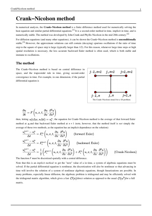
Crank –Nicolson methodIn numerical analysis, the Crank –Nicolson method is a finite difference method used for numerically solving the heat equation and similar partial differential equations.[1] It is a second-order method in time, implicit in time, and is numerically stable. The method was developed by John Crank and Phyllis Nicolson in the mid 20th century.[2]For diffusion equations (and many other equations), it can be shown the Crank –Nicolson method is unconditionally stable.[3] However, the approximate solutions can still contain (decaying) spurious oscillations if the ratio of time step to the square of space step is large (typically larger than 1/2). For this reason, whenever large time steps or high spatial resolution is necessary, the less accurate backward Euler method is often used, which is both stable and immune to oscillations.The methodThe Crank –Nicolson stencil for a 1D problem.The Crank –Nicolson method is based on central difference inspace, and the trapezoidal rule in time, giving second-orderconvergence in time. For example, in one dimension, if the partialdifferential equation isthen, letting , the equation for Crank –Nicolson method is the average of that forward Euler method at and that backward Euler method at n + 1 (note, however, that the method itself is not simply theaverage of those two methods, as the equation has an implicit dependence on the solution):The function F must be discretized spatially with a central difference.Note that this is an implicit method : to get the "next" value of u in time, a system of algebraic equations must be solved. If the partial differential equation is nonlinear, the discretization will also be nonlinear so that advancing in time will involve the solution of a system of nonlinear algebraic equations, though linearizations are possible. In many problems, especially linear diffusion, the algebraic problem is tridiagonal and may be efficiently solved with the tridiagonal matrix algorithm, which gives a fast direct solution as opposed to the usual for a full matrix.Example: 1D diffusionThe Crank–Nicolson method is often applied to diffusion problems. As an example, for linear diffusion,whose Crank–Nicolson discretization is then:or, letting :which is a tridiagonal problem, so that may be efficiently solved by using the tridiagonal matrix algorithm infavor of a much more costly matrix inversion.A quasilinear equation, such as (this is a minimalistic example and not general)would lead to a nonlinear system of algebraic equations which could not be easily solved as above; however, it ispossible in some cases to linearize the problem by using the old value for , that is instead of . Other times, it may be possible to estimate using an explicit method and maintain stability.Example: 1D diffusion with advection for steady flow, with multiple channel connectionsThis is a solution usually employed for many purposes when there's a contamination problem in streams or rivers under steady flow conditions but information is given in one dimension only. Often the problem can be simplified into a 1-dimensional problem and still yield useful information.Here we model the concentration of a solute contaminant in water. This problem is composed of three parts: the known diffusion equation ( chosen as constant), an advective component (which means the system is evolving in space due to a velocity field), which we choose to be a constant Ux, and a lateral interaction between longitudinal channels (k).where C is the concentration of the contaminant and subscripts N and M correspond to previous and next channel. The Crank–Nicolson method (where i represents position and j time) transforms each component of the PDE into the following:Now we create the following constants to simplify the algebra:and substitute <1>, <2>, <3>, <4>, <5>, <6>, α, β and λ into <0>. We then put the new time terms on the left (j + 1) and the present time terms on the right (j) to get:To model the first channel, we realize that it can only be in contact with the following channel (M), so the expression is simplified to:In the same way, to model the last channel, we realize that it can only be in contact with the previous channel (N), so the expression is simplified to:To solve this linear system of equations we must now see that boundary conditions must be given first to the beginning of the channels:: initial condition for the channel at present time step: initial condition for the channel at next time step: initial condition for the previous channel to the one analyzed at present time step: initial condition for the next channel to the one analyzed at present time stepFor the last cell of the channels (z) the most convenient condition becomes an adiabatic one, soThis condition is satisfied if and only if (regardless of a null value)Let us solve this problem (in a matrix form) for the case of 3 channels and 5 nodes (including the initial boundary condition). We express this as a linear system problem:whereNow we must realize that AA and BB should be arrays made of four different subarrays (remember that only three channels are considered for this example but it covers the main part discussed above).andwhere the elements mentioned above correspond to the next arrays and an additional 4x4 full of zeros. Please note that the sizes of AA and BB are 12x12:,,,&The d vector here is used to hold the boundary conditions. In this example it is a 12x1 vector:To find the concentration at any time, one must iterate the following equation:Example: 2D diffusionWhen extending into two dimensions on a uniform Cartesian grid, the derivation is similar and the results may leadto a system of band-diagonal equations rather than tridiagonal ones. The two-dimensional heat equationcan be solved with the Crank–Nicolson discretization ofassuming that a square grid is used so that . This equation can be simplified somewhat by rearrangingterms and using the CFL numberFor the Crank–Nicolson numerical scheme, a low CFL number is not required for stability, however it is required fornumerical accuracy. We can now write the scheme as:Application in financial mathematicsFurther information: Finite difference methods for option pricingBecause a number of other phenomena can be modeled with the heat equation (often called the diffusion equation in financial mathematics), the Crank–Nicolson method has been applied to those areas as well.[4] Particularly, the Black-Scholes option pricing model's differential equation can be transformed into the heat equation, and thus numerical solutions for option pricing can be obtained with the Crank–Nicolson method.The importance of this for finance, is that option pricing problems, when extended beyond the standard assumptions (e.g. incorporating changing dividends), cannot be solved in closed form, but can be solved using this method. Note however, that for non-smooth final conditions (which happen for most financial instruments), the Crank–Nicolsonmethod is not satisfactory as numerical oscillations are not damped. For vanilla options, this results in oscillation inthe gamma value around the strike price. Therefore, special damping initialization steps are necessary (e.g., fully implicit finite difference method).References[1]Tuncer Cebeci (2002). Convective Heat Transfer (/?id=xfkgT9Fd4t4C&pg=PA257&dq="Crank-Nicolson+method"). Springer. ISBN 0966846141. .[2]Crank, J.; Nicolson, P. (1947). "A practical method for numerical evaluation of solutions of partial differential equations of the heatconduction type". Proc. Camb. Phil. Soc.43 (1): 50–67. doi:10.1007/BF02127704..[3]Thomas, J. W. (1995). Numerical Partial Differential Equations: Finite Difference Methods. Texts in Applied Mathematics. 22. Berlin, NewYork: Springer-Verlag. ISBN 978-0-387-97999-1.. Example 3.3.2 shows that Crank–Nicolson is unconditionally stable when applied to.[4]Wilmott, P.; Howison, S.; Dewynne, J. (1995). The Mathematics of Financial Derivatives: A Student Introduction (http://books.google.co.in/books?hl=en&q=The Mathematics of Financial Derivatives Wilmott&um=1&ie=UTF-8&sa=N&tab=wp). Cambridge Univ. Press.ISBN 0521497892. .External links•Module for Parabolic P.D.E.'s (/mathews/n2003/CrankNicolsonMod.html)Article Sources and Contributors7Article Sources and ContributorsCrank–Nicolson method Source: /w/index.php?oldid=442507644 Contributors: Albertod4, Argoreham, Axemanstan, Ben pcc, Berland, Brookie, Chadernook,Crougeaux, Cyktsui, Dicklyon, Fintor, JJL, Jitse Niesen, JohnCD, Keenan Pepper, Koavf, Mariocastrogama, Michael Hardy, Mild Bill Hiccup, MrOllie, Natalya, Oleg Alexandrov, Ovis23, Peak, Roadrunner, Roundhouse0, Salih, Taxman, Zylorian, 53 anonymous editsImage Sources, Licenses and ContributorsImage:Crank-Nicolson-stencil.svg Source: /w/index.php?title=File:Crank-Nicolson-stencil.svg License: Public Domain Contributors: Original uploader was Berland at en.wikipediaLicenseCreative Commons Attribution-Share Alike 3.0 Unported///licenses/by-sa/3.0/。

第59卷 第3期吉林大学学报(理学版)V o l .59 N o .32021年5月J o u r n a l o f J i l i nU n i v e r s i t y (S c i e n c eE d i t i o n )M a y2021研究简报d o i :10.13413/j .c n k i .jd x b l x b .2020423分数阶非线性迭代方程的周期解李翠英1,吴 睿2,程 毅1(1.渤海大学数学科学学院,辽宁锦州121013;2.长春财经学院数学教研部,长春130122)摘要:考虑一类C a p u t o 型分数阶导数意义下非线性迭代微分方程的周期问题,在非线性项满足单边L i p s c h t i z 条件下,应用L e r a y -S c h a u d e r 不动点定理和拓扑度理论,证明该类非线性分数阶迭代微分方程解的存在性和唯一性.关键词:存在性;唯一性;分数阶;迭代方程中图分类号:O 175.14 文献标志码:A 文章编号:1671-5489(2021)03-0555-04P e r i o d i c S o l u t i o n s f o r aF r a c t i o n a lN o n l i n e a r I t e r a t i v eE qu a t i o n s L IC u i y i n g 1,WU Ru i 2,C H E N G Y i 1(1.C o l l e g e o f M a t h e m a t i c a lS c i e n c e s ,B o h a i U n i v e r s i t y ,J i n z h o u 121013,L i a o n i n g Pr o v i n c e ,C h i n a ;2.D e p a r t m e n t o f M a t h e m a t i c s ,C h a n g c h u nU n i v e r s i t y o f F i n a n c e a n dE c o n o m i c s ,C h a n gc h u n 130122,C h i n a )A b s t r a c t :W e c o n s ide r e d t h e p e r i o d i c p r o b l e m of ac l a s so fn o n l i n e a r i t e r a t i v ed i f f e r e n t i a l e qu a t i o n i n t h es e n s eo fC a p u t ot y p ef r a c t i o n a ld e r i v a t i v e .U n d e ro n es i d e d -L i p s c h t i zc o n d i t i o n so n n o n l i n e a r t e r m ,t h ee x i s t e n c ea n d u n i qu e n e s s o fs o l u t i o nf o rt h e n o n l i n e a rf r a c t i o n a li t e r a t i v e d i f f e r e n t i a l e q u a t i o n s i s p r o v e d b y a p p l y i n g t h eL e r a y -S c h a u d e r f i x e d p o i n t t h e o r e ma n d t o p o l o g i c a l d e g r e e t h e o r y .K e y w o r d s :e x i s t e n c e ;u n i q u e n e s s ;f r a c t i o n a l o r d e r ;i t e r a t i v e e q u a t i o n 收稿日期:2020-12-18. 网络首发日期:2021-04-06.第一作者简介:李翠英(1983 ),女,汉族,硕士,讲师,从事分数阶微分动力系统的研究,E -m a i l :l n c y999@126.c o m.通信作者简介:吴 睿(1978 ),女,汉族,博士,教授,从事微分方程理论的研究,E -m a i l :w u r u i 0221@s i n a .c o m.基金项目:吉林省自然科学基金(批准号:20200201274J C ).网络首发地址:h t t ps ://k n s .c n k i .n e t /k c m s /d e t a i l /22.1340.O.20210406.0958.001.h t m l .0 引 言目前,关于迭代微分方程的边值㊁周期问题研究已得到广泛关注.P e t u k h o v [1]研究了如下二阶迭代微分方程周期边值问题:x ᵡ=λx (x (t)),x (0)=x (T )=α,得到了参数λ,α在不同范围内方程解的存在唯一性;K a u f m a n n [2]考虑一类二阶迭代微分方程的边值问题,用S c h a u d e r 不动点定理证明了该问题解的存在性;文献[3-6]用不同的不动点理论(K r a s n o s e l s k i i 不动点定理㊁S c h a u d e r 不动点定理等)证明了若干类迭代微分方程周期解或拟周期解的存在唯一性.分数阶微分方程在数学㊁化学㊁物理和工程等许多领域应用广泛,但关于分数阶迭代微分方程边值㊁周期问题的研究成果目前报道较少.当非线性函数满足L i ps c h i t z 条件时,I b r a h i m 等[7]将整数阶的一些结果推广到分数阶迭代微分方程中.但目前已有结果均为处理一维的迭代微分系统,对于向量迭代方程的研究尚未见文献报道.本文在非线性函数满足单边L i p s c h i t z 条件时,证明一类非线性C a pu t o 型分数阶迭代向量微分系统周期解的存在唯一性.本文令Tʒ=[0,b],ℝn为n维E u c l i d空间,<㊃,㊃>表示ℝn中的内积, ㊃ 表示ℝn空间的范数.设C(T,ℝn)表示从T到ℝn全体连续函数组成的空间,其范数定义为 x C=m a x tɪT x(t) .关于分数阶微积分的基础知识可参见文献[8-9].1主要结果考虑如下分数阶迭代向量微分方程:C Dαx(t)+A x(t)=f(t,x(t),x[2]+(t)), x(0)=x(b),(1)其中:x[2]+(t)=(x1( x ),x2( x ), ,x n( x ));C Dαx(t)=1Γ(1-α)ʏt0(t-s)-αxᶄ(s)d s, ∀αɪ(0,1);A:ℝnңℝn是一个线性算子;f:Tˑℝnˑℝnңℝn是一个连续函数.下面给出假设条件:(H1)设A:ℝnңℝn是一个有界㊁线性的正定算子,即对任意的zɪℝn,存在常数cɪℝ+,使得<A z,z>ȡc z 2;(H2)设f:Tˑℝnˑℝnңℝn是一个连续函数,且:(i)对任意的u,vɪℝn,存在一个非负函数λɪLɕ+[0,b],使得∀tɪ[0,b], f(t,u,v) ɤλ(t);(i i)对任意的tɪ[0,b],u1,u2,v1,v2ɪℝn存在函数μɪLɕ+[0,b],使得<f(t,u1,v1)-f(t,u2,v2),u1-u2>ɤμ(t) u1-u2 2,其中 μ ɕ<c,c是H1中的常数.定理1假设条件(H1),(H2)成立,且b大于某常数M1/(1-α),则分数阶迭代微分系统(1)存在唯一解.证明:由文献[10]中推论7.1知,问题(1)等价于如下积分迭代方程:x(t)=Eα(A tα)x(0)+ʏt0(t-τ)α-1Eα,α(A(t-τ)α)f(τ,x(τ),x[2]+(τ))dτ.(2)定义算子T1:C(T,ℝn)ңC(T,ℝn),且T1(x(t))ʒ=Eα(A tα)x(0)+ʏt0(t-τ)α-1Eα,α(A(t-τ)α)f(τ,x,x[2]+)dτ.首先,证明解的先验有界性.根据算子T1的定义和假设条件(H2)中(i),可推出T1(x(t)) ɤ x(0) Eα(A Tα) +m a x tɪT Eα,α(A tα)Γ(α)ʏt0(t-s)α-1f(s,x(s),x[2](s))d sɤx(0) Mα+ λ ɕ^MαΓ(α)ʏt0(t-s)α-1d sɤx(0) Mα+ λ ɕ^MααΓ(α)bα,(3)其中Mα= Eα(A Tα) ,^Mα=m a x tɪT Eα,α(A tα) .下面估计初值 x(0) .在式(2)中令t=b,可得x(b)=Eα(A bα)x(0)+ʏb0(b-τ)α-1Eα,α(A(b-τ)α)f(τ,x(τ),x[2]+(τ))dτ.由x(0)=x(b)和假设条件(H1)易知,行列式E-Eα(A bα)ʂ0,其中E表示单位矩阵.故x(0)=(E-Eα(A bα))-1b0(b-τ)α-1Eα,α(A(b-τ)α)f(τ,x(τ),x[2]+(τ))dτ.655吉林大学学报(理学版)第59卷根据假设条件(H 2)中(i ),类似式(3),可得 x (0) ɤM E ^M α λ ɕb ααΓ(α),(4)其中M E = (E -E α(A b α))-1 .将式(4)代入式(3),可得 T 1(x (t )) ɤ(M E M α+1)^M α λ ɕαΓ(α)b α, ∀t ɪT .记M =(M E M α+1)^M α λ ɕαΓ(α),由于b >M 1/(1-α),因此 T 1(x (t )) ɤM b α<b .其次,证明非线性算子T 1是全连续算子,从而得到解的存在性.先证明∀x ɪC (T ,ℝn ),T 1(x (t ))ɪC (T ,ℝn ).对任意的t ,t +δɪ[0,b ],且δ>0,满足T 1(x (t +δ))-T 1(x (t ))=1Γ(α)ʏt +δ0(t +δ-s )α-1E α,α(A (t +δ-τ)α)f (s ,x (s ),x [2](s ))d s -1Γ(α)ʏt(t -s )α-1E α,α(A (t -τ)α)f (s ,x (s ),x [2](s ))d s +[E α(A (t +δ)α)-E α(A t α)]x (0)ɤ λ ɕ^M αΓ(α)ʏt +δ0(t +δ-s )α-1d s +ʏt 0(t +δ-s )α-1-(t -s )α-1d s +[E α(A (t +δ)α)-E α(A t α)]x (0)ɤ2 λ ɕ^M ααΓ(α)δα+2 λ ɕ^M ααΓ(α)(t +δ-a )α-(t -a )α+[E α(A (t +δ)α)-E α(A t α)]x (0).当δң0时,有T 1(x (t +δ))-T 1(x (t ))ң0,故T 1(x (t ))ɪC (T ,ℝn ).取x n ңx ɪC (T ,ℝn ),则易推出T 1(x n )-T 1(x )ң0,从而T 1:C (T ,ℝn )ңC (T ,ℝn )是连续的.根据1)中先验估计,应用A r z e l a -A s c o l i 定理易知,算子T 1:ΩңΩ是全连续的,其中Ωʒ={u ɪC (T ,ℝn ): u C ɤb +1}.从而可将微分迭代系统(1)解的存在性转化为T 1的不动点问题.定义映射h ε(x )=x -εT 1(x ),其中εɪ[0,1].取p ∉h (∂Ω),则对任意的εɪ[0,1],可得d e g (h ε,Ω,p )=d e g (h 1,Ω,p )=d e g (I -T 1,Ω,p )=d e g (h 0,Ω,p )=d e g (I ,Ω,p )=1ʂ0,其中I 是恒等映射.因此T 1在Ω上存在不动点,即x =T 1(x ).从而微分迭代系统(1)至少存在一个解.最后,证明微分迭代系统(1)解的唯一性.假设x 1,x 2ɪC (T ,ℝn )是问题(1)的两个解,对这两个解做差再与x 1-x 2做内积,可得<x 1(t )-x 2(t ),D α(x 1(t )-x 2(t ))>+<x 1(t )-x 2(t ),A (x 1(t )-x 2(t ))>=<x 1(t )-x 2(t ),f (t ,x 1(t ),x [2]1+(t ))-f (t ,x 2(t ),x [2]2+(t))>.根据假设条件(H 1)和(H 2)中(i i),利用分数阶微分不等式[10],可推出D α x 1(t )-x 2(t ) 2ɤ2<x 1(t )-x 2(t ),D α(x 1(t )-x 2(t ))>ɤ2μ(t ) x 1-x 2 2-2c x 1-x 2 2.(5)为方便,令S (t )= x 1(t )-x 2(t ) 2,式(5)可简化为D αS (t )ɤ2(μ(t )-c )S (t ),755 第3期 李翠英,等:分数阶非线性迭代方程的周期解855吉林大学学报(理学版)第59卷从而S(t)ɤS(0)Eα(2( μ ɕ-c)tα), ∀tɪT.再令t=b,得S(b)ɤS(0)Eα(2( μ ɕ-c)bα).(6)由S(t)= x1-x2 2及边界条件x(b)=x(0)可知,S(b)=S(0),整理可得S(0){1-Eα[2( μ ɕ-c)bα]}ɤ0.由M i t t a g-L e f f l e r函数Eα(t)(tȡ0)的单调性和 μ ɕ<c知,Eα[2( μ ɕ-c)bα]<1.又由S(0)= x1(0)-x2(0) 2ȡ0,可推出S(0)=0.由式(6)知,S(t)ɤ0,从而S(t)恒为0,即x1=x2,故迭代微分方程(1)有唯一解.参考文献[1] P E T U K HO V V R.O n a B o u n d a r y V a l u e P r o b l e m[J].T r u d y S e m T e o r D i f f e r e n c i a l U r a v n e n iǐO t k l o nA r g u m e n t o m U n i vD r užb y N a r o d o vP a t r i s aL u m u m b y,1965,3:252-255.[2] K A U F MA N N ER.E x i s t e n c e a n dU n i q u e n e s s o f S o l u t i o n s f o r aS e c o n d-O r d e r I t e r a t i v eB o u n d a r y-V a l u eP r o b l e m[J].E l e c t r o n i c JD i f f e r e n t i a l E q u a t i o n s,2018,2018(150):1-6.[3] Z HA O H Y,L I UJ.P e r i o d i cS o l u t i o n s o f a n I t e r a t i v eF u n c t i o n a lD i f f e r e n t i a l E q u a t i o nw i t hV a r i a b l eC o e f f i c i e n t s[J].M a t h M e t hA p p l S c i,2016,40(1):286-292.[4] B O U A K K A Z A,A R D J O U N I A,D J O U D I A.P e r i o d i c S o l u t i o n sf o ra S e c o n d O r d e r N o n l i n e a r F u n c t i o n a lD i f f e r e n t i a lE q u a t i o nw i t h I t e r a t i v eT e r m sb y S c h a u d e r sF i x e dP o i n tT h e o r e m[J].A c t a M a t hU n i vC o m e n i a n,2018,87(2):223-235.[5] L I UB W,T U NÇC.P s e u d oA l m o s tP e r i o d i cS o l u t i o n s f o r aC l a s s o fF i r s tO r d e rD i f f e r e n t i a l I t e r a t i v eE q u a t i o n s[J].A p p lM a t hL e t t,2015,40:29-34.[6] F E㊅C K A N M,WA N GJR,Z HA O H Y.M a x i m a l a n d M i n i m a lN o n d e c r e a s i n g B o u n d e dS o l u t i o n so f I t e r a t i v eF u n c t i o n a lD i f f e r e n t i a l E q u a t i o n s[J].A p p lM a t hL e t t,2021,113:106886-1-106886-7.[7]I B R A H I M R W,K I L IÇMA N A,D AMA G F H.E x i s t e n c ea n d U n i q u e n e s sf o raC l a s so f I t e r a t i v eF r a c t i o n a lD i f f e r e n t i a lE q u a t i o n s[J/O L].A d vD i f f e rE q u,2015-03-05[2017-11-10].h t t p s://d o i.o r g/10.1186/s13662-015-0421-y.[8] M I L L E R KS,R O S SB.A nI n t r o d u c t i o nt ot h eF r a c t i o n a lC a l c u l u sa n dF r a c t i o n a lD i f f e r e n t i a lE q u a t i o n s[M].N e w Y o r k:W i l e y,1993:80-121.[9] P O D L U B N Y I.F r a c t i o n a l D i f f e r e n t i a l E q u a t i o n s:A n I n t r o d u c t i o n t o F r a c t i o n a l D e r i v a t i v e s,F r a c t i o n a lD i f f e r e n t i a lE q u a t i o n s,t o M e t h o d s o fT h e i r S o l u t i o na n dS o m e o fT h e i rA p p l i c a t i o n s[M].S a nD i e g o:A c a d e m i cP r e s s,1998:41-119.[10] C H E NJJ,Z E N G Z G,J I A N G P.G l o b a l M i t t a g-L e f f l e rS t a b i l i t y a n d S y n c h r o n i z a t i o n o f M e m r i s t o r-B a s e dF r a c t i o n a l-O r d e rN e u r a lN e t w o r k s[J].N e u r a lN e t w,2014,51:1-8.(责任编辑:李琦)。

2007PLM征文之57:Feko在复杂目标RCS仿真计算中的应用1 前言计算复杂目标的雷达散射截面(RCS)对于国防、航空、航天、气象等各项事业都具有很重要的意义。
尤其在导弹系统的设计、仿真,雷达系统的设计、鉴定,无论在新装备的研制论证中,还是现预装备战术使用方案的制定等均需要复杂目标(如飞机、舰艇、导弹等)的RCS及其电磁散射特性[1]。
对于提高目标自身的生存能力以及隐身技术的研究以及对于目标的雷达探测和目标识别等,都具有重要的现实意义。
可节约大量经费和时间,具有重大的意义。
一般确定一个目标的RCS通常有二种方法,即理论仿真计算和试验测量[2]。
而仿真计算又分自行开发的软件和商业软件。
前者主要是指采用各种电磁理论算法如数值解法、高频解法和混合法等等[3] [4]。
如果要开发成功具有一定精度和速度的软件包也是有相当的难度。
后者主要是指Feko、Ansoft、cst 等一些商业软件包。
总之,电磁场仿真软件不仅可以部分或完全代替试验来获得目标的RCS,节省大量的人力、物力和财力,而且可以大大缩短产品研发时间,从而在雷达目标特性中得到广泛的应用。
由于在计算电大尺寸目标的RCS过程中,Feko具有一定的优势,因此本文着重介绍Feko软件以及采用它仿真计算的几个例子。
FEKO是基于严格的积分方程方法[5],用户无需对传播空间进行网格划分;由于积分方程基于格林函数构建,用户无需设置吸收边界条件;只要硬件条件许可,矩量法可以求解任意复杂结构的电磁问题。
对于超电大尺寸的问题,使用FEKO的混合方法来进行仿真模拟:对于关键性的部位使用矩量法,对其他重要的区域(一般都是大的平面或者曲面)使用PO或者UTD。
以全波分析技术—为矩量法(MoM)基础真正实现了MoM方法和PO/UTD的混合混合仿真技术降低了计算和存储量提供单机多CPU 、多机网络并行等程序版本、支持UNIX、Linux,满足工程需要。
MoM/PO/UTD方法可以输入高级CAD软件(如Pro/E等)创建的几何模型,再自动剖分网格。
混沌时间序列处理之第一步:相空间重构方法综述第1章相空间重构第1章相空间重构 (1)1.1 引言 (2)1.2 延迟时间τ的确定 (3)1.1.1自相关函数法 (4)1.1.2平均位移法 (4)1.1.3复自相关法 (5)1.1.4互信息法 (6)1.2嵌入维数m的确定 (7)1.2.1几何不变量法 (7)1.2.2虚假最近邻点法 (8)1.2.2伪最近邻点的改进方法-Cao方法 (9)1.3同时确定嵌入维和延迟时间 (10)1.3.1时间窗长度 (10)1.3.2 C-C方法 (10)1.3.3 改进的C-C方法 (12)1.3.4微分熵比方法 (14)1.4非线性建模与相空间重构 (14)1.5海杂波的相空间重构 (15)1.6本章小结 (16)1.7 后记 (16)参考文献 (17)1.1 引言一般时间序列主要是在时间域或变换域中进行研究,而在混沌时间序列处理中,无论是混沌不变量的计算、混沌模型的建立和预测都是在相空间中进行,因此相空间重构是混沌时间序列处理中非常重要的第一步。
为了从时间序列中提取更多有用信息,1980年Packard 等人提出了用时间序列重构相空间的两种方法:导数重构法和坐标延迟重构法[1]。
从原理上讲,导数重构和坐标延迟重构都可以用来进行相空间重构,但就实际应用而言,由于我们通常不知道混沌时间序列的任何先验信息,而且从数值计算的角度看,数值微分是一个对误差很敏感的计算问题,因此混沌时间序列的相空间重构普遍采用坐标延迟的相空间重构方法[2]。
坐标延迟法的本质是通过一维时间序列{()}x n 的不同时间延迟来构造m 维相空间矢量:{(),(),,((1))}x i x i x i m ττ=++?x(i) (1.1) 1981年Takens 等提出嵌入定理:对于无限长、无噪声的d 维混沌吸引子的标量时间序列{()}x n ,总可以在拓扑不变的意义上找到一个m 维的嵌入相空间,只要维数21m d ≥+[3]。
Finite difference/spectral approximations for the time-fractional diffusion equation qYumin Lin,Chuanju Xu*School of Mathematical Sciences,Xiamen University,361005Xiamen,ChinaReceived 9October 2006;received in revised form 18January 2007;accepted 2February 2007Available online 14February 2007AbstractIn this paper,we consider the numerical resolution of a time-fractional diffusion equation,which is obtained from the standard diffusion equation by replacing the first-order time derivative with a fractional derivative (of order a ,with 06a 61).The main purpose of this work is to construct and analyze stable and high order scheme to efficiently solve the time-fractional diffusion equation.The proposed method is based on a finite difference scheme in time and Legendre spectral methods in space.Stability and convergence of the method are rigourously established.We prove that the full dis-cretization is unconditionally stable,and the numerical solution converges to the exact one with order O ðD t 2Àa þN Àm Þ,where D t ;N and m are the time step size,polynomial degree,and regularity of the exact solution respectively.Numerical experiments are carried out to support the theoretical claims.Ó2007Elsevier Inc.All rights reserved.AMS Classification:65M12;65M06;65M70;35S10Keywords:Fractional diffusion equation;Spectral approximation;Stability;Convergence1.IntroductionThe use of fractional partial differential equations (FPDEs)in mathematical models has become increas-ingly popular in recent years.Different models using FPDEs have been proposed [4,14,16],and there has been significant interest in developing numerical schemes for their solution.Roughly speaking,FPDEs can be classified into two principal kinds:space-fractional differential equation and time-fractional one.One of the simplest examples of the former is fractional order diffusion equations,which are generalizations of classical diffusion equations,treating super-diffusive flow processes.Much of0021-9991/$-see front matter Ó2007Elsevier Inc.All rights reserved.doi:10.1016/j.jcp.2007.02.001qThis work was partially supported by National NSF of China under Grant 10531080,973High Performance Scientific Computation Research Program 2005CB321703,and Program of 985Innovation Engineering on Information in Xiamen University.*Corresponding author.Tel.:+865922580713;fax:+865922580608.E-mail address:cjxu@ (C.Xu).Journal of Computational Physics 225(2007)1533–1552/locate/jcpthe work published to date has been concerned with this kind of FPDEs(see e.g.[1,4–7,13,15,20]for a non-exhaustive list of references).In this paper,we consider the time-fractional diffusion equation(TFDE),obtained from the standard dif-fusion equation by replacing thefirst-order time derivative with a fractional derivative of order a,with 06a61.Time-fractional diffusion or wave equations are derived by considering continuous time random walk problems,which are in general non-Markovian processes.The physical interpretation of the fractional derivative is that it represents a degree of memory in the diffusing material[9].These models have been inves-tigated in analytical and numerical frames by a number of authors[8,11,18,19,21].Some of these authors have tried to construct analytical solutions to problems of time-fractional differential equations.For example, Schneider and Wyss[18]and Wyss[21]considered the time-fractional diffusion-wave equations.The corre-sponding Green functions and their properties are obtained in terms of Fox functions.Gorenflo et al.[8,9] used the similarity method and the method of Laplace transform to obtain the scale-invariant solution of TFDE in terms of the wright function.A similar construction of the solution to the time-fractional advec-tion–dispersion equations or TFDE in whole-space and half-space has been given in[10,11]by using the Fou-rier–Laplace transforms.However,published papers on the numerical solution of the TFDE equations are very sparse.Liu et al.[12] use afirst-orderfinite difference scheme in both time and space directions for this equation,where some sta-bility conditions are derived.Herein,we examine a practicalfinite difference/Legendre spectral method to solve the initial-boundary value time-fractional diffusion problem on afinite domain.An approach based on the backward differentiation combined with spatial collocation method is used to obtain estimates of (2-a)-order convergence in time and exponential convergence in space.It is also shown that the time-stepping scheme is unconditionally stable for all a2½0;1 .A series of numerical examples is presented and compared with the exact solutions to support the theoretical claims.Let us emphasize that the computation of the numerical solution of time-fractional differential equations has been generally limited to simple cases(low spatial dimension or small time integration)due to the‘‘glo-bal dependence’’ually,by the definition of the fractional derivative,the solution at a time t k depends on the solutions at all previous time levels t<t k.The fact that all previous solutions have to be saved to compute the solution at the current time level would make the storage very expensive if low-order methods are employed for spatial discretization.Contrarily,use of the spectral method can relax this stor-age limit because,as compared to a low-order method,the spectral method needs fewer grid points to pro-duce highly accurate solution.This is one of main advantages of the spectral method for FPDES.Another difficult point in solving TFDE lies in the discretization of the time-fractional derivative.The fact that the time-fractional derivative uses Caputo integral makes the standard schemes and corresponding numerical analysis not applicable.One of our main goals here is to propose an approach and provide an error analysis for this problem.The outline of the paper is as follows:first,we provide in Section2an analytical solution of the TFDE in a bounded domain.Second,afinite difference scheme for temporal discretization of this problem is pro-posed in Section3,where the stability and convergence analysis is given.A detailed error analysis is car-ried out for the semi-discrete problem,showing that the temporal accuracy is of(2-a)-order.In Section4, we construct a Legendre spectral collocation method for the spatial discretization of the TFDE.Error esti-mates are provided for the full discrete problem.Finally numerical experiments are presented in Section5 which support the theoretical error estimates.Some concluding remarks are given in thefinal section.2.Analytical solution of the TFDE in a bounded domainIn this section,wefirst describe the problem of fractional differential equation studied in this paper,and present some analytical solutions which will be found helpful in the comprehension of the nature of such a problem.Let L>0;T>0;K¼ð0;LÞ,consider the time-fractional diffusion equation of the formo a uðx;tÞo t a Ào2uðx;tÞo x2¼fðx;tÞ;x2K;0<t6Tð2:1Þ1534Y.Lin,C.Xu/Journal of Computational Physics225(2007)1533–1552subject to the following initial and boundary conditions:uðx;0Þ¼gðxÞ;x2K;ð2:2Þuð0;tÞ¼uðL;tÞ¼0;06t6T;ð2:3Þwhere a is the order of the time-fractional derivative.Here,we consider the case06a61.o a uðx;tÞo t a in(2.1)isdefined as the Caputo fractional derivatives of order a[16],given byo a uðx;tÞo t a ¼1Cð1ÀaÞZ to uðx;sÞo sd sðtÀsÞa;0<a<1:ð2:4ÞWhen a¼1,Eq.(2.1)is the classical diffusion equation:o uðx;tÞo t Ào2uðx;tÞo x2¼fðx;tÞ;x2K;0<t6T;ð2:5Þwhile the case a¼0corresponds to the classical Helmholtz elliptic equation.In fact the time derivative of inte-ger order in(2.5)can be obtained by taking the limit a!1in(2.4).In the case0<a<1,the definition of the Caputo fractional derivatives uses the information of the stan-dard derivatives at all previous time levels(non-Markovian process).If f 0,then by applying thefinite sine and Laplace transforms to(2.1),the analytical solution for the problem(2.1)–(2.3)can be obtained[1]asuðx;tÞ¼2LX1n¼0E aðÀa2n2t aÞsinðanxÞZ LgðrÞsinðanrÞd r;ð2:6Þwhere a¼p andE aðzÞ¼X1m¼0z mCða mþ1Þis the Mittag–Leffler function.We list here some special Mittag–Leffler-type functions having explicit expressions as follows:E1ðÀzÞ¼eÀz;E2ðzÞ¼coshðffiffizpÞ;E12ðzÞ¼X1m¼0z mC mþ1ÀÁ¼e z2erfcðÀzÞ;where erfc(z)is the error function complement defined byerfcðzÞ¼1ffiffiffip pZ1zeÀt2d t:Although expressed in a compact form,we note that using(2.6)to compute the exact solution is gen-erally difficult(especially for large time)due to slow convergence of the series E aðzÞfor a2ð0;1Þand big z.The exact solutions for a number of a are plotted in Fig.1,showing the smoothness of the solu-tions.The regularity of these solutions can be analyzed by using some properties of the Mittag–Leffler function[2].In the analysis of the numerical method that follows,we will assume that problem(2.1)–(2.3)has a unique and sufficiently smooth solution.3.Discretization in time:afinite difference schemeIn order to simplify the notations and without lose of generality,we consider the case f 0in the scheme construction and its numerical analysis.First,we introduce afinite difference approximation to discretize the time-fractional derivative.Lett k:¼k D t,k¼0;1;...;K,where D t:¼TK is the time step.To motivate the construction of the scheme,weuse the following formulation:for all06k6KÀ1,Y.Lin,C.Xu/Journal of Computational Physics225(2007)1533–15521535o a u ðx ;t k þ1Þo t a ¼1C ð1Àa ÞX k j ¼0Z t j þ1t j o u ðx ;s Þo s d sðt k þ1Às Þa¼1C ð1Àa ÞX k j ¼0u ðx ;t j þ1ÞÀu ðx ;t j ÞD t Z t j þ1t jd s ðt k þ1Às Þa þr k þ1D t ;ð3:1Þwhere r k þ1D t is the truncation error.It can be verified that the truncation error takes the following form:r k þ1D t6c u 1C ð1Àa ÞX k j ¼0Z t j þ1t j t j þ1þt j À2s ðt k þ1Às Þa d s þO ðD t 2Þ"#;ð3:2Þwhere c u is a constant depending only on u .For the first term in RHS of (3.2),we have1C ð1Àa ÞX k j ¼0Z t j þ1t j t j þ1þt j À2sðt k þ1Às Þa d s¼À1C ð1Àa ÞX k j ¼011Àa ð2j þ1ÞD t 2Àa½ðk Àj Þ1Àa Àðk þ1Àj Þ1Àa þ1C ð1Àa ÞX k j ¼021Àa D t 2Àa ½ðj þ1Þðk Àj Þ1Àa Àj ðk þ1Àj Þ1Àaþ1C ð1Àa ÞX k j ¼02ð1Àa Þð2Àa ÞD t 2Àa ½ðk Àj Þ2Àa Àðk þ1Àj Þ2Àa ¼D t 2Àa C ð2Àa Þðk þ1Þ1Àa þ2ðk 1Àaþðk À1Þ1Àa þðk À2Þ1Àa þÁÁÁþ11Àa Þh i À2D t 2ÀaC ð3Àa Þðk þ1Þ2Àa ¼D t 2Àa C ð2Àa Þðk þ1Þ1Àa þ2ðk 1Àa þðk À1Þ1Àa þðk À2Þ1Àa þÁÁÁþ11Àa ÞÀ22Àa ðk þ1Þ2Àa!:LetS ðk Þ¼ðk þ1Þ1Àaþ2ðk 1Àa þðk À1Þ1Àaþðk À2Þ1ÀaþÁÁÁþ11Àa ÞÀ22Àaðk þ1Þ2Àa:Incidentally,we find that j S ðk Þj is bounded for all a 2½0;1 and all k P 1,as proven in the following lemma.1536Y.Lin,C.Xu /Journal of Computational Physics 225(2007)1533–1552Lemma3.1.For all a2½0;1 and all K P1,it holdsj SðKÞj6c;where c is a constant independent of a;K.Proof.First,for a¼0,a direct calculation shows SðKÞ¼0for all K P1.Now we prove the lemma for a2ð0;1 .It can be verified thatSðKÞ¼ðKþ1Þ1Àaþ2ðK1ÀaþðKÀ1Þ1ÀaþðKÀ2Þ1ÀaþÁÁÁþ11ÀaÞÀ22ÀaðKþ1Þ2Àa¼X Kk¼0a k;wherea k¼ðkþ1Þ1Àaþk1ÀaÀ22Àaððkþ1Þ2ÀaÀk2ÀaÞ:This observation leads us to prove that the series P1k¼0a k converges.It is well known that the seriesP1k¼11k bconverges for all b>1.By consequence,it suffices to prove j a k j61k1þa for big enough k.In fact we have,for k P2,j a k j¼k1Àa1þ1 k1Àaþ1À2k2Àa1þ1k2ÀaÀ1!¼k1Àa1þ1þð1ÀaÞ1kþð1ÀaÞðÀaÞ2!1k2þð1ÀaÞðÀaÞðÀaÀ1Þ3!1k3þÁÁÁÀ2k2ÀaÀ1þ1þð2ÀaÞ1kþð2ÀaÞð1ÀaÞ2!1kþð2ÀaÞð1ÀaÞðÀaÞ3!1kþð2ÀaÞð1ÀaÞðÀaÞðÀaÀ1Þ4!1kþÁÁÁ¼k1Àa12!À23!ð1ÀaÞðÀaÞ1kþ13!À24!ð1ÀaÞðÀaÞðÀaÀ1Þ1kþÁÁÁ6k1Àa 13!ð1ÀaÞa1k21þ2ðaþ1Þ41kþ3ðaþ1Þðaþ2Þ201k2þÁÁÁ613!ð1ÀaÞa1k1þa1þ1kþ1k2þÁÁÁ623!ð1ÀaÞa1k1þa61k1þa:The proof is completed.hMore precise bound of SðkÞcan be obtained by numerical computations.Indeed our numerical tests show thatÀ16SðkÞ60806a61;k¼1;2;...,as observed in Fig.2,where evolution of SðkÞas a function of k for several typical values of a is plotted in the leftfigure,while limit of SðkÞas k tends to infinity as a function of a is shown in the rightfigure.Y.Lin,C.Xu/Journal of Computational Physics225(2007)1533–15521537Using Lemma3.1,and taking into account the fact that1Cð2ÀaÞ62for all a2½0;1 ,we have1Cð1ÀaÞX kj¼0Z t jþ1t jt jþ1þt jÀ2sðt kþ1ÀsÞad s62D t2Àa:As a result,it holdsr kþ1 D t K cuD t2Àa:ð3:3ÞOn the other side,a straightforward calculation of thefirst term in RHS of(3.1)gives1Cð1ÀaÞX kj¼0uðx;t jþ1ÞÀuðx;t jÞD tZ t jþ1t jd sðt kþ1ÀsÞa¼1Cð1ÀaÞX kj¼0uðx;t jþ1ÞÀuðx;t jÞD tZ t kþ1Àjt kÀjd tt a¼1Cð1ÀaÞX kj¼0uðx;t kþ1ÀjÞÀuðx;t kÀjÞD tZ t jþ1t jd tt¼1Cð2ÀaÞX kj¼0uðx;t kþ1ÀjÞÀuðx;t kÀjÞD t aðjþ1Þ1ÀaÀj1Àah i:For the sake of simplification,let us introduce the notations b j:¼ðjþ1Þ1ÀaÀj1Àa;j¼0;1;...;k,and define the discrete fractional differential operator L atbyL a t uðx;t kþ1Þ:¼1Cð2ÀaÞX kj¼0b juðx;t kþ1ÀjÞÀuðx;t kÀjÞD t a:Then(3.1)readso a uðx;t kþ1Þo t a ¼L atuðx;t kþ1Þþr kþ1D t:ð3:4ÞUsing L at uðx;t kþ1Þas an approximation of o a uðx;t kþ1Þaleads to the followingfinite difference scheme to(2.1):L a t u kþ1ðxÞ¼o2u kþ1ðxÞo x2;k¼0;1;...;KÀ1;ð3:5Þwhere u kþ1ðxÞis an approximation to uðx;t kþ1Þ.By virtue of(3.3),this scheme is formally of(2-a)-order accu-racy.A rigorous analysis of the convergence rate will be provided later for both semi-discrete and full-discrete cases,where we will prove that the temporal accuracy of the scheme(3.5)is globally of order2-a.Scheme(3.5)can be rewritten into,with simplification by omitting the dependence of u kþ1ðxÞon x:b0u kþ1ÀCð2ÀaÞD t a o2u kþ1o x2¼b0u kÀX kj¼1b j½u kþ1ÀjÀu kÀj ¼b0u kÀX kÀ1j¼0b jþ1u kÀjþX kj¼1b j u kÀj:ð3:6ÞIt is worthwhile to noting that the second term in the RHS of(3.6)automatically vanishes when k61,while the last two terms of(3.6)vanish when k¼0.It is direct to check thatb j>0;j¼0;1;...;k;1¼b0>b1>ÁÁÁ>b k;b k!0as k!1;X k j¼0ðb jÀb jþ1Þþb kþ1¼ð1Àb1ÞþX kÀ1j¼1ðb jÀb jþ1Þþb k¼1:ð3:7ÞLet us introduce the parameter a0:a0:¼Cð2ÀaÞD t a;and note that b0¼1,then by reformulating the right-hand side of(3.6),we obtain an equivalent form to scheme(3.5):1538Y.Lin,C.Xu/Journal of Computational Physics225(2007)1533–1552u kþ1Àa0o2u kþ1o x2¼ð1Àb1Þu kþX kÀ1j¼1ðb jÀb jþ1Þu kÀjþb k u0;k P1:ð3:8ÞHere again,when k¼1scheme(3.8)becomesu2Àa0o2u2o x2¼ð1Àb1Þu1þb1u0:For the special case k¼0,that is thefirst time step,the scheme simply readsu1Àa0o2u1o x2¼u0:ð3:9ÞEqs.(3.8)and(3.9),together with the boundary conditionsu kþ1ð0Þ¼u kþ1ðLÞ¼0;k P0;ð3:10Þand the initial conditionu0ðxÞ¼gðxÞ;x2Kð3:11Þform a complete set of the semi-discrete problem.It will be useful to define the error term r kþ1byr kþ1:¼a0o a uðx;t kþ1Þo t aÀL atuðx;t kþ1Þ!:ð3:12ÞThen we have from(3.3)and(3.4)j r kþ1j¼Cð2ÀaÞD t a j r kþ1D tj6c u D t2:ð3:13ÞTo introduce the variational formulation of the problem(3.8),we define some functional spaces endowed with standard norms and inner products that will be used hereafter.H1ðKÞ:¼v2L2ðKÞ;d vd x2L2ðKÞ&';H10ðKÞ:¼v2H1ðKÞ;v jo K¼0ÈÉ;H mðKÞ:¼v2L2ðKÞ;d k vk2L2ðKÞfor all positive integer k6m&';where L2ðKÞis the space of measurable functions whose square is Lebesgue integrable in K.The inner products of L2ðKÞand H1ðKÞare defined,respectively,byðu;vÞ¼ZK uv d x;ðu;vÞ1¼ðu;vÞþd ud x;d vd xand the corresponding norms byk v k0¼ðv;vÞ1=2;k v k1¼ðv;vÞ1=21:The norm kÁkmof the space H mðKÞis defined byk v km ¼X mk¼0d k vd x k2!1=2:In this paper,instead of using the above standard H1-norm,we prefer to define kÁk1byk v k1¼k v k2þa0d ud x2!1=2:ð3:14ÞY.Lin,C.Xu/Journal of Computational Physics225(2007)1533–15521539It is well known that the standard H1-norm and the norm defined by(3.14)are equivalent,the latter will be used in what follows.The variational(weak)formulation of the Eq.(3.8)subject to the boundary condition(3.10)reads:find u kþ12H1ðKÞ,such thatðu kþ1;vÞþa0o u kþ1o x;o vo x¼ð1Àb1Þðu k;vÞþX kÀ1j¼1ðb jÀb jþ1Þðu kÀj;vÞþb kðu0;vÞ;8v2H1ðKÞ:ð3:15ÞFor this weak semi-discretized problem,we have the following stability result.Theorem3.1.The semi-discretized problem(3.15)is unconditionally stable in the sense that for all D t>0,it holdsk u kþ1k16k u0k;k¼0;1;...;KÀ1:Proof.We will prove the result by induction.First when k¼0,we haveðu1;vÞþa0o u1o x;o vo x¼ðu0;vÞ8v2H1ðKÞ:Taking v¼u1and using the inequality k v k06k v k1and Schwarz inequality,we obtain immediatelyk u1k16k u0k:Suppose now we have provenk u j k16k u0k;j¼1;2;...;k;ð3:16Þwe want to prove k u kþ1k16k u0k.Taking v¼u kþ1in(3.15)givesðu kþ1;u kþ1Þþa0o u kþ1;o u kþ1¼ð1Àb1Þðu k;u kþ1ÞþX kÀ1j¼1ðb jÀb jþ1Þðu kÀj;u kþ1Þþb kðu0;u kþ1Þ:Hence,by using(3.16),we havek u kþ1k216ð1Àb1Þk u k kk u kþ1kþX kÀ1j¼1ðb jÀb jþ1Þk u kÀj kk u kþ1kþb k k u0kk u kþ1k6½ð1Àb1ÞþX kÀ1j¼1ðb jÀb jþ1Þþb k k u0kk u kþ1k1:Finally,the last equality of(3.7)yieldsk u kþ1k16k u0k:ÃNow we carry out an error analysis for the solution of the semi-discretized problem.We denote from now by c a generic constant which may not be the same at different occurrences.Theorem3.2.Let u be the exact solution of(2.1)–(2.3),f u k g K k¼0be the time-discrete solution of(3.15)with the initial condition u0ðxÞ¼uðx;0Þ,then we have the following error estimates:(1)when06a<1,k uðt kÞÀu k k16cu;aT a D t2Àa;k¼1;2;...;K;ð3:17Þwhere c u;a:¼c u=ð1ÀaÞ,with c u:constant defined in(3.3);(2)when a!1,k uðt kÞÀu k k16cuT D t;k¼1;2;...;K:ð3:18Þ1540Y.Lin,C.Xu/Journal of Computational Physics225(2007)1533–1552Proof.(1)First consider the case06a<1.We start by proving the following estimate:k uðt jÞÀu j k16cubÀ1jÀ1D t2;j¼1;2;...;K:ð3:19ÞAs in the proof of Theorem3.1,we will use the mathematical induction.Let e k¼u x;t kðÞÀu kðxÞ.For j¼1,we have,by combining(2.1),(3.9)and(3.12),the error equation:ð e1;vÞþa0o e1o x;o vo x¼ð e0;vÞþðr1;vÞ¼ðr1;vÞ8v2H1ðKÞ:Taking v¼ e1yieldsk e1k216k r1kk e1k:This,together with(3.13),givesk uðt1ÞÀu1k16cubÀ1D t2:Therefore,(3.19)is proven for the case j¼1.Suppose now(3.19)holds for all j¼1;2;...;k,we need then to prove that it holds also for j¼kþ1.By combining(2.1),(3.12)and(3.15),we derive,8v2H1ðKÞð e kþ1;vÞþa0o e kþ1o x;o vo x¼ð1Àb1Þð e k;vÞþX kÀ1j¼1ðb jÀb jþ1Þð e kÀj;vÞþb kð e0;vÞþðr kþ1;vÞ:ð3:20ÞLet v¼ e kþ1in(3.20),thenk e kþ1k216ð1Àb1Þk e k kk e kþ1kþX kÀ1j¼1ðb jÀb jþ1Þk e kÀj kk e kþ1kþb k k e0kk e kþ1kþk r kþ1kk e kþ1k:Dividing by k e kþ1k1at both sides,using the induction assumption and the fact that bÀ1jbÀ1jþ1<1for all non-negativeinteger j,we obtaink e kþ1k16ð1Àb1ÞbÀ1kÀ1þX kÀ1j¼1ðb jÀb jþ1ÞbÀ1kÀjÀ1"#c u D t2þc u D t26ð1Àb1ÞþX kÀ1j¼1ðb jÀb jþ1Þþb k"#c u bÀ1kD t2:Using(3.7)in the above inequality givesk e kþ1k16cubÀ1kD t2:The estimate(3.19)is proved.Now,by the definition of b k,a direct computation shows thatkÀa bÀ1kÀ1¼kÀak1ÀaÀðkÀ1Þ!11Àa;as k!1;and the function/ðxÞ:¼xÀax1ÀaÀðxÀ1Þ1Àais increasing on x for all x>1since/0ðxÞ¼1xðxÀ1Þa1À1À1xaÀax!P08x>1;06a61:This means kÀa bÀ1kÀ1increasingly tends to11Àaas1<k!1.Note that kÀa bÀ1kÀ1¼1when k¼1,hence we havekÀa bÀ1kÀ1611Àa;k¼1;2;...;K:ð3:21ÞConsequently we obtain,for all k such that k D t6T,Y.Lin,C.Xu/Journal of Computational Physics225(2007)1533–15521541k uðt kÞÀu k k16cubÀ1kÀ1D t2¼c u kÀa bÀ1kÀ1k a D t26c u11Àaðk D tÞa D t2Àa6c u;a T a D t2Àa:(2)Now we consider the case a!1.Note that in this case,the estimate(3.17)has no meaning since c u;a tends to infinity as a!1.Therefore,we need to look for an estimate of other form.Taking into account the fact j D t6T for all j¼1;2;...;K,we are led to establish:k uðt jÞÀu j k16cuj D t2;j¼1;2;...;K:ð3:22ÞOnce again,we derive this estimate by induction.(3.22)is obvious for j¼1.Suppose now(3.22)holds for j¼1;2;...;k,we want to prove that it remains true for j¼kþ1.A similar procedure as in case(1)leads tok e kþ1k16ð1Àb1Þk e k kþX kÀ1j¼1ðb jÀb jþ1Þk e kÀj kþb k k e0kþk r kþ1k6ð1Àb1Þ½c u k D t2 þX kÀ1j¼1ðb jÀb jþ1Þ½c uðkÀjÞD t2 þc u D t2¼ð1Àb1Þkkþ1þX kÀ1j¼1ðb jÀb jþ1ÞkÀjkþ1þ1kþ1"#c uðkþ1ÞD t2¼ð1Àb1ÞþX kÀ1j¼1ðb jÀb jþ1ÞÀð1Àb1Þ1kþ1ÀX kÀ1j¼1ðb jÀb jþ1Þjþ1kþ1þ1kþ1"#c uðkþ1ÞD t2:ð3:23ÞIt is observed thatð1Àb1Þ1kþ1þX kÀ1j¼1ðb jÀb jþ1Þjþ1kþ1þb k P1kþ1ð1Àb1ÞþX kÀ1j¼1ðb jÀb jþ1Þþb k"#¼1kþ1;which is equivalent toÀð1Àb1Þ1kþ1ÀX kÀ1j¼1ðb jÀb jþ1Þjþ1kþ1þ1kþ16bk:Bringing this inequality into(3.23)givesk e kþ1k16ð1Àb1ÞþX kÀ1j¼1ðb jÀb jþ1Þþb k"#c uðkþ1ÞD t2¼c uðkþ1ÞD t2:Hence(3.22)is proven,i.e.(3.18)holds.The proof is completed.h4.Full discretization4.1.A Galerkin spectral method in spaceTo simplify the notations,we let K¼ðÀ1;1Þhereafter.The Galerkin spectral discretization proceeds by approximating the solution by the polynomials of high degree.To this end,we define P NðKÞthe space ofall polynomials of degree6N with respect to x.Then the discrete space,denoted by P0N ðKÞ,is defined as fol-lows:P0N ðKÞ:¼H1ðKÞ\P NðKÞ.Now consider the spectral discretization to the problem(3.15)as follows:find u kþ1N 2P0NðKÞ,such that forall v N2P0NðKÞðu kþ1N ;v NÞþa0oo xu kþ1N;oo xv N¼ð1Àb1Þðu kN;v NÞþX kÀ1j¼1ðb jÀb jþ1Þðu kÀj N;v NÞþb kðu0N;v NÞ:ð4:1ÞFor f u jN g kj¼0given,the well-posedness of the problem(4.1)is guaranteed by the well-known Lax–MilgramLemma.We are interested in this section in deriving an error estimate for the full-discrete solution f u kN g K k¼0.1542Y.Lin,C.Xu/Journal of Computational Physics225(2007)1533–1552。