Slow Roll Reconstruction Constraints on Inflation from the 3 Year WMAP Dataset

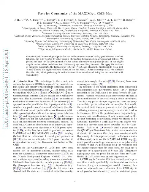
a r X i v :a s t r o -p h /0104248v 1 15 A p r 2001Tests for Gaussianity of the MAXIMA-1CMB MapJ.H.P.Wu 1,A.Balbi 2,3,4,J.Borrill 3,5,P.G.Ferreira 6,S.Hanany 3,7,A.H.Jaffe 1,3,8,A.T.Lee 3,4,9,B.Rabii 3,9,P.L.Richards 3,9,G.F.Smoot 3,4,8,9,R.Stompor 3,8,10,C.D.Winant 3,91Dept.of Astronomy,University of California,Berkeley,CA94720-3411,USA2Dipartimento di Fisica,Universit`a Tor Vergata,Roma,Via della Ricerca Scientifica,I-00133,Roma,Italy3Center for Particle Astrophysics,University of California,Berkeley,CA94720-7304,USA4Lawrence Berkeley National Laboratory,Berkeley,CA94720,USA5National Energy Research Scientific Computing Center,Lawrence Berkeley National Laboratory,Berkeley,CA94720,USA6Astrophysics,University of Oxford,Oxford,OX13RH,UK7School of Physics and Astronomy,University of Minnesota/Twin Cities,Minneapolis,MN55455,USA8Space Sciences Laboratory,University of California,Berkeley,CA94720,USA 9Dept.of Physics,University of California,Berkeley,CA94720-7300,USA 10Copernicus Astronomical Center,Bartycka 18,00-716Warszawa,PolandGaussianity of the cosmological perturbations in the universe is one of the key predictions of standard inflation,but it is violated by other models of structure formation such as topological defects.We present the first test of the Gaussianity of the cosmic microwave background (CMB)on sub-degree angular scales,where deviations from Gaussianity are most likely to occur.We apply the methods of moments,cumulants,the Kolmogorov test,the χ2test,and Minkowski functionals in eigen,real,Wiener-filtered and signal-whitened spaces,to the MAXIMA-1CMB anisotropy data.We conclude that the data,which probe angular scales between 10arcminutes and 5degrees,are consistent with Gaussianity.A.Introduction :The anisotropy in the cosmic mi-crowave background (CMB)is arguably the cleanest cos-mic signal that preserves the intrinsic statistical proper-ties of cosmological perturbations [1].The recent obser-vations from MAXIMA-1[2]and BOOMERANG [3]have unambiguously detected a sharp peak in the CMB power spectrum.This has favored inflation [4]as the dominant mechanism for structure formation of the universe [5]as opposed to other candidates like topological defects [6].Another key prediction of standard inflation is that the distribution of cosmic perturbations are Gaussian,while other cosmological models such as isocurvature inflation (e.g.[7])and topological defects (e.g.[8])predict other-wise.Thus tests for the Gaussianity of CMB anisotropy data can discriminate between cosmological models.In addition,a Gaussian distribution is an important ingre-dient in the estimation algorithm of CMB power spec-tra [9,10],which has been used to produce the recent MAXIMA-1and BOOMERANG results [2,3].Adding the fact that the estimation of cosmological parameters [11–13]relies on the estimated CMB power spectra,it is important to verify the Gaussian distribution of the CMB.Tests for the Gaussianity of CMB data have been carried out by numerous authors,mainly using data from the Differential Microwave Radiometer (DMR)on the COsmic Background Explorer (COBE)[14].Sev-eral statistics were used including moments,cumulants,Minkowski functionals (which include genus,e.g.[15,16]),the three-point function (e.g.[17]),bispectrum (e.g.[18,19]),wavelet transform (e.g.[20]),etc.All these tests showed that the data were consistent with Gaussianity,except for a couple of results [19,20]that may have non-cosmological origins [21].In addition to the usual limitations from foreground contamination and instrumental noise,the 7◦angular resolution of the DMR data is not ideal for tests of Gaus-sianity.Angular resolution is an issue because the size of the causal horizon at last scattering is about one degree.Thus in a sky patch of super-degree size,there are many uncorrelated perturbations due to causality.As a result,the central limit theorem guarantees that the pre-last-scattering anisotropy on super-degree scales will tend to be Gaussian.Even if the post-last-scattering anisotropy is strong and non-Gaussian,it can be obscured by the pre-last-scattering contribution,which we expect to be Gaussian.Therefore a CMB map with sub-degree reso-lution can provide much more powerful tests for Gaus-sianity.Park et al.[22]recently used a genus test on the QMAP and Saskatoon data,which have a resolution of about 1.5◦,to show that they were consistent with Gaussianity.In this paper we report results from a series of Gaussianity tests on the MAXIMA-1CMB map [2],which provides anisotropy information on angular scales between 10′and 5◦.To optimize both the resolution and the signal-to-noise ratio for these tests,we shall use a map with 5972square pixels of 8′each [23].Using these high-quality data we probe for the first time the Gaus-sianity of CMB anisotropy on sub-degree scales.A CMB sky is Gaussian if it is a realization of a pro-cess that is only specified by the two-point correlation function of a given cosmological model.However,be-cause we have only one realization of the CMB sky,it is not possible to exhaustively test the statistical prop-erties of the process that generated it.Therefore,we employ a Frequentist approach,testing the null hypoth-esis of Gaussianity for the inflationary model that best fits the data.B.Karhunen-Lo`e ve transform :We consider the Karhunen-Lo`e ve (K-L)transform,sometimes called Prin-cipal ComponentAnalysis or the signal-to-noise eigen-mode transformation [24,9],because it enables us not only to transform the observed CMB map into uncor-related eigenmodes of known signal-to-noise ratios,and further to implement Gaussianity tests on the uncorre-lated modes.For the CMB,it is standard to model the data d ≡d i as a linear sum of uncorrelated signal s ≡s i and noise n ≡n i ,with the correlation matrix C ≡ dd T =S +N where S = ss T and N = nn T .In the noise-whitened space d (W)=N −1/2d ,all the eigenvalues of the noise matrix,N −1/2NN −1/2=I ,are simply unity.Thus the eigenvalues e S (W)of the noise-whitened signal matrix N −1/2SN −1/2represent the square of signal-to-noise ratios of each eigenmode.The coefficients b (W)of the noise-whitened eigenmodes in a data set can be obtained by transforming d (W)to the ba-sis which diagonalizes N −1/2CN −1/2.These coefficients are normally called the K-L coefficients.We compute S using the CMB power spectrum of the best estimated cosmological model [11](Ωb =0.105,Ωc =0.595,ΩΛ=0.3,and h =0.53)and including the effects introduced by the beam shape and the pixelization of the map [25].The matrix N is estimated from the tem-poral data [23].The resulting eigenvalues in the noise-whitened space are shown in Fig.1,sorted in descending order.The dot-dashed line indicates that only the first639modes have signal-to-noise ratios e S (W) 1/2≥1.This number is well below our pixel number 5972.It is determined by the signal and noise levels and the observ-ing resolution (beam)of a data set,but is independent of the pixel number of the map when the pixel size is not larger than the observing resolution.A common technique to remove the information of non-cosmological interest in the map is Wiener filtering,d WF =SC −1d .This is equivalent to weighting the eigen-modes with the ratios e S (W)/(e S (W)+1)(see Fig.1).The sum of these ratios for all the eigenmodes is 837,again well below the total number 5972of the eigenmodes.We shall employ this technique in section D to amplify the statistical significance of the CMB signal in our map.The K-L transform can also be used to test for Gaussianity.If the underlying map is Gaussian,then the eigenvalue-normalized K-L coefficients a (W)≡b (W)/(e S (W)+1)1/2should be a set of Gaussian variables with mean zero and variance one.We compute the a (W)of our data,and use the observed frequency distribu-tion to approximate its one-point probability distribution functions (PDF)p (ν),where νis the number of standard deviations from the mean,for both the entire 5972andCMB data (top),and the Wiener filter (bottom).(b)a (W)of the MAXIMA-1data (solid),the Gaussian expec-tation (dashed),and its 95%CRG (shaded).the first 639modes (i.e.,those modes with signal domi-nating over noise).Both cases easily pass the χ2and the Kolmogorov tests for Gaussianity at 95%confidence.In addition to the above tests,we also use Monte Carlo (MC)simulation to build a Gaussian reference frame for the Frequentist approach.We generate 100,000Gaussianrealizations,each of which is obtained by d MC i=C 1/2ij g j ,where g j is a Gaussian variable of mean zero and variance one.As a first application,we use the MC simulation to find the probability distribution of p (ν)at each νfor the entire 5972and the first 639a (W).Fig.2shows that in both cases the real data lie well within the 95%confidence regions of Gaussianity (hereafter CRG).We also compute the moments and cumulants of the first 639a (W)up to tenth order,and they are all well within the 99%CRG.All these results support the conclusions not only that our map is consistent with Gaussianity,but also that our estimations of noise and CMB power spectrum (giving N and S respectively)are consistent with the data so as to provide the proper eigenmodes for the K-L transform.C.Minkowski functionals :The concept of Minkowski functionals is based on integral geometry.According to Hadwiger’s Theorem β+1Minkowski functionals are suf-ficient to measure the morphology of a β-dimensional pattern.In the case of CMB we have β=2and thus need only three Minkowski Functionals.First we de-fine the excursion set Q in a given CMB field as the region in which the CMB amplitude d i is larger than a threshold:Q ≡Q (ν)={d i |(d i −µ)/σ>ν},where µ= d and σ2= d 2 −µ2.Then the surface densities v i (ν)≡V i (Q )/A of Minkowski functionals V i (Q )for aan offset in the pixel positions every other row.(b)An example of a pixelized CMB map with the artificial pixel offset. CMB patch of angular area A can be defined asv0=14A∂Qdl,v2=12)/2,v1(G)=τ1/2exp(−ν2/2)/8σ,and v2(G)=τνexp(−ν2/2)/(2π)3/2σ2.We also note that the com-monly used one-point PDF p(ν)and genus g,or the‘Euler-Poincar´e characteristics’,are simply related to the Minkowski Functionals.For the two-dimensional CMB,we have p(ν)=−∂V0/A∂νand g=V2+V0/2π. Because the MAXIMA-1map has an irregular bound-ary and all pixels have a square shape lying on a regularlattice,we need a numerical scheme to approximate its Minkowski Functionals.For a given thresholdνand thusa given Q on the lattice,v0is simply the number of pixelsin Q divided by the total number of pixels in the map. Here v1is determined by the length of∂Q multipliedbyπ/4to correct for the square-pixel lattice effect.To compute v2,wefirst induce offset in the pixel positionsevery other row.As Fig.3(a)shows,this gives two types(I and II)of vertices.For each type,the integration of κin equation(1)can be easily obtained by examiningthe status of the neighboring four pixels(basically theintegration is determined by the change of the internal angle along∂Q).Fig.3(b)shows an example,where thepixels in Q are shaded and the one with no CMB data is labeled with a cross.In this case the verticesα1,α2,α3andα4have unambiguously αi(2κ/π)dl=−2,2,−1 and0respectively,while a confusion in this calculation would occur atα1andα2if there was no offset every otherrow.We also notice that any bias possibly induced bythe above algorithms should disappear when the number of pixels is large,as in our case.We compute the v0(ν),v1(ν),and v2(ν)for both the entire map and the central37%(2209pixels,coveringIMA-1map(a)and the central part(b).The Gaussian ex-pectation obtained from the MC simulation(dashed),its95% CRG(shaded),and the analytic Gaussian forms(dotted). about6.3◦×6.3◦),expected to have the lowest noise.We use pixel sizes of8′,16′,and24′,the last two obtained by averaging the neighboring pixels of the original map. The results of all six cases lie within the95%CRG ob-tained from the MC simulation described earlier.Fig.4 shows the results of the two cases with8′pixels.We note that while the means of the MC simulation(dashed lines)are close to the analytical isotropic Gaussian forms (dotted lines)in(b1–b3),they deviate significantly from each other in(a1–a3).This is due to the higher noise level near the edge of the map,contributing as an anisotropic component in the map(the RMS noise of the full map and the central part are about162µK and57µK respec-tively).We also note that some results(solid lines)appear to have systematic departure from the Gaussian expecta-tions¯v MCi(ν)(dashed lines).For example,(b3)shows the number of cold spots is less than the Gaussian ex-pectation.To determine whether these discrepancies are really systematic,wefirst defineI i(ν)= ν−∞v i(ν′)−¯v MC i(ν′)−4−3−2−101234(−3.1,3.4)σand(−3.7,4.3)σrespectively.earlier,and the other is a new signal-whitening tech-nique d W=S1/2C−1d[26],which not only removes the anisotropy on scales where the noise dominates(as in Wienerfiltering)but also equalizes the anisotropy am-plitudes on scales where the CMB signal dominates.The signal-whitening procedure will reveal in d W the features of the non-Gaussian components whose contribution in the CMB anisotropy dominates the Gaussian one within at least a range of the accessible scales[26].We apply thesefiltering methods to both the real map(Fig.5)and the MC simulation,and then compute their Minkowski functionals.Wefind that for both the entire map and the central part(as previously)the v i(ν)and I i(ν)of the filtered maps are within the95%CRG.Fig.6shows re-sults of thefiltered central maps.We also verify for both of thefiltered maps that none of the pixels with ampli-tude outside the±2σrange coincides with the locations of any known radio or IRAS point sources[27].Thus we have no statistically significant detection of localized non-Gaussianity in our data.E.Conclusion:We employ moments,cumulants,the Kolmogorov test,theχ2test,and Minkowski functionals in eigen,real,Wiener-filtered and signal-whitened spaces to implement a total of82(not independent)hypothe-sis tests for Gaussianity(22in Sec.B,36in Sec.C,24 in Sec.D),and show that the MAXIMA-1CMB map is consistent with Gaussianity on angular scales between10′and5◦.This gives us confidence in the Gaussian distri-bution used in our estimation of the CMB angular power spectrum[2],and consequently in the estimation of cos-mological parameters[11,13].Although our results are consistent with standard inflation and the CMB power spectrum of recent observations has favored inflation as the dominant mechanism for structure formation[5],the existence of topological defects is still possible.More so-phisticated methods or data with even higher resolution and signal to noise ratio will be required to fully explore and the signal-whitened(b)MAXIMA-1central map.this possibility.Acknowledgments—JHPW and AHJ acknowledge support from NASA LTSA Grant no.NAG5-6552and NSF KDI Grant no.9872979.PGF acknowledges sup-port from the Royal Society.RS and SH acknowledge support from NASA Grant NAG5-3941.BR and CDW acknowledge support from NASA GSRP Grants no.S00-GSRP-032and S00-GSRP-031.MAXIMA is supported by NASA Grant NAG5-4454and by the NSF through the Center for Particle Astrophysics at UC Berkeley,NSF co-operative agreement AST-9120005.[13]A.H.Jaffe et al,Phys.Rev.Lett.86,3475(2001)[14]G.F.Smoot et al.,Astrophys.J.396,L1(1992)[15]H.Minkowski,Mathematische Annalen57,447(1903);J.Schmalzing&K.M.G´o rski,Mon.Not.R.As-tron.Soc.297,355(1998)[16]G.F.Smoot et al.,Astrophys.J.437,1(1994);A.Kogutet al.,Astrophys.J.464,L29(1996)[17]X.Luo,Phys.Rev.D49,3810(1994);G.Hinshaw etal.,Astrophys.J.446,L7(1995)[18]A.F.Heavens,Mon.Not.R.Astron.Soc.299,805(1998)[19]P.G.Ferreira,J.Magueijo&K.M.Gorski,Astrophys.J.503,L1(1998)[20]J.Pando, D.Valls-Gabaud&L.-Z.Fang,Phys.Rev.Lett.81,4568(1998)[21]A.J.Banday,S.Zaroubi&K.M.Gorski,Astrophys.J.533,575(2000); B.C.Bromley&M.Tegmark,Astro-phys.J.524,L79(1999)[22]C.-G.Park et al.,astro-ph/0102406(2001)[23]R.Stompor et al.,in preparation.[24]C.W.Therrien,‘Discrete Random Signals and Statis-tical Signal Processing’,(Englewood Cliffs:Prentice-Hall),1992;J.R.Bond,m.32, 63(1995);J.R.Bond,Phys.Rev.Lett.74,4369(1995);M.Tegmark,A.Taylor&A.Heavens,Astrophys.J.480, 22(1997);E.F.Bunn&M.White,Astrophys.J.480,6 (1997)[25]J.H.P.Wu et al.,Astrophys.J.S.132,1(2001)[26]J.H.P.Wu,astro-ph/0012206(2000)[27]We thank R.Paladini for providing us with the data.。

㊀第43卷㊀第3期2024年3月中国材料进展MATERIALS CHINAVol.43㊀No.3Mar.2024收稿日期:2021-11-05㊀㊀修回日期:2022-06-17基金项目:国家自然科学基金项目(51601070,51875263);江苏省自然科学基金项目(BK20181447)第一作者:程传峰,男,1974年生,高级工程师通讯作者:朱英霞,女,1986年生,副教授,硕士生导师,Email:xia166109@ DOI :10.7502/j.issn.1674-3962.2021110053003Al-H14薄壁微小通道扁管波形冲压成形尺寸对截面变形的作用规律程传峰1,金㊀明2,王项如1,朱英霞3,程一峰3,盘朝奉4,王㊀园3(1.安徽新富新能源科技股份有限公司,安徽安庆246001)(2.安徽环新集团股份有限公司,安徽安庆246001)(3.江苏大学机械工程学院,江苏镇江212013)(4.江苏大学汽车工程研究院,江苏镇江212013)摘㊀要:薄壁微小通道波形扁管是建设新能源汽车锂电池组恒温系统的绝佳材料,成形尺寸是影响其冲压成形截面变形的关键因素㊂建立了实验验证的3003Al-H14微小通道薄壁扁管的波形冲压-回弹有限元模型㊂基于所建模型,研究了截面高度㊁管坯壁厚㊁内外面相对弯曲半径缩放系数等成形尺寸,对截面变形率和平均截面变形率的作用规律㊂研究发现:①横截面上边缘孔的截面变形率通常较大,其余孔的截面变形率相对较小且大小一致;纵截面上孔的截面变形率呈现波峰波谷高㊁中间段低的分布特点㊂②扁管的截面变形率随着截面高度增大而增大,当截面高度超过4mm 时,扁管内的筋显著弯折,横截面塌陷严重㊂③扁管的平均截面变形率随着壁厚增大呈指数函数下降;当壁厚等于0.1mm 时,所有截面都畸变严重,而当壁厚超过0.3mm 时,最大截面畸变率下降至24.71%㊂④内外面相对弯曲半径的缩放系数越大,则内外面的实际弯曲程度越小,平均截面变形率也越小㊂研究成果对薄壁微小通道波形扁管的精确成形具有科学意义和工程价值㊂关键词:微小通道管;冲压;薄壁件;成形尺寸;截面变形中图分类号:TG386㊀㊀文献标识码:A㊀㊀文章编号:1674-3962(2024)03-0265-08引用格式:程传峰,金明,王项如,等.3003Al-H14薄壁微小通道扁管波形冲压成形尺寸对截面变形的作用规律[J].中国材料进展,2024,43(3):265-272.CHENG C F,JIN M,WANG X R,et al .Effect of Forming Size on Sectional Deformation of Wave Stamping of 3003Al-H14Micro ChannelFlat Tube[J].Materials China,2024,43(3):265-272.Effect of Forming Size on Sectional Deformation of WaveStamping of 3003Al-H14Micro Channel Flat TubeCHENG Chuanfeng 1,JIN Ming 2,WANG Xiangru 1,ZHU Yingxia 3,CHENG Yifeng 3,PAN Chaofeng 4,WANG Yuan 3(1.ANHUI XMAX New Energy Technology Co.,Ltd.,Anqing 246001,China)(2.ANHUI ARN GROUP Co.,Ltd.,Anqing 246001,China)(3.School of Mechanical Engineering,Jiangsu University,Zhenjiang 212013,China)(4.Automotive Engineering Research Institute,Jiangsu University,Zhenjiang 212013,China)Abstract :The thin-walled flat tube with microchannels is an essential component for the construction of the constant tem-perature system in lithium-ion battery packs for new energy vehicles.The dimensions used in forming this component are critical factors that influence the deformation of the stamped section.An experimentally verified finite element model hasbeen developed for the waveform stamping-springback of 3003Al-H14thin-walled flat tubes with microchannels.Thismodel was used to investigate the impact of forming dimen-sions such as section height,tube blank wall thickness,andrelative bending radius scaling factors of the inner and outer surfaces on the section deformation ratio and average section deformation ratio.The research findings are as follows:①The section deformation ratio of the holes at the upper edgeof the cross-section is generally larger,while the deforma-tion ratio of the remaining holes is relatively small and con-中国材料进展第43卷sistent in size.The section deformation ratio of the holes on the longitudinal section exhibits a distribution pattern with high peaks and valleys and low values in the middle section.②The section deformation ratio of the flat tube increases with the increase in section height.When the section height exceeds4mm,the ribs inside the flat tube significantly bend,leading to severe collapse of the cross-section.③The average section deformation ratio of the flat tube decreases exponentially with in-creasing wall thickness.When the wall thickness equals0.1mm,all sections exhibit severe distortion,while when the wall thickness exceeds0.3mm,the maximum section distortion ratio decreases to24.71%.④A larger scaling factor of the rela-tive bending radius of the inner and outer surfaces results in a smaller actual bending degree of these surfaces and a smaller average section deformation ratio.This study has scientific significance and engineering value for the precise forming of thin-walled microchannel waveform flat tubes.Key words:micro-channel tube;stamping;thin-walled parts;forming dimensions;cross-sectional deformation1㊀前㊀言目前,在航空航天㊁汽车㊁通讯㊁军工等领域,大量设备正向着微型化㊁高功率和结构高密度的方向发展[1],因此工作时的热流密度远大于常规尺度的设备,如果散热不够理想,其工作性能和寿命会受到严重影响[2]㊂因此,传热性能优异且同时具备节能㊁降本㊁环保优势的薄壁多孔微小通道扁管被越来越多的研究者和制造厂商应用于微型化㊁高功率和结构高密度集成化设备的散热系统中㊂薄壁多孔微小通道扁管是一种采用精炼铝棒,通过热挤压-熔焊工艺和表面喷锌防腐处理制造成形的薄壁多孔扁形管[3]㊂由于薄壁微小通道扁管具有十分突出的环保㊁增效㊁节能㊁降本4大优势,因此早在1996年就在汽车空调系统中获得应用㊂与传统的管翅式换热器相比,薄壁多孔微小通道扁管换热器的传热效率可以提高14% ~33%㊂在获得相同制冷效果的前提下,所需制冷剂的量可减少35%[4]㊂薄壁多孔微小通道扁管的结构精细复杂,加工制造难度较高,常用的材料主要有1050㊁1060㊁1100㊁1A97㊁3003㊁3F03㊁3102和3103铝合金[5,6]㊂多孔微小通道的导热性能与流道的尺寸和横截面形状密切相关[7],因此很多学者针对多孔微小通道扁管的空间结构展开了研究㊂夏国栋团队[8]和谢忱创[9]均研究发现,波形结构的薄壁多孔微小通道扁管能大大提高新能源汽车电池组的散热能效㊂最新的研究成果也表明,较之平行微小通道,波形微小通道能使流通的冷却液再循环和回流,进而强化扁管的能效传递,且相同工况下,波形微小通道扁管的温度分布更均匀[10-12]㊂现有研究说明,多孔微小通道波形扁管将是解决新能源汽车锂电池组和机车电控元件这类发热密集㊁温度敏感型零部件恒温问题的绝佳材料[10,11]㊂然而由于缺乏薄壁多孔微小通道扁管的波形成形工艺与技术,上述研究成果依旧停留在理论研究阶段,迫切需要对薄壁多孔微小通道扁管的波形成形工艺展开研究㊂李大永团队研究了多孔微小圆通道扁管[13]㊁多层平行流微小通道换热器[4]和折叠式薄壁多孔扁管[14]的绕弯成形能力㊂绕弯成形与本文研究的波形冲压同属管类的二次塑性成形工艺㊂李大永团队的研究结果表明:①薄壁多孔微小通道扁管的弯曲半径和截面尺寸对绕弯成形结束后微小通道的截面变形有重要影响;②截面变形是薄壁多孔微小通道扁管最为显著的弯曲成形缺陷,也是对其导热性能影响最严重的缺陷,且与常规管材不同的是,其通道的纵截面变形比横截面变形更显著㊂上述研究结果与工艺方法对本研究具有较好的借鉴意义,但是其研究对象接近板材,获得的数据与经验规律不能直接用于管材㊂本文以适用于高密度集成化设备散热系统的3003Al-H14薄壁多孔微小通道扁管为研究对象,对其波形冲压工艺过程中成形尺寸对截面变形的影响规律展开了研究㊂本研究对波形微小通道的精确塑性成形发展具有很好的科研价值和技术指导意义㊂2㊀建立3003Al-H14薄壁微小通道扁管的波形冲压成形有限元模型2.1㊀3003Al-H14薄壁微小通道扁管的成形尺寸与材料参数㊀㊀3003Al-H14薄壁微小通道扁管的横截面存在 筋 与孔,孔的个数m通常很多㊂横截面宽度l远大于高度h,因此呈现扁状㊂管材壁厚t极薄,通常情况下tɤ0.8mm㊂如图1所示,薄壁微小通道扁管的成形尺寸参图1㊀3003Al-H14薄壁微小通道扁管的成形尺寸示意图Fig.1㊀The geometric dimensions of the3003Al-H14thin-walled micro-channel flat tube662㊀第3期程传峰等:3003Al-H14薄壁微小通道扁管波形冲压成形尺寸对截面变形的作用规律数还包括:横截面孔的内径宽度w ,纵截面总长L ,内弯曲面波形半径r (至弯曲中性层),与外弯曲面波形半径R (至弯曲中性层),参数值如表1所示㊂表1㊀3003Al-H14薄壁微小通道扁管的成形尺寸参数值Table 1㊀The geometric dimensions values of the 3003Al-H 14thin-walled micro-channel flat tubeForming sizeValue Cross section width l /mm59.1Cross section height h /mm2.5Wall thickness of tube blank t /mm0.3Inner width of single hole w /mm1.8Number of holes m28Total length of longitudinal section L /mm 100Wave radius of inner curved surface r /mm6Wave radius of outer curved surface R /mm102.2㊀3003Al -H14微小通道薄壁扁管的材料本构模型为了获得材料的应力-应变曲线,将3003Al-H14薄壁微小通道扁管沿横截面宽度方向切割为完全相同的3部分,分别作为拉伸试样进行了拉伸实验㊂实验按照国标GB /T 228.1 2010‘金属材料室温拉伸试验方法“进行,拉伸速度设置为1mm /min㊂拉伸后的试样断裂状态如图2所示㊂图2㊀3003Al-H14薄壁微小通道扁管拉伸断裂试样照片Fig.2㊀Fracture state of the tensile specimen of the 3003Al-H14thin-walled micro-channel flat tube拉伸实验获得的真应力-应变曲线如图3所示,材料力学性能参数如表2所示㊂图3㊀3003Al-H14微小通道扁管拉伸真应力-应变曲线Fig.3㊀The ture stress-strain curve of the tensile test of the 3003Al-H14micro-channel flat tube表2㊀3003Al-H14薄壁微小通道扁管的材料力学性能参数Table 2㊀Material mechanical performance parameters of 3003Al-H 14thin-walled micro-channel flat tubeMaterial parametersValueMaterial 3003Al-H14Poisson s ratio0.28Density /(kg /m 3)2730Elastic modulus /GPa12.54Initial yield strength /MPa34.36Tensile strength /MPa141.03Elongation /%38.74Material parameters A /MPa49.930Material parameters K /MPa 152.826Material parameters n0.472采用各向同性硬化模型描述3003Al-H14材料的应力应变关系㊂其屈服条件f 如公式(1)所示:f =32s ʒs -(A +Kεp n )=0(1)其中,s 为偏应力,εp 为等效塑性应变,硬化参数A ㊁K 和n 的取值来自图3中应力应变曲线拟合,结果如表2所示㊂2.3㊀3003Al -H14薄壁微小通道扁管的波形冲压-回弹有限元模型㊀㊀所有的截面变形数据都取自回弹发生之后,所以建立了3003Al-H14微小通道薄壁扁管的波形冲压-回弹有限元模型㊂该模型包括冲压成形和回弹2步,分别采用动态显示算法和静态隐式算法,如图4所示㊂冲压过程的结构包括上模㊁下模和扁管这3部分,如图4a 所示㊂扁管与上模接触的成形面为内弯曲面,与下模接触的成形面为外弯曲面㊂扁管与上㊁下模之间的摩擦条件,均为机械油润滑㊂扁管的网格采用S4R 壳单元㊂采用3003Al-H14薄壁微小通道扁管的波形冲压实验验证所建有限元模型的可靠性㊂模拟边界条件设置和实验条件对比如表3所示㊂图5对比了模拟和实验获得的薄壁微小通道扁管波形冲压件㊂由图5a 和5b 可知,所建立的有限元模型可以准确模拟管坯横㊁纵截面的起皱状态㊁截面变形状态㊂图5c 对比了某一特定纵截面上的截面变形率预测情况与实验数据,发现有限元模拟的平均预测误差为16.82%,最大预测误差为24.32%,均在合理误差范围内㊂综上,认为所建3003Al-H14薄壁微小通道扁管的波形冲压-回弹有限元模型能够较为可靠地预测扁管冲压过程中的截面变形㊂762中国材料进展第43卷图4㊀薄壁微小通道扁管波形冲压-回弹有限元模型:(a)冲压过程,(b)回弹过程Fig.4㊀The finite element model of corrugated stamping-springbackprocesses of thin-walled micro-channel flat tube:(a)stamping process,(b)springbackprocess图5㊀薄壁微小通道扁管波形冲压的实验和模拟结果对比:(a)实验截面变形状态,(b)模拟截面变形状态,(c)代表纵截面PC 上截面变形率的模拟预测值和实验值对比Fig.5㊀Comparisons of experimental and simulative results of corrugatedstamping of thin-walled micro-channel flat tubes:(a)experi-mental wrinkle state,(b)simulative wrinkle state,(c)compar-ison of the simulative and experimental values of the cross-section deformation rate on the representative longitudinal section PC表3㊀模拟条件设置和实验条件对比Table 3㊀Comparisons of simulative and experimental conditionsBoundary conditionsSimulation ExperimentCoefficient of friction between upper die and tube blank0.09Mechanical oil lubricationCoefficient of friction between lower die and tube blank0.09Mechanical oil lubricationStamping speed /(mm /s)9.5~30.5Fast Stamping time /s113㊀3003Al -H14薄壁微小通道扁管波形冲压的截面变形描述及模拟研究条件㊀㊀本研究中截面变形量(率)的取值来自两横㊁两纵四条代表截面,其位置和截面上的节点编号如图6所示㊂可以看到代表横截面PP 1是波峰横截面,CC 1是波谷横截面;代表纵截面PC 是位于边缘孔对称线上的纵截面,P 1C 1是位于中央孔对称线上的纵截面㊂由于肋板的截面变形量非常小,因此横㊁纵截面上代表节点i 的选取皆对应于各孔的对称线,如图6所示㊂截面变形率δh 和平均截面变形率δh 的计算公式为:δh =Δhh ˑ100%=h -h 1hˑ100%(2)δh =1kðk i =1(δh )i㊀i =1,2 k(3)其中,Δh 为截面变形量,h 1为微小通道薄壁波形扁管冲压成形后的截面高度,i 为代表截面上的节点编号㊂图6㊀代表横截面PP 1㊁CC 1和代表纵截面PC㊁P 1C 1的截面位置,及其截面上的节点编号顺序Fig.6㊀The representative cross sections PP 1,CC 1and the representa-tive longitudinal sections PC,P 1C 1,and the node numbersequence on the sections为了揭示3003Al-H14薄壁微小通道扁管波形冲压的成形尺寸-截面变形作用规律,结合实际生产中所需扁管的成形尺寸,设置模拟研究范围如表4所示㊂表4中的基础值是1.3节中的实验设置值,也是模拟研究的基础862㊀第3期程传峰等:3003Al-H14薄壁微小通道扁管波形冲压成形尺寸对截面变形的作用规律数据㊂成形尺寸包括截面高度h ㊁管坯壁厚t ㊁内弯曲面波形半径r ,以及内㊁外面相对弯曲半径r /R 的同步缩放系数β㊂其中β的含义如式(4):r R =10㊃β6㊃β(4)表4㊀模拟研究成形尺寸值Table 4㊀The geometric dimensions values of the 3003Al-H 14micro-channel thin-walled flat tubeForming sizes Base valueValue settingh /mm 2.51,2.5,4,7,10t /mm 0.30.1,0.3,0.5,0.7,0.9R =6,r /mm103,6,10,12,24r /R =10mm /6mm,β10.5,1,2,44㊀结果与讨论4.1㊀3003Al -H14薄壁微小通道扁管波形冲压的截面变形分布特征㊀㊀图7给出了使用表4基础模拟研究数据的情况下,薄壁微小通道扁管的截面变形率分布情况㊂从图7可以看出:①代表横截面PP 1(波峰)和CC 1(波谷)的截面变形率δh 分布趋势完全一致,边缘孔的变形最为严重,其它孔的变形率相对较小且基本一致㊂②代表纵截面PC (边缘孔纵截面)和P 1C 1(中央孔纵截面)的截面变形率δh 分布趋势完全一致,呈现两端点高㊁中央段低的波动分布趋势㊂以上说明,薄壁微小通道扁管的截面变形情况复杂,横㊁纵截面变形分布规律差异较大㊂由于横截面PP 1的平均截面变形率要高于CC 1,纵截面PC 的平均截面变形率要高于P 1C 1,因此将PP 1和PC 截面作为后续研究对象㊂图7㊀代表横截面PP 1㊁CC 1和代表纵截面PC㊁P 1C 1的截面变形率Fig.7㊀Distributions of the section deformation rate of the representa-tive cross sections PP 1,CC 1and the representative longitudi-nal sections PC,P 1C 14.2㊀截面高度对截面变形率的作用规律图8a 给出了不同截面高度h 下的波峰横截面变形情况㊂可以看出当横截面的宽度不变时,h 值越大,横截面的中空度越高,截面刚度越差,因而变形程度越大㊂当h 达到2.5mm 时,由于筋的折弯并不显著,整体横截面尚能保持一定的形状精度,但边缘孔率先出现了较为显著的截面塌陷,这是由于边缘孔的材料流动较之其它孔要自由㊂而当h =4mm 时,筋发生显著的弯折,导致整体横截面塌陷严重㊂当h =7mm 时,孔的截面刚度进一步变差,筋的弯折加剧,整体的横截面塌陷也愈加严重,如图8a 和8b 所示㊂图8㊀不同截面高度(h )下扁管截面变形情况:(a)不同h 下的波峰横截面对比图,(b)h =7mm 时的扁管截面变形图Fig.8㊀Sectional deformation of flat tubewith different section heights(h ):(a)comparison of cross-sections of wave crests with dif-ferent h ,(b)cross-section deformation of flat tube with h =7mm图9分析了PP 1和PC 截面上,截面变形率δh 的分布特征,以及平均截面变形率δh 随h 的变化趋势㊂结合图8a 和图9a 可知,除了边缘孔外,波峰横截面上所有孔的截面变形较为均匀一致㊂h ȡ4mm 时,孔的变形程度显著增大,且四分之一横截面处的孔呈现最大的塌陷㊂由图9b 可知,扁管纵截面上的δh 呈波峰和波谷两端点高㊁中间低的分布趋势㊂由图9c 可知,对于波峰横截面,平均截面变形率δh 随h 先减小后增大,最佳h =2.5mm,此时δh =9.31%;而对于边缘孔纵截面,δh 随h 增大而增大,当h ȡ4mm 时,这种增大趋势变得缓慢,最佳h =1mm,此时δh =3.33%㊂综上,在波峰截面上,δh 随h 先降低后增大,最佳h =2.5mm㊂在边缘孔纵截面上,δh 随h 增大而增大,最佳截面高度h =1mm㊂h ȡ4mm 时,扁管内的筋显著弯折,且横截面塌陷严重㊂4.3㊀壁厚尺寸对截面变形率的作用规律图10分析了不同管壁厚度t 下,PP 1和PC 截面上截962中国材料进展第43卷图9㊀不同截面高度(h)下的扁管截面变形率(δh)分布和平均截面变形率(δh)变化趋势:(a)PP1截面的δh分布,(b)PC截面的δh分布,(c)PP1和PC截面的δh随h的变化趋势Fig.9㊀The section deformation rate(δh)distributions and average section deformation rate(δh)varation trends of flat tubes withdifferent heights(h):(a)δh distribution of PP1section,(b)δh distribution of PC section,(c)δh variation trends ofPP1and PC sections with h面变形率δh的分布特征,以及平均截面变形率δh随t的变化趋势㊂由图10a和10b可知,PP1和PC截面上的δh 分布特征同图9a和9b中的基本一致,即波峰横截面上孔的变形较为均匀,而边缘孔纵截面的截面变形率呈现波峰和波谷端较高㊁中间段较低的分布特征㊂由图10c可知,随着t的增大,δh呈指数函数下降趋势㊂由于扁管的h保持不变,即h=2.5mm,因此t越大,横截面特征越趋向板材,进而导致平均截面变形程度越低㊂图10㊀不同管壁厚度(t)下的扁管截面变形率(δh)分布和平均截面变形率(δh)变化趋势:(a)PP1截面的δh分布,(b)PC截面的δh分布,(c)PP1和PC截面的δh随t的变化趋势Fig.10㊀The section deformation rate(δh)distributions and average section deformation rate(δh)variation trends of flat tubeswith different wall thicknesses(t):(a)δh distribution ofPP1section,(b)δh distribution of PC section,(c)δh vari-ation trends of PP1and PC sections with t072㊀第3期程传峰等:3003Al-H14薄壁微小通道扁管波形冲压成形尺寸对截面变形的作用规律t =0.1mm 时,管材壁厚极薄,截面刚度不足以支撑波形冲压成形,因此所有截面都会产生严重的变形,最大截面变形率甚至能达到78%㊂而当t 增大至0.3mm 时,薄壁微小通道扁管的最大截面变形率降至24.71%㊂当t =0.9mm 时,PP 1横截面上的最大截面变形率只有3.99%,平均截面变形率δh =2.98%;PC 纵截面上的最大截面变形率只有3.17%,平均截面变形率δh =3.17%㊂综上,随着t 的增大,扁管的截面特征趋向板材,δh 呈指数函数下降趋势㊂t =0.1mm 时,截面刚度过低,所有截面都会产生严重的畸变,最大截面变形率甚至能达到78%㊂而当t ȡ0.3mm 时,薄壁微小通道扁管的最大截面变形率降至24.71%,且随着t 的增大,δh 下降趋势变缓,并最终趋向稳定临界值㊂4.4㊀内外面相对弯曲半径对截面变形率的作用规律图11给出了外弯曲面波形半径R =6mm 的情况下,内弯曲面波形半径r 对平均截面变形率δh 的作用规律㊂可以看到,波峰横截面PP 1和边缘孔纵截面PC 这两条曲线的变化趋势完全不同㊂边缘孔纵截面PC 的δh 随r 增大呈指数下降趋势,最佳成形尺寸r =24mm,此时δh =4.82%㊂这是因为r 越大,内弯曲面的相对弯曲程度越小,因而纵截面的变形程度也越小㊂但r 越大,又意味着冲压深度越大,必然导致横截面的变形程度增大㊂因此,在冲压深度和内弯曲面相对弯曲程度的双重影响下,波谷横截面PP 1的δh 随r 的变化呈现先下降后增大的复杂趋势㊂但整体波动幅度较小,可以采用直线拟合其变化趋势,最佳成形尺寸r =12mm,此时δh =9.17%㊂图11㊀不同内弯曲面波形半径r 下的平均截面变形率δh 变化趋势Fig.11㊀Variation trends of average section deformation rate δh withwave radius r of inner curved surface图12a 给出了r /R =10mm /6mm 时,同步缩放系数β对平均截面变形率δh 的作用规律㊂可以看到波峰横截面PP 1和边缘孔纵截面PC 这2条曲线的变化趋势基本相同,即δh 随β呈指数函数下降趋势㊂图12b 对比了不同β下的波峰横截面变形程度,可以看到随着β的增大,截面变形程度显著变小㊂β越大,内㊁外弯曲面相对弯曲程度越低,因而横㊁纵截面的变形程度越低㊂最佳缩放系数β=4,此时成形尺寸r /R =40mm /24mm,波峰横截面δh =2.04%,边缘孔纵截面δh =1.75%㊂图12㊀r /R =10/6时,平均截面变形率(δh )随同步缩放系数(β)的变化趋势:(a)PP 1和PC 截面的δh 随β的变化趋势,(b)不同β下的波峰横截面对比Fig.12㊀Variation trends of average section deformation rate (δh )withsynchronous zoom factor (β),when r /R =10/6:(a)δh varia-tion trends of PP 1and PC sections with β,(b)comparison of cross-sections of wave crests with different β综上,内外面相对弯曲半径r /R 对截面变形率δh 的作用规律与内㊁外弯曲面的弯曲程度存在关联一致性,弯曲程度越小,δh 越小㊂但是当R 保持不变㊁r 发生变化的时候,波峰横截面的变形程度还要考虑冲压深度的影响㊂5㊀结㊀论建立了3003Al-H14薄壁微小通道扁管的波形冲压成形-回弹有限元模型,分析过程包括冲压过程和回弹过程,结构包括上模㊁下模和微小通道薄壁扁管3部分㊂从截面变形预测的角度验证了所建有限元模型的可靠性㊂基于所建模型,研究了成形尺寸对截面变形率δh 和平均172中国材料进展第43卷截面变形率δh的作用规律㊂成形尺寸包括截面高度h㊁管坯壁厚t㊁内弯曲面波形半径r,以及内外面相对弯曲半径r/R的同步缩放系数β㊂通过研究得出以下结论: (1)薄壁微小通道扁管的截面变形情况复杂,横㊁纵截面呈现完全不同的截面变形分布趋势㊂波峰横截面和波谷横截面的截面变形情况基本一致,即:边缘孔的截面变形量通常较大,其余孔的截面变形相对较小且基本一致㊂边缘孔纵截面和中央孔纵截面的截面变形率分布趋势基本一致,呈现波峰㊁波谷高,中间段低的波动特点㊂(2)在波峰横截面上,δh随h先降低后增大,最佳h=2.5mm㊂在边缘孔纵截面上,δh随h增大而增大,最佳h=1mm㊂横截面宽度不变时,h越大,扁管的截面刚度越差,当hȡ4mm时,扁管内的筋出现了显著弯折现象,且横截面塌陷严重㊂(3)随着t的增大,扁管的横截面特征趋向板材,δh呈指数下降趋势㊂t=0.1mm时,截面刚度过低,所有截面都会产生严重的畸变,最大截面变形率甚至能达到78%㊂而当tȡ0.3mm时,最大截面变形率下降至24.71%㊂(4)R保持不变时,r越大,内弯曲面的相对弯曲程度越小,冲压深度越大,因此波峰横截面的δh随r先减小后增大,但整体波动幅度较小㊂而边缘孔纵截面的δh 随r呈指数下降趋势,最佳成形尺寸r=24mm㊂r/R保持不变时,波峰横截面和波谷横截面的δh均随β呈指数下降趋势,最佳β=4,此时成形尺寸r/R=40mm/24mm㊂参考文献㊀References[1]㊀吴克兵.科技创新与应用[J],2018,238(18):91-92.WU K B.Technology Innovation and Application[J],2018,238(18):91-92.[2]㊀王新泽.科技创新导报[J],2018,15(3):23-24.WANG X Z.Science and Technology Innovation Herald[J],2018,15(3):23-24.[3]㊀方文利,唐鼎,李大永,等.塑性工程学报[J],2015,22(1):12-17.FANG W L,TANG D,LI D Y,et al.Journal of Plasticity Engineering [J],2015,22(1):12-17.[4]㊀张志伟,张卿卿,唐鼎,等.塑性工程学报[J],2011,18(4):106-111.ZHANG Z W,ZHANG Q Q,TANG D,et al.Journal of Plasticity En-gineering[J],2011,18(4):106-111.[5]㊀伍波,李龙,周德敬.轻合金加工技术[J],2016,44(2):9-15.WU B,LI L,ZHOU D J.Light Alloy Fabrication Technology[J], 2016,44(2):9-15.[6]㊀葛洋,姜未汀.化工进展[J],2016,35:10-15.GE Y,JIANG W D.Chemical Industry and Engineering Progress[J], 2016,35:10-15.[7]㊀SHARMA J P,SHARMA A,JILTE R D,et al.Journal of Thermal A-nalysis and Calorimetry[J],2020,140:1-32.[8]㊀曹磊.电动汽车电池热管理中的温度控制及优化[D].北京:北京工业大学,2019.CAO L.Temperature Control and Optimization of Battery Thermal Management in Electric Vehicle[D].Beijing:Beijing University of Technology,2019.[9]㊀谢忱创.汽车文摘[J],2020(12):31-38.XIE C C.Automotive Digest[J],2020(12):31-38. [10]崔焱朝.微通道换热器及相变蓄冷系统模拟与优化[D].大连:大连理工大学,2019.CUI Y C.Simulation and Optimization of Microchannel Heat Exchang-er and Phase Change Cooling Storage System[D].Dalian:Dalian Uni-versity of Technology,2019.[11]XIA G D,CAO L,BI G L.Journal of Power Sources[J],2017,367:90-105.[12]刘宏龙.我国动力电池技术落后于产业规划[EB/OL].(2016-01-25)[2021-11-4]./qclbj/l_hy/201601/t20160125_443261.htm.LIU H L.China s Power Battery Technology Lags Behind the Industrial Planning.(2016-01-25)[2021-11-4]./qclbj/l_hy/201601/t20160125_443261.htm. [13]ZHANG Q Q,TANG D,LI D Y,et al.Journal of Materials ProcessingTechnology[J],2010,210:1876-1884.[14]TANG D,CHEN X L,ZHAO L L,et al.Materials[J],2019,12:3744-3754.(编辑㊀费蒙飞)272。

风暴的多普勒雷达自动识别Ξ胡　胜1,2　顾松山1　庄旭东2　罗　慧31南京信息工程大学,南京,2100442广州中心气象台,广州,5100803陕西省气象局,西安,710015摘 要 3种基于雷达的风暴自动识别方法:(1)美国WSR288D Build7.0风暴算法,它利用多个预设阈值来检验回波的强度和连续性,以构造具有三维连续结构的风暴,该方法在风暴合并、分裂以及多个单体相距较近时误差较大。

(2)为美国WSR288D Biuld9.0风暴算法(B9SI),它用7个反射率因子识别阈值替代此前唯一的一个反射率因子阈值,增加了特征核抽取和相近单体处理技术,并保留远距离上的强的2D分量。

该方法在面对成串或成簇多单体时,能够识别出多个单体核,并准确定位。

B9SI没有考虑反射率因子纹理结构和空间梯度的变化,也没有利用径向速度资料,因此无法描述风暴对流的发展状况。

(3)CSI方法,它在降低B9SI反射率因子识别阈值的基础上,利用模糊逻辑技术对B9SI输出结果和雷达基资料做进一步的处理,以计算描述风暴对流发展强弱的对流指数。

CSI首先提取一组最能描述风暴对流性特征的物理量,包括反射率因子纹理结构、反射率因子空间变化率、垂直积分含水,并分配权重;其次,利用每一个物理量的统计结果,结合其物理意义,设计出相应的隶属函数,以计算风暴与该物理量描述的对流性特征相匹配的概率;最后对多个概率值进行加权平均即得对流指数。

此外,计算了2004年8月11日发生在广州的超级单体演变过程中的对流指数,分析表明:对流指数两次加大对应了超级单体的合并增长和辐合增长过程;风暴最强盛时对流指数为0.744;随后对流指数减小,雷达观测到的最大反射率因子对应高度明显降低,地面上开始出现大范围的强降水。

关键词:风暴识别,核抽取,模糊逻辑技术,对流指数。

1　引　言20世纪70年代以来,国内外雷达气象学者在用雷达探测强对流天气领域做了大量的工作,他们深入地分析了风暴发生、发展、成熟和消亡的物理机制,提出了一些风暴的识别方法:Rinehart[1]应用模式来识别风暴单体;Rinehent等[2]利用相关技术分析法对整幅回波图像做处理;刘黎平[3]以面积较大的回波块为研究对象,在等高面中计算云体的中心、面积、强度等,称其为二维矩心识别法;此外还有矩不变量法、边界层探测法、模糊聚类法等。

Sagittarius dwarf ⼈马矮星系 Sagittarius dwarf galaxy ⼈马矮星系 Sagittarius galaxy ⼈马星系 Saha equation 沙哈⽅程 Sakigake 〈先驱〉空间探测器 Saturn-crossing asteroid 越⼟⼩⾏星 Saturnian ringlet ⼟星细环 Saturnshine ⼟星反照 scroll 卷滚 Sculptor group ⽟夫星系群 Sculptor Supercluster ⽟夫超星系团 Sculptor void ⽟夫巨洞 secondary crater 次级陨击坑 secondary resonance 次共振 secular evolution 长期演化 secular resonance 长期共振 seeing management 视宁度控管 segregation 层化 selenogony ⽉球起源学 separatrice 分界 sequential estimation 序贯估计 sequential processing 序贯处理 serendipitous X-ray source 偶遇 X 射线源 serendipitous γ-ray source 偶遇γ射线源 Serrurier truss 赛路⾥桁架 shell galaxy 壳星系 shepherd satellite 牧⽺⽝卫星 shock temperature 激波温度 silicon target vidicon 硅靶光导摄象管 single-arc method 单弧法 SIRTF, Space Infrared Telescope 空间红外望远镜 Facility slitless spectroscopy ⽆缝分光 slit spectroscopy 有缝分光 slow pulsar 慢转脉冲星 SMM, Solar Maximum MIssion 太阳极⼤使者 SMT, Submillimeter Telescope 亚毫⽶波望远镜 SOFIA, Stratospheric Observatory for 〈索菲雅〉机载红外望远镜 Infrared Astronomy soft γ-ray burst repeater 软γ暴复现源 soft γ repeater （ SGR ）软γ射线复现源 SOHO, Solar and Heliospheric 〈索贺〉太阳和太阳风层探测器 Observatory solar circle 太阳圈 solar oscillation 太阳振荡 solar pulsation 太阳脉动 solar-radiation pressure 太阳辐射压 solar-terrestrial environment ⽇地环境 solitary 孤⼦性 soliton star 孤⼦星 South Galactic Cap 南银冠 South Galactic Pole 南银极 space density profile 空间密度轮廓 space geodesy 空间⼤地测量 space geodynamics 空间地球动⼒学 Spacelab 空间实验室 spatial mass segregation 空间质量分层 speckle masking 斑点掩模 speckle photometry 斑点测光 speckle spectroscopy 斑点分光 spectral comparator ⽐长仪 spectrophotometric distance 分光光度距离 spectrophotometric standard 分光光度标准星 spectroscopic period 分光周期 specular density 定向密度 spherical dwarf 椭球矮星系 spin evolution ⾃旋演化 spin period ⾃旋周期 spin phase ⾃旋相位 spiral 旋涡星系 spiral arm tracer ⽰臂天体 Spoerer minimum 斯珀勒极⼩ spotted star 富⿊⼦恒星 SST, Spectroscopic Survey Telescope 分光巡天望远镜 standard radial-velocity star 视向速度标准星 standard rotational-velocity star ⾃转速度标准星 standard velocity star 视向速度标准星 starburst 星暴 starburst galaxy 星暴星系 starburst nucleus 星暴 star complex 恒星复合体 star-formation activity 产星活动 star-formation burst 产星暴 star-formation efficiency （ SFE ）产星效率 star-formation rate 产星率 star-formation region 产星区 star-forming region 产星区 starpatch 星斑 static property 静态特性 statistical orbit-determination 统计定轨理论 theory steep-spectrum radio quasar 陡谱射电类星体 stellar environment 恒星环境 stellar halo 恒星晕 stellar jet 恒星喷流 stellar speedometer 恒星视向速度仪 stellar seismology 星震学 Stokes polarimetry 斯托克斯偏振测量 strange attractor 奇异吸引体 strange star 奇异星 sub-arcsec radio astronomy 亚⾓秒射电天⽂学 Subaru Telescope 昴星望远镜 subcluster 次团 subclustering 次成团 subdwarf B star B 型亚矮星 subdwarf O star O 型亚矮星 subgiant branch 亚巨星⽀ submilliarcsecond optical astrometry 亚毫⾓秒光波天体测量 submillimeter astronomy 亚毫⽶波天⽂ submillimeter observatory 亚毫⽶波天⽂台 submillimeter photometry 亚毫⽶波测光 submillimeter space astronomy 亚毫⽶波空间天⽂ submillimeter telescope 亚毫⽶波望远镜 submillisecond optical pulsar 亚毫秒光学脉冲星 submillisecond pulsar 亚毫秒脉冲星 submillisecond radio pulsar 亚毫秒射电脉冲星 substellar object 亚恒星天体 subsynchronism 亚同步 subsynchronous rotation 亚同步⾃转 Sunflower galaxy （ M 63 ）葵花星系 sungrazer comet 掠⽇彗星 supercluster 超星团; 超星系团 supergalactic streamer 超星系流状结构 supergiant molecular cloud （ SGMC ）超巨分⼦云 superhump 长驼峰 superhumper 长驼峰星 supermaximum 长极⼤ supernova rate 超新星频数、超新星出现率 supernova shock 超新星激波 superoutburst 长爆发 superwind galaxy 超级风星系 supporting system ⽀承系统 surface activity 表⾯活动 surface-brightness profile ⾯亮度轮廓 surface-channel CCD 表⾯型 CCD SU Ursae Majoris star ⼤熊 SU 型星 SWAS, Submillimeter Wave Astronomy 亚毫⽶波天⽂卫星 Satallite symbiotic binary 共⽣双星 symbiotic Mira 共⽣刍藁 symbiotic nova 共⽣新星 synthetic-aperture radar 综合孔径雷达 systemic velocity 质⼼速度TAMS, terminal-age main sequence 终龄主序 Taurus molecular cloud （ TMC ）⾦⽜分⼦云 TDT, terrestrial dynamical time 地球⼒学时 television guider 电视导星器 television-type detector 电视型探测器 Tenma 〈天马〉X 射线天⽂卫星 terrestrial reference system 地球参考系 tetrad 四元基 thermal background 热背景辐射 thermal background radiation 热背景辐射 thermal pulse 热脉冲 thermonuclear runaway 热核暴涨 thick-disk population 厚盘族 thinned CCD 薄型 CCD third light 第三光源 time-signal station 时号台 timing age 计时年龄 tomograph 三维结构图 toner 调⾊剂 torquetum ⾚基黄道仪 TRACE, Transition Region and Coronal 〈TRACE〉太阳过渡区和⽇冕 Explorer 探测器 tracker 跟踪器 transfer efficiency 转移效率 transition region line 过渡区谱线 trans-Nepturnian object 海外天体 Trapezium cluster 猎户四边形星团 triad 三元基 tri-dimensional spectroscopy 三维分光 triquetum 三⾓仪 tuning-fork diagram ⾳叉图 turnoff age 拐点年龄 turnoff mass 拐点质量 two-dimensional photometry ⼆维测光 two-dimensional spectroscopy ⼆维分光 UKIRT, UK Infrared Telescope Facility 联合王国红外望远镜 UKST, UK Schmidt Telescope 联合王国施密特望远镜 ultracompact H Ⅱ region 超致密电离氢区 ultradeep-field observation 特深天区观测 ultraluminous galaxy 超⾼光度星系 ultrametal-poor star 特贫⾦属星 Ulysses 〈尤利西斯〉太阳探测器 unseen component 未见⼦星 upper tangent arc 上正切晕弧 unnumbered asteroid 未编号⼩⾏星 Uranian ring 天王星环 Ursa Major group ⼤熊星群 Ursa Minorids ⼩熊流星群　Vainu Bappu Observatory 巴普天⽂台 variable-velocity star 视向速度变星 vectorial astrometry ⽮量天体测量 vector-point diagram ⽮点图 Vega 〈维佳〉⾏星际探测器 Vega phenomenon 织⼥星现象 velocity variable 视向速度变星 Venera 〈⾦星〉号⾏星际探测器 very strong-lined giant, VSL giant 甚强线巨星 very strong-lined star, VSL star 甚强线星 video astronomy 录象天⽂ viewfinder 寻星镜 Viking 〈海盗〉号⽕星探测器 virial coefficient 位⼒系数 virial equilibrium 位⼒平衡 virial radius 位⼒半径 virial temperature 位⼒温度 virtual phase CCD 虚相 CCD visible arm 可见臂 visible component 可见⼦星 visual star 光学星 VLT, Very Large Telescope 甚⼤望远镜 void 巨洞 Vondrak method 冯德拉克⽅法 Voyager 〈旅⾏者〉号⾏星际探测器 VSOP, VLBI Space Observatory 空间甚长基线⼲涉测量 Programme 天⽂台计划 wave-front sensor 波前传感器 weak-line T Tauri star 弱线⾦⽜ T 型星 Wesselink mass 韦塞林克质量 WET, Whole Earth Telescope 全球望远镜 WHT, William Herschel Telescope 〈赫歇尔〉望远镜 wide-angle eyepiece ⼴⾓⽬镜 wide binary galaxy 远距双重星系 wide visual binary 远距⽬视双星 Wild Duck cluster （ M 11 ）野鸭星团 Wind 〈风〉太阳风和地球外空磁层 探测器 WIRE, Wide-field Infrared Explorer 〈WIRE〉⼴⾓红外探测器 WIYN Telescope, Wisconsin-Indiana- 〈WIYN〉望远镜 Yale-NOAO Telescope WR nebula, Wolf-Rayet nebula WR 星云 Wyoming Infrared Telescope 怀俄明红外望远镜 xenobiology 外空⽣物学 XMM, X-ray Mirror Mission X 射线成象望远镜 X-ray corona X 射线冕 X-ray eclipse X 射线⾷ X-ray halo X 射线晕 XTE, X-ray Timing Explorer X 射线计时探测器 yellow straggler 黄离散星 Yohkoh 〈阳光〉太阳探测器 young stellar object （ YSO ）年轻恒星体 ZAHB, zero-age horizontal branch 零龄⽔平⽀ Zanstra temperature 赞斯特拉温度 ZZ Ceti star 鲸鱼 ZZ 型星 γ-ray burster （ GRB ）γ射线暴源 γ-ray line γ谱线 γ-ray line astronomy γ谱线天⽂ γ-ray line emission γ谱线发射 ζ Aurigae binary 御夫ζ型双星 ζ Aurigae variable 御夫ζ型变星absolute energy distribution 绝对能量分布 abundance effect 丰度效应 angular diameter—redshift relation ⾓径—红移关系 asteroid astrometry ⼩⾏星天体测量 bursting pulsar （ GRO J1744-28 ）暴态脉冲星 Caliban 天卫⼗七 canonical Big Bang 典型⼤爆炸 Cepheid binary 造⽗双星 CH anomaly CH 反常 chromospheric plage ⾊球谱斑 circumnuclear star-forming ring 核周产星环 circumstellar astrophysics 星周天体物理 CN anomaly CN 反常 colliding-wind binary 星风互撞双星 collisional de-excitation 碰撞去激发 collisional ionization 碰撞电离 collision line broadening 碰撞谱线致宽 Compton loss 康普顿耗损 continuous opacity 连续不透明度 coronagraphic camera ⽇冕照相机 coronal active region ⽇冕活动区 cosmic-ray exposure age 宇宙线曝射法年龄 count—magnitude relation 计数—星等关系 Cousins color system 卡曾斯颜⾊系统 dating method 纪年法 DDO color system DDO 颜⾊系统 deep sky object 深空天体 deep sky phenomena 深空天象 dense star cluster 稠密星团 diagnostics 诊断法 dissociative recombination 离解复合 Doppler line broadening 多普勒谱线致宽 epicyclic orbit 本轮轨道 extragalactic background 河外背景 extragalactic background radiation 河外背景辐射 flare particle emission 耀斑粒⼦发射 flare physics 耀斑物理 Fm star Fm 星 focal plane spectrometer 焦⾯分光计 focusing X-ray telescope 聚焦 X 射线望远镜 Friedmann time 弗⾥德曼时间 galactic chimney 星系通道 Galactic chimney 银河系通道 gas relention age ⽓体变异法年龄 Gauss line profile ⾼斯谱线轮廓 GCR （ Galactic cosmic rays ）银河系宇宙线 Geneva color system ⽇内⽡颜⾊系统 global oscilletion 全球振荡 GW-Vir instability strip 室⼥ GW 不稳定带 Highly Advanced Laboratory for 〈HALCA〉通讯和天⽂⾼新空间 Communications and Astronomy 实验室 （ HALCA ） Hipparcos catalogue 依巴⾕星表 Hobby-Eberly Telescope （ HET ）〈HET〉⼤型拼镶镜⾯望远镜 Hoyle—Narlikar cosmology 霍伊尔—纳⾥卡宇宙学 Hubble Deep Field （ HDF ）哈勃深空区 human space flight 载⼈空间飞⾏、⼈上天 imaging spectrograph 成象摄谱仪 infrared camera 红外照相机 infrared luminosity 红外光度 infrared polarimetry 红外偏振测量 in-situ acceleration 原位加速 intercept age 截距法年龄 inverse Compton limit 逆康普顿极限 isochron age 等龄线法年龄 Johnson color system 约翰逊颜⾊系统 K giant variable （ KGV ） K 型巨变星 kinetic equilibrium 运动学平衡 large-scale beam ⼤尺度射束 large-scale jet ⼤尺度喷流 limb polarization 临边偏振 line-profile variable 谱线轮廓变星 long term fluctuation 长期起伏 Lorentz line profile 洛伦兹谱线轮廓 magnetic arm 磁臂 Mars globe ⽕星仪 massive black hole ⼤质量⿊洞 mean extinction coefficient 平均消光系数 mean luminosity density 平均光度密度 microwave storm 微波噪暴 Milli-Meter Array （ MMA ）〈MMA〉毫⽶波射电望远镜阵 molecular maser 分⼦微波激射、分⼦脉泽 moving atmosphere 动态⼤⽓ neutrino loss rate 中微⼦耗损率 non-linear astronomy ⾮线性天⽂ non-standard model ⾮标准模型 passband width 带宽 P Cygni type star 天鹅 P 型星 Perseus chimney 英仙通道 planetary companion 似⾏星伴天体 plateau phase 平台阶段 primordial abundance 原始丰度 protobinary system 原双星 proto-brown dwarf 原褐矮星 quiescent galaxy 宁静星系 radiation transport 辐射转移 radio-intermediate quasar 中介射电类星体 random peculiar motion 随机本动 relative energy distribution 相对能量分布 RGU color system RGU 颜⾊系统 ringed barred galaxy 有环棒旋星系 ringed barred spiral galaxy 有环棒旋星系 rise phase 上升阶段 Rossi X-ray Timing Explorer （ RXTE ）〈RXTE〉X 射线时变探测器 RQPNMLK color system RQPNMLK 颜⾊系统 Scheuer—Readhead hypothesis 朔伊尔—⾥德⿊德假说 Serpens molecular cloud 巨蛇分⼦云 soft X-ray transient （ SXT ）软 X 射线暂现源 solar dynamo 太阳发电机 solar global parameter 太阳整体参数 solar neighbourhood 太阳附近空间 spectral catalogue 光谱表 spectral duplicity 光谱成双性 star-formation process 产星过程 star-forming phase 产星阶段 Stroemgren color system 颜⾊系统 Sub-Millimeter Array （ SMA ）〈SMA〉亚毫⽶波射电望远镜阵 superassociation 超级星协 supermassive black hole 特⼤质量⿊洞 supersoft X-ray source 超软 X 射线源 super-star cluster 超级星团 Sycorax 天卫⼗七 symbiotic recurrent nova 共⽣再发新星 synchrotron loss 同步加速耗损 time dilation 时间扩展 tired-light model 光线⽼化宇宙模型 tremendous outburst amplitude 巨爆幅 tremendous outburst amplitude dwarf 巨爆幅矮新星 nova （ TOAD ） Tycho catalogue 第⾕星表 UBV color system UBV 颜⾊系统 UBVRI color system UBVRI 颜⾊系统 ultraviolet luminosity 紫外光度 unrestricted orbit ⽆限制性轨道 uvby color system uvby 颜⾊系统 VBLUW color system VBLUW 颜⾊系统 Venus globe ⾦星仪 Vilnius color system 维尔纽斯颜⾊系统 Virgo galaxy cluster 室⼥星系团 VLBA （ Very Long Baseline Array ）〈VLBA〉甚长基线射电望远镜阵 Voigt line profile 佛克特谱线轮廓 VRI color system VRI 颜⾊系统 Walraven color system 沃尔拉⽂颜⾊系统 waning crescent 残⽉ waning gibbous 亏凸⽉ waxing crescent 娥眉⽉ waxing gibbous 盈凸⽉ WBVR color system WBVR 颜⾊系统 Wood color system 伍德颜⾊系统 zodiacal light photometry 黄道光测光 11-year solar cycle 11 年太阳周 α Cygni variable 天津四型变星 δ Doradus variable 剑鱼δ型变星。

庞加莱猜想-前言Wir m\"ussen wissen! Wir werden wissen!(我们必须知道！我们必将知道！)—— David Hilbert两年前科学版举行过一次版聚，我报告了低维拓扑里面的一些问题和进展，其中有一半篇幅是关于Poincar\'e 猜想。

版聚后，flyleaf 要求大家回去后把自己所讲的内容发在版上。

当时我甚至已经开始写了一两段，但后来又搁置了。

主要是因为自己对于低维拓扑还是一个门外汉，写出来的东西难免有疏漏之处，不敢妄下笔。

两年过去，我对低维拓扑这门学科的了解比原先多了，说话的底气也就比原先足了。

另外，由于Clay 研究所的百万巨赏，近年来Poincar\'e 猜想频频在媒体上曝光；而且Perelman 最近的工作使数学家们有理由相信我们已经充分接近于这一猜想的最后解决。

所以大概会有很多人对Poincar\'e 猜想的来龙去脉感兴趣，我也好借机一偿两年来的宿愿。

现代科学的高速发展使各学科之间的鸿沟加大，不同学科之间难以互相理解，所以非数学专业的读者在阅读本文时可能会遇到一些困难。

但限于篇幅和文章的形式，我也不可能对很多东西详细解释。

一些最基本的拓扑概念如“流形”，我将在本文的附录中解释。

还有一些“同调群”、“基本群”之类的名词，读者见到时大可不去理会它们的确切含义。

我将尽量避免使用这一类的专业术语。

作者并非拓扑方面的专家，对下面要说的很多内容都是道听途说，只知其然而不知其所以然；作者更不善于写作，写出来的东东总会枯燥无味，难登大雅之堂。

凡此种种，还请读者诸君海涵。

问题的由来Consid\'erons maintenant une vari\'et\'e [ferm\'ee] $V$ \`a trois dimensions ... Est-il possible que le groupe fondamental de $V$ ser\'eduise \`a la substitution identique, et que pourtant $V$ ne soit pas simplement connexe?—— Henri Poincar\'e在拓扑学家的眼里，篮球、排球和乒乓球并没有什么不同，它们都同胚于三维空间中的球面S^2. (我们把n+1维欧氏空间中到原点距离为1的点的集合记作S^n，称为n维球面(sphere)。

Quasi-Normal Modes of Stars and Black HolesKostas D.KokkotasDepartment of Physics,Aristotle University of Thessaloniki,Thessaloniki54006,Greece.kokkotas@astro.auth.grhttp://www.astro.auth.gr/˜kokkotasandBernd G.SchmidtMax Planck Institute for Gravitational Physics,Albert Einstein Institute,D-14476Golm,Germany.bernd@aei-potsdam.mpg.dePublished16September1999/Articles/Volume2/1999-2kokkotasLiving Reviews in RelativityPublished by the Max Planck Institute for Gravitational PhysicsAlbert Einstein Institute,GermanyAbstractPerturbations of stars and black holes have been one of the main topics of relativistic astrophysics for the last few decades.They are of partic-ular importance today,because of their relevance to gravitational waveastronomy.In this review we present the theory of quasi-normal modes ofcompact objects from both the mathematical and astrophysical points ofview.The discussion includes perturbations of black holes(Schwarzschild,Reissner-Nordstr¨o m,Kerr and Kerr-Newman)and relativistic stars(non-rotating and slowly-rotating).The properties of the various families ofquasi-normal modes are described,and numerical techniques for calculat-ing quasi-normal modes reviewed.The successes,as well as the limits,of perturbation theory are presented,and its role in the emerging era ofnumerical relativity and supercomputers is discussed.c 1999Max-Planck-Gesellschaft and the authors.Further information on copyright is given at /Info/Copyright/.For permission to reproduce the article please contact livrev@aei-potsdam.mpg.de.Article AmendmentsOn author request a Living Reviews article can be amended to include errata and small additions to ensure that the most accurate and up-to-date infor-mation possible is provided.For detailed documentation of amendments, please go to the article’s online version at/Articles/Volume2/1999-2kokkotas/. Owing to the fact that a Living Reviews article can evolve over time,we recommend to cite the article as follows:Kokkotas,K.D.,and Schmidt,B.G.,“Quasi-Normal Modes of Stars and Black Holes”,Living Rev.Relativity,2,(1999),2.[Online Article]:cited on<date>, /Articles/Volume2/1999-2kokkotas/. The date in’cited on<date>’then uniquely identifies the version of the article you are referring to.3Quasi-Normal Modes of Stars and Black HolesContents1Introduction4 2Normal Modes–Quasi-Normal Modes–Resonances7 3Quasi-Normal Modes of Black Holes123.1Schwarzschild Black Holes (12)3.2Kerr Black Holes (17)3.3Stability and Completeness of Quasi-Normal Modes (20)4Quasi-Normal Modes of Relativistic Stars234.1Stellar Pulsations:The Theoretical Minimum (23)4.2Mode Analysis (26)4.2.1Families of Fluid Modes (26)4.2.2Families of Spacetime or w-Modes (30)4.3Stability (31)5Excitation and Detection of QNMs325.1Studies of Black Hole QNM Excitation (33)5.2Studies of Stellar QNM Excitation (34)5.3Detection of the QNM Ringing (37)5.4Parameter Estimation (39)6Numerical Techniques426.1Black Holes (42)6.1.1Evolving the Time Dependent Wave Equation (42)6.1.2Integration of the Time Independent Wave Equation (43)6.1.3WKB Methods (44)6.1.4The Method of Continued Fractions (44)6.2Relativistic Stars (45)7Where Are We Going?487.1Synergism Between Perturbation Theory and Numerical Relativity487.2Second Order Perturbations (48)7.3Mode Calculations (49)7.4The Detectors (49)8Acknowledgments50 9Appendix:Schr¨o dinger Equation Versus Wave Equation51Living Reviews in Relativity(1999-2)K.D.Kokkotas and B.G.Schmidt41IntroductionHelioseismology and asteroseismology are well known terms in classical astro-physics.From the beginning of the century the variability of Cepheids has been used for the accurate measurement of cosmic distances,while the variability of a number of stellar objects(RR Lyrae,Mira)has been associated with stel-lar oscillations.Observations of solar oscillations(with thousands of nonradial modes)have also revealed a wealth of information about the internal structure of the Sun[204].Practically every stellar object oscillates radially or nonradi-ally,and although there is great difficulty in observing such oscillations there are already results for various types of stars(O,B,...).All these types of pulsations of normal main sequence stars can be studied via Newtonian theory and they are of no importance for the forthcoming era of gravitational wave astronomy.The gravitational waves emitted by these stars are extremely weak and have very low frequencies(cf.for a discussion of the sun[70],and an im-portant new measurement of the sun’s quadrupole moment and its application in the measurement of the anomalous precession of Mercury’s perihelion[163]). This is not the case when we consider very compact stellar objects i.e.neutron stars and black holes.Their oscillations,produced mainly during the formation phase,can be strong enough to be detected by the gravitational wave detectors (LIGO,VIRGO,GEO600,SPHERE)which are under construction.In the framework of general relativity(GR)quasi-normal modes(QNM) arise,as perturbations(electromagnetic or gravitational)of stellar or black hole spacetimes.Due to the emission of gravitational waves there are no normal mode oscillations but instead the frequencies become“quasi-normal”(complex), with the real part representing the actual frequency of the oscillation and the imaginary part representing the damping.In this review we shall discuss the oscillations of neutron stars and black holes.The natural way to study these oscillations is by considering the linearized Einstein equations.Nevertheless,there has been recent work on nonlinear black hole perturbations[101,102,103,104,100]while,as yet nothing is known for nonlinear stellar oscillations in general relativity.The study of black hole perturbations was initiated by the pioneering work of Regge and Wheeler[173]in the late50s and was continued by Zerilli[212]. The perturbations of relativistic stars in GR werefirst studied in the late60s by Kip Thorne and his collaborators[202,198,199,200].The initial aim of Regge and Wheeler was to study the stability of a black hole to small perturbations and they did not try to connect these perturbations to astrophysics.In con-trast,for the case of relativistic stars,Thorne’s aim was to extend the known properties of Newtonian oscillation theory to general relativity,and to estimate the frequencies and the energy radiated as gravitational waves.QNMs werefirst pointed out by Vishveshwara[207]in calculations of the scattering of gravitational waves by a Schwarzschild black hole,while Press[164] coined the term quasi-normal frequencies.QNM oscillations have been found in perturbation calculations of particles falling into Schwarzschild[73]and Kerr black holes[76,80]and in the collapse of a star to form a black hole[66,67,68]. Living Reviews in Relativity(1999-2)5Quasi-Normal Modes of Stars and Black Holes Numerical investigations of the fully nonlinear equations of general relativity have provided results which agree with the results of perturbation calculations;in particular numerical studies of the head-on collision of two black holes [30,29](cf.Figure 1)and gravitational collapse to a Kerr hole [191].Recently,Price,Pullin and collaborators [170,31,101,28]have pushed forward the agreement between full nonlinear numerical results and results from perturbation theory for the collision of two black holes.This proves the power of the perturbation approach even in highly nonlinear problems while at the same time indicating its limits.In the concluding remarks of their pioneering paper on nonradial oscillations of neutron stars Thorne and Campollataro [202]described it as “just a modest introduction to a story which promises to be long,complicated and fascinating ”.The story has undoubtedly proved to be intriguing,and many authors have contributed to our present understanding of the pulsations of both black holes and neutron stars.Thirty years after these prophetic words by Thorne and Campollataro hundreds of papers have been written in an attempt to understand the stability,the characteristic frequencies and the mechanisms of excitation of these oscillations.Their relevance to the emission of gravitational waves was always the basic underlying reason of each study.An account of all this work will be attempted in the next sections hoping that the interested reader will find this review useful both as a guide to the literature and as an inspiration for future work on the open problems of the field.020406080100Time (M ADM )-0.3-0.2-0.10.00.10.20.3(l =2) Z e r i l l i F u n c t i o n Numerical solutionQNM fit Figure 1:QNM ringing after the head-on collision of two unequal mass black holes [29].The continuous line corresponds to the full nonlinear numerical calculation while the dotted line is a fit to the fundamental and first overtone QNM.In the next section we attempt to give a mathematical definition of QNMs.Living Reviews in Relativity (1999-2)K.D.Kokkotas and B.G.Schmidt6 The third and fourth section will be devoted to the study of the black hole and stellar QNMs.In thefifth section we discuss the excitation and observation of QNMs andfinally in the sixth section we will mention the more significant numerical techniques used in the study of QNMs.Living Reviews in Relativity(1999-2)7Quasi-Normal Modes of Stars and Black Holes 2Normal Modes–Quasi-Normal Modes–Res-onancesBefore discussing quasi-normal modes it is useful to remember what normal modes are!Compact classical linear oscillating systems such asfinite strings,mem-branes,or cavitiesfilled with electromagnetic radiation have preferred time harmonic states of motion(ωis real):χn(t,x)=e iωn tχn(x),n=1,2,3...,(1) if dissipation is neglected.(We assumeχto be some complex valuedfield.) There is generally an infinite collection of such periodic solutions,and the“gen-eral solution”can be expressed as a superposition,χ(t,x)=∞n=1a n e iωn tχn(x),(2)of such normal modes.The simplest example is a string of length L which isfixed at its ends.All such systems can be described by systems of partial differential equations of the type(χmay be a vector)∂χ∂t=Aχ,(3)where A is a linear operator acting only on the spatial variables.Because of thefiniteness of the system the time evolution is only determined if some boundary conditions are prescribed.The search for solutions periodic in time leads to a boundary value problem in the spatial variables.In simple cases it is of the Sturm-Liouville type.The treatment of such boundary value problems for differential equations played an important role in the development of Hilbert space techniques.A Hilbert space is chosen such that the differential operator becomes sym-metric.Due to the boundary conditions dictated by the physical problem,A becomes a self-adjoint operator on the appropriate Hilbert space and has a pure point spectrum.The eigenfunctions and eigenvalues determine the periodic solutions(1).The definition of self-adjointness is rather subtle from a physicist’s point of view since fairly complicated“domain issues”play an essential role.(See[43] where a mathematical exposition for physicists is given.)The wave equation modeling thefinite string has solutions of various degrees of differentiability. To describe all“realistic situations”,clearly C∞functions should be sufficient. Sometimes it may,however,also be convenient to consider more general solu-tions.From the mathematical point of view the collection of all smooth functions is not a natural setting to study the wave equation because sequences of solutionsLiving Reviews in Relativity(1999-2)K.D.Kokkotas and B.G.Schmidt8 exist which converge to non-smooth solutions.To establish such powerful state-ments like(2)one has to study the equation on certain subsets of the Hilbert space of square integrable functions.For“nice”equations it usually happens that the eigenfunctions are in fact analytic.They can then be used to gen-erate,for example,all smooth solutions by a pointwise converging series(2). The key point is that we need some mathematical sophistication to obtain the “completeness property”of the eigenfunctions.This picture of“normal modes”changes when we consider“open systems”which can lose energy to infinity.The simplest case are waves on an infinite string.The general solution of this problem isχ(t,x)=A(t−x)+B(t+x)(4) with“arbitrary”functions A and B.Which solutions should we study?Since we have all solutions,this is not a serious question.In more general cases, however,in which the general solution is not known,we have to select a certain class of solutions which we consider as relevant for the physical problem.Let us consider for the following discussion,as an example,a wave equation with a potential on the real line,∂2∂t2χ+ −∂2∂x2+V(x)χ=0.(5)Cauchy dataχ(0,x),∂tχ(0,x)which have two derivatives determine a unique twice differentiable solution.No boundary condition is needed at infinity to determine the time evolution of the data!This can be established by fairly simple PDE theory[116].There exist solutions for which the support of thefields are spatially compact, or–the other extreme–solutions with infinite total energy for which thefields grow at spatial infinity in a quite arbitrary way!From the point of view of physics smooth solutions with spatially compact support should be the relevant class–who cares what happens near infinity! Again it turns out that mathematically it is more convenient to study all solu-tions offinite total energy.Then the relevant operator is again self-adjoint,but now its spectrum is purely“continuous”.There are no eigenfunctions which are square integrable.Only“improper eigenfunctions”like plane waves exist.This expresses the fact that wefind a solution of the form(1)for any realωand by forming appropriate superpositions one can construct solutions which are “almost eigenfunctions”.(In the case V(x)≡0these are wave packets formed from plane waves.)These solutions are the analogs of normal modes for infinite systems.Let us now turn to the discussion of“quasi-normal modes”which are concep-tually different to normal modes.To define quasi-normal modes let us consider the wave equation(5)for potentials with V≥0which vanish for|x|>x0.Then in this case all solutions determined by data of compact support are bounded: |χ(t,x)|<C.We can use Laplace transformation techniques to represent such Living Reviews in Relativity(1999-2)9Quasi-Normal Modes of Stars and Black Holes solutions.The Laplace transformˆχ(s,x)(s>0real)of a solutionχ(t,x)isˆχ(s,x)= ∞0e−stχ(t,x)dt,(6) and satisfies the ordinary differential equations2ˆχ−ˆχ +Vˆχ=+sχ(0,x)+∂tχ(0,x),(7) wheres2ˆχ−ˆχ +Vˆχ=0(8) is the homogeneous equation.The boundedness ofχimplies thatˆχis analytic for positive,real s,and has an analytic continuation onto the complex half plane Re(s)>0.Which solutionˆχof this inhomogeneous equation gives the unique solution in spacetime determined by the data?There is no arbitrariness;only one of the Green functions for the inhomogeneous equation is correct!All Green functions can be constructed by the following well known method. Choose any two linearly independent solutions of the homogeneous equation f−(s,x)and f+(s,x),and defineG(s,x,x )=1W(s)f−(s,x )f+(s,x)(x <x),f−(s,x)f+(s,x )(x >x),(9)where W(s)is the Wronskian of f−and f+.If we denote the inhomogeneity of(7)by j,a solution of(7)isˆχ(s,x)= ∞−∞G(s,x,x )j(s,x )dx .(10) We still have to select a unique pair of solutions f−,f+.Here the information that the solution in spacetime is bounded can be used.The definition of the Laplace transform implies thatˆχis bounded as a function of x.Because the potential V vanishes for|x|>x0,the solutions of the homogeneous equation(8) for|x|>x0aref=e±sx.(11) The following pair of solutionsf+=e−sx for x>x0,f−=e+sx for x<−x0,(12) which is linearly independent for Re(s)>0,gives the unique Green function which defines a bounded solution for j of compact support.Note that for Re(s)>0the solution f+is exponentially decaying for large x and f−is expo-nentially decaying for small x.For small x however,f+will be a linear com-bination a(s)e−sx+b(s)e sx which will in general grow exponentially.Similar behavior is found for f−.Living Reviews in Relativity(1999-2)K.D.Kokkotas and B.G.Schmidt 10Quasi-Normal mode frequencies s n can be defined as those complex numbers for whichf +(s n ,x )=c (s n )f −(s n ,x ),(13)that is the two functions become linearly dependent,the Wronskian vanishes and the Green function is singular!The corresponding solutions f +(s n ,x )are called quasi eigenfunctions.Are there such numbers s n ?From the boundedness of the solution in space-time we know that the unique Green function must exist for Re (s )>0.Hence f +,f −are linearly independent for those values of s .However,as solutions f +,f −of the homogeneous equation (8)they have a unique continuation to the complex s plane.In [35]it is shown that for positive potentials with compact support there is always a countable number of zeros of the Wronskian with Re (s )<0.What is the mathematical and physical significance of the quasi-normal fre-quencies s n and the corresponding quasi-normal functions f +?First of all we should note that because of Re (s )<0the function f +grows exponentially for small and large x !The corresponding spacetime solution e s n t f +(s n ,x )is therefore not a physically relevant solution,unlike the normal modes.If one studies the inverse Laplace transformation and expresses χas a com-plex line integral (a >0),χ(t,x )=12πi +∞−∞e (a +is )t ˆχ(a +is,x )ds,(14)one can deform the path of the complex integration and show that the late time behavior of solutions can be approximated in finite parts of the space by a finite sum of the form χ(t,x )∼N n =1a n e (αn +iβn )t f +(s n ,x ).(15)Here we assume that Re (s n +1)<Re (s n )<0,s n =αn +iβn .The approxi-mation ∼means that if we choose x 0,x 1, and t 0then there exists a constant C (t 0,x 0,x 1, )such that χ(t,x )−N n =1a n e (αn +iβn )t f +(s n ,x ) ≤Ce (−|αN +1|+ )t (16)holds for t >t 0,x 0<x <x 1, >0with C (t 0,x 0,x 1, )independent of t .The constants a n depend only on the data [35]!This implies in particular that all solutions defined by data of compact support decay exponentially in time on spatially bounded regions.The generic leading order decay is determined by the quasi-normal mode frequency with the largest real part s 1,i.e.slowest damping.On finite intervals and for late times the solution is approximated by a finite sum of quasi eigenfunctions (15).It is presently unclear whether one can strengthen (16)to a statement like (2),a pointwise expansion of the late time solution in terms of quasi-normal Living Reviews in Relativity (1999-2)11Quasi-Normal Modes of Stars and Black Holes modes.For one particular potential(P¨o schl-Teller)this has been shown by Beyer[42].Let us now consider the case where the potential is positive for all x,but decays near infinity as happens for example for the wave equation on the static Schwarzschild spacetime.Data of compact support determine again solutions which are bounded[117].Hence we can proceed as before.Thefirst new point concerns the definitions of f±.It can be shown that the homogeneous equation(8)has for each real positive s a unique solution f+(s,x)such that lim x→∞(e sx f+(s,x))=1holds and correspondingly for f−.These functions are uniquely determined,define the correct Green function and have analytic continuations onto the complex half plane Re(s)>0.It is however quite complicated to get a good representation of these func-tions.If the point at infinity is not a regular singular point,we do not even get converging series expansions for f±.(This is particularly serious for values of s with negative real part because we expect exponential growth in x).The next new feature is that the analyticity properties of f±in the complex s plane depend on the decay of the potential.To obtain information about analytic continuation,even use of analyticity properties of the potential in x is made!Branch cuts may occur.Nevertheless in a lot of cases an infinite number of quasi-normal mode frequencies exists.The fact that the potential never vanishes may,however,destroy the expo-nential decay in time of the solutions and therefore the essential properties of the quasi-normal modes.This probably happens if the potential decays slower than exponentially.There is,however,the following way out:Suppose you want to study a solution determined by data of compact support from t=0to some largefinite time t=T.Up to this time the solution is–because of domain of dependence properties–completely independent of the potential for sufficiently large x.Hence we may see an exponential decay of the form(15)in a time range t1<t<T.This is the behavior seen in numerical calculations.The situation is similar in the case ofα-decay in quantum mechanics.A comparison of quasi-normal modes of wave equations and resonances in quantum theory can be found in the appendix,see section9.Living Reviews in Relativity(1999-2)K.D.Kokkotas and B.G.Schmidt123Quasi-Normal Modes of Black HolesOne of the most interesting aspects of gravitational wave detection will be the connection with the existence of black holes[201].Although there are presently several indirect ways of identifying black holes in the universe,gravitational waves emitted by an oscillating black hole will carry a uniquefingerprint which would lead to the direct identification of their existence.As we mentioned earlier,gravitational radiation from black hole oscillations exhibits certain characteristic frequencies which are independent of the pro-cesses giving rise to these oscillations.These“quasi-normal”frequencies are directly connected to the parameters of the black hole(mass,charge and angu-lar momentum)and for stellar mass black holes are expected to be inside the bandwidth of the constructed gravitational wave detectors.The perturbations of a Schwarzschild black hole reduce to a simple wave equation which has been studied extensively.The wave equation for the case of a Reissner-Nordstr¨o m black hole is more or less similar to the Schwarzschild case,but for Kerr one has to solve a system of coupled wave equations(one for the radial part and one for the angular part).For this reason the Kerr case has been studied less thoroughly.Finally,in the case of Kerr-Newman black holes we face the problem that the perturbations cannot be separated in their angular and radial parts and thus apart from special cases[124]the problem has not been studied at all.3.1Schwarzschild Black HolesThe study of perturbations of Schwarzschild black holes assumes a small per-turbation hµνon a static spherically symmetric background metricds2=g0µνdxµdxν=−e v(r)dt2+eλ(r)dr2+r2 dθ2+sin2θdφ2 ,(17) with the perturbed metric having the formgµν=g0µν+hµν,(18) which leads to a variation of the Einstein equations i.e.δGµν=4πδTµν.(19) By assuming a decomposition into tensor spherical harmonics for each hµνof the formχ(t,r,θ,φ)= mχ m(r,t)r Y m(θ,φ),(20)the perturbation problem is reduced to a single wave equation,for the func-tionχ m(r,t)(which is a combination of the various components of hµν).It should be pointed out that equation(20)is an expansion for scalar quantities only.From the10independent components of the hµνonly h tt,h tr,and h rr transform as scalars under rotations.The h tθ,h tφ,h rθ,and h rφtransform asLiving Reviews in Relativity(1999-2)13Quasi-Normal Modes of Stars and Black Holes components of two-vectors under rotations and can be expanded in a series of vector spherical harmonics while the components hθθ,hθφ,and hφφtransform as components of a2×2tensor and can be expanded in a series of tensor spher-ical harmonics(see[202,212,152]for details).There are two classes of vector spherical harmonics(polar and axial)which are build out of combinations of the Levi-Civita volume form and the gradient operator acting on the scalar spherical harmonics.The difference between the two families is their parity. Under the parity operatorπa spherical harmonic with index transforms as (−1) ,the polar class of perturbations transform under parity in the same way, as(−1) ,and the axial perturbations as(−1) +11.Finally,since we are dealing with spherically symmetric spacetimes the solution will be independent of m, thus this subscript can be omitted.The radial component of a perturbation outside the event horizon satisfies the following wave equation,∂2∂t χ + −∂2∂r∗+V (r)χ =0,(21)where r∗is the“tortoise”radial coordinate defined byr∗=r+2M log(r/2M−1),(22) and M is the mass of the black hole.For“axial”perturbationsV (r)= 1−2M r ( +1)r+2σMr(23)is the effective potential or(as it is known in the literature)Regge-Wheeler potential[173],which is a single potential barrier with a peak around r=3M, which is the location of the unstable photon orbit.The form(23)is true even if we consider scalar or electromagnetic testfields as perturbations.The parameter σtakes the values1for scalar perturbations,0for electromagnetic perturbations, and−3for gravitational perturbations and can be expressed asσ=1−s2,where s=0,1,2is the spin of the perturbingfield.For“polar”perturbations the effective potential was derived by Zerilli[212]and has the form V (r)= 1−2M r 2n2(n+1)r3+6n2Mr2+18nM2r+18M3r3(nr+3M)2,(24)1In the literature the polar perturbations are also called even-parity because they are characterized by their behavior under parity operations as discussed earlier,and in the same way the axial perturbations are called odd-parity.We will stick to the polar/axial terminology since there is a confusion with the definition of the parity operation,the reason is that to most people,the words“even”and“odd”imply that a mode transforms underπas(−1)2n or(−1)2n+1respectively(for n some integer).However only the polar modes with even have even parity and only axial modes with even have odd parity.If is odd,then polar modes have odd parity and axial modes have even parity.Another terminology is to call the polar perturbations spheroidal and the axial ones toroidal.This definition is coming from the study of stellar pulsations in Newtonian theory and represents the type offluid motions that each type of perturbation induces.Since we are dealing both with stars and black holes we will stick to the polar/axial terminology.Living Reviews in Relativity(1999-2)K.D.Kokkotas and B.G.Schmidt14where2n=( −1)( +2).(25) Chandrasekhar[54]has shown that one can transform the equation(21)for “axial”modes to the corresponding one for“polar”modes via a transforma-tion involving differential operations.It can also be shown that both forms are connected to the Bardeen-Press[38]perturbation equation derived via the Newman-Penrose formalism.The potential V (r∗)decays exponentially near the horizon,r∗→−∞,and as r−2∗for r∗→+∞.From the form of equation(21)it is evident that the study of black hole perturbations will follow the footsteps of the theory outlined in section2.Kay and Wald[117]have shown that solutions with data of compact sup-port are bounded.Hence we know that the time independent Green function G(s,r∗,r ∗)is analytic for Re(s)>0.The essential difficulty is now to obtain the solutions f±(cf.equation(10))of the equations2ˆχ−ˆχ +Vˆχ=0,(26) (prime denotes differentiation with respect to r∗)which satisfy for real,positives:f+∼e−sr∗for r∗→∞,f−∼e+r∗x for r∗→−∞.(27) To determine the quasi-normal modes we need the analytic continuations of these functions.As the horizon(r∗→∞)is a regular singular point of(26),a representation of f−(r∗,s)as a converging series exists.For M=12it reads:f−(r,s)=(r−1)s∞n=0a n(s)(r−1)n.(28)The series converges for all complex s and|r−1|<1[162].(The analytic extension of f−is investigated in[115].)The result is that f−has an extension to the complex s plane with poles only at negative real integers.The representation of f+is more complicated:Because infinity is a singular point no power series expansion like(28)exists.A representation coming from the iteration of the defining integral equation is given by Jensen and Candelas[115],see also[159]. It turns out that the continuation of f+has a branch cut Re(s)≤0due to the decay r−2for large r[115].The most extensive mathematical investigation of quasi-normal modes of the Schwarzschild solution is contained in the paper by Bachelot and Motet-Bachelot[35].Here the existence of an infinite number of quasi-normal modes is demonstrated.Truncating the potential(23)to make it of compact support leads to the estimate(16).The decay of solutions in time is not exponential because of the weak decay of the potential for large r.At late times,the quasi-normal oscillations are swamped by the radiative tail[166,167].This tail radiation is of interest in its Living Reviews in Relativity(1999-2)。

increases recorded for the ultrafine nanofibers smaller than250nm.The observed and comparisons with mechanical behavior of annealed nanofibers allowed us to and toughness to low nanofiber crystallinity resulting from rapid solidification ofsingle nanometers to micrometers by jetting polymer solutions in high electricfields.3These nanofibers the Methods section and Supporting Information. As-spun PAN nanofibers exhibited pronounced elasto-Figure1.Size effects in mechanical properties and structure of as-spun PAN nanofibers.(A)True strength;(B)modulus;(C)true strain to failure;(D)toughness(lines indicate comparison values for several high-performancefibers and spider silk);(E)typical stress/strain behavior;(F)XRD patterns for nanofiber bundles with different averagefiber diameters and variation of degree of crystallinity with averagefiber diameter(inset).parison of size effects in as-spun and annealed PAN nanofibers.(A)True strength;(B)modulus;(C)true strain to failure;(D)toughness.In allfigures,gray diamonds are for as-spunfibers and red squares for annealedfibers.(E)Typical stress/strain diagrams for annealedfibers on the same strain scale as in Figure1E;(F)XRD spectra for annealed nanofiber bundles with different averagefiber diameters.The annealed bundles were the same bundles studied in Figure1E.Nanofiber diameter distributions were not significantly changed by the annealing.The inset shows the dependence of crystallinity on averagefiber diameter for annealed nanofibers.analyze the size effects in electrospun nanofibers,we plotted and studied correlations between various me-revealing that high strength is usually achieved at low toughness and vice versa(see shaded area inFigure3.Correlations of mechanical properties of nanofibers of different diameters.(AÀC)As-spunfibers:(A)true strength vs modulus;(B)true strength vs true strain to failure;(C)true strength vs toughness.(DÀF)Comparison between as-spun(blue diamonds)and annealed(red squares)nanofibers:(D)true strength vs modulus;(E)true strength vs true strain to failure;(F)true strength vs toughness.Arrows in(F)point in the directions of decreasing nanofiber diameters.toughness values of spider pared to best annealed nanofibers had lowerbut higher strength;a property com-The best recorded properties of nano ceeded the properties of conventional PAN (250À400MPa strength and3À8GPaComparison of specific strength and specific energy to failure of as-spun PAN nanofibers(diamonds) commercial and developmentalfibers and materials.2,5,26,30À32,34The arrow density indicates approximate diameters(see scale bar).The colored area represents the strength/toughness region occupied by traditionalSupporting Information forSimultaneously Strong and Tough Ultrafine Continuous Nanofibers Dimitry Papkov1, Yan Zou1, Mohammad Nahid Andalib1, Alexander Goponenko1, Stephen Z. D. Cheng2,Yuris A. Dzenis1*1Department of Mechanical and Materials Engineering, University of Nebraska-Lincoln, Lincoln, NE68588-05262College of Polymer Science and Polymer Engineering, University of Akron, Akron, Ohio 44325-3909 *Correspondence to: ***************Table S1: Reported size effects in individual electrospun polymer nanofibers.Polymer Diameterrange,nmProperty Change with Diameter Decrease Structure Modulus (E) Strength (σ)FailureStrain (ε)Toughness Orientation CrystallinityPLLA1270- 420 IncreasedslightlyNot studied Not studied Not studied Not studied Not studiedPCL2250-1300 Increasedsignificantlyfor diameters<500 nmIncreasedsignificantlyfordiameters<500 nmSize effectnotreported,but failurestraindecreasedwithincrease incrystallinityNotreportedIncreasedsignificantly withdiameterdecreaseIncreasedfrom 50-56% (XRD)with averagediameterdecreasePCL3350-2500 Increasedslightly,faster fordiameters<700 nm Increasedslightly,faster fordiameters<700 nmLimiteddata, butfailurestrainreported todecrease fordiameters<700 nmNotreportedIncreasedwithdiameterdecreaseIncreasedgraduallyfrom 42-50% (XRD)with averagediameterdecreaseNylon 6,64400-900 Increasedsignificantlyfor diameters<600 nm Not studied Not studied Not studied IncreasedgraduallywithaveragediameterdecreaseIncreasedgraduallyfrom 35-47% (XRD)with averagediameterdecreasePA 6(3)T5170-3500 Increased fordiameters<500 nmYieldstrengthincreasedfordiameters<1000 nmDecreasedsignificantly withdecrease indiameter(based onreportedstress-straindiagrams)NotreportedIncreasedsignificantly withaveragediameterdecrease<1000 nm(polarizedFTIR)AmorphousPCL & PCLEEP6200/300-5000Increaseddramaticallyfor diameters<700 nmIncreaseddramaticallyfordiameters<700 nmLargestrains tofailure;unaffectedby diameterNotreported*Not studied Nomeasurablechange inXRDcrystallinity(bundles)PAMPS755-250 Increasedsignificantly;Not studied Not studied Not studied Not studied Not studiedfaster fordiameters<70 nmPAN 8 200-700 Increased significantly, especially for longer spinning distance (increased crystallinity, orientation) Yield strength increased significantly Very large ultimate strain is reported todepend weakly on fiber diameter;stress-straindiagram for a 250 nmfiberexhibited150% strainNot reported / discussed* Increased significantl y with increase of spinning distance (decrease in average diameter) Low overallcrystallinity,increasedslightly with increase ofspinningdistance(decrease in average diameter)PAN 9 140-3000Increased dramatically for diameters <500 nm Increaseddramaticallyfordiameters<500 nm Not reported Not reported ND ND * Note: Although nanofiber toughness was not reported/discussed in these papers, it can be concluded from the evidence provided that toughness increased with the nanofiber diameter decrease, similar to the results discussed in this study.Data reduction from XRD experimentsFigure S1: A schematic illustrating XRD spectra analysis for as-spun (A)-(B) and annealed (C)-(D) nanofibers.XRD crystallinity was calculated by dividing the area under the crystalline peaks by the total area under the curve:%crystalinityൌܣ௖ଵ൅ܣ௖ଶܣ௔൅ܣ௖ଵ൅ܣ௖ଶ∗100The coherence length was calculated from the width of the main crystalline peak using the Scherrer equation:ܥ.ܮ.൫Å൯ൌܭߣߚܥ݋ݏΘൌ0.9∗1.542ඥሺܨܹܪܯሺܴܽ݀ሻଶെ0.002ଶሻܥ݋ݏΘwhere shape factor was taken as 0.9, the λ is the standard wavelength for a copper source, 0.002 was the instrumental peak widening calculated based on a single crystal Si standard, and θ is the Bragg angle for the crystalline peak.Correlation of Mechanical Properties of Nanofibers: Statistical AnalysisLinear regression curves for the true strength/modulus and true strength/toughness correlations were fitted separately for each of the nanofiber families (as spun and annealed). The associated Pearson correlation coefficients (R) and coefficients of determination (R2) are given in Table S2. Strong, positive correlations were observed, with the strongest correlation between strength and toughness of as-spun nanofibers.Nanofiber Family Modulus ToughnessR R2R R2As-spun 0.810.65 0.910.82Annealed 0.870.76 0.880.77Table S2: Pearson correlation coefficients and coefficients of determination for linear regression lines of true strength/modulus and true strength/toughness correlations.The slopes of the strength/modulus regression lines for the two nanofiber families (examined in SAS® Proc Glimmix software, Version 9.2 TS of the SAS System for Windows.Copyright ©2002-2008 SAS Institute Inc.SAS and all other SAS Institute Inc.product or service names are registered trademarks or trademarks of SAS Institute Inc., Cary, NC, USA.) were not statistically different at the α=0.05 confidence level (p-value for the slope/nanofiber family interaction term was 0.3345), while in case of strength/toughness correlations the lines for the two nanofiber families were statistically different at the same confidence level.Analysis of strength/failure strain relationships showed that the slopes of the regression lines for both samples were not statistically different from zero (p-values for strain and sample*strain terms were 0.67 and 0.24 respectively), indicating no correlation between these properties.Two parameter response surfaces for the correlation of strength with modulus and toughness were also plotted and analyzed. A second order linear regression model was examined. The model was subsequently reduced by eliminating statistically insignificant terms. While second order terms associated with modulus were eliminated from the model, the second order terms for toughness and linear by linear terms for modulus*toughness were retained. The coefficient of determination for the reduced models was 0.9 for both fiber families.The computed response surfaces for the two fiber families are shown in Figure S2. As can be seen, the increase in toughness for the annealed fibers accelerated relative to the increase in strength (see Figure S2B). This was also expressed by the negative coefficient of the quadratic term associated with toughness in the response surface for annealed fibers. For the as-spun fibers, the increase in toughness decelerated slightly relative to increase in strength (Figure S2A). However, the absolute value of the positive coefficient for the quadratic term in this case was more than one order of magnitude smaller, indicating weaker dependence.Figure S2:Fitted response surfaces for the true strength/modulus&toughness reduced second order linear regression model. A) As spun nanofibers; B) Annealed nanofibers.References(1) Tan, E. P. S.; Lim, C. T. Physical Properties of a Single Polymeric Nanofiber. Appl. Phys. Lett.2004, 84, 1603-1605.(2) Lim, C. T.; Tan, E. P. S.; Ng, S. Y. Effects of Crystalline Morphology on the Tensile Properties ofElectrospun Polymer Nanofibers. Appl. Phys. Lett. 2008, 92, 141908-141908-3.(3) Wong, S. C.; Baji, A.; Leng, S. Effect of Fiber Diameter on Tensile Properties of ElectrospunPoly(ɛ-caprolactone). Polymer 2008, 49, 4713-4722.(4) Arinstein, A.; Burman, M.; Gendelman, O.; Zussman, E. Effect of Supramolecular Structure onPolymer Nanofibre Elasticity. Nat. Nanotechnol. 2007, 2, 59-62.(5) Pai, C.; Boyce, M. C.; Rutledge, G. C. Mechanical Properties of Individual Electrospun PA 6(3)TFibers and their Variation with Fiber Diameter. Polymer 2011, 52, 2295-2301.(6) Chew, S., Y.; Hufnagel, T. C.; Lim, C., T.; Leong, K. W. Mechanical Properties of SingleElectrospun Drug-Encapsulated Nanofibres. Nanotechnology 2006, 17, 3880.(7) Shin, M. K.; Kim, S. I.; Kim, S. J.; Kim, S.; Lee, H.; Spinks, G. M. Size-Dependent Elastic Modulusof Single Electroactive Polymer Nanofibers. Appl. Phys. Lett. 2006, 89, 231929-3.(8) Naraghi, M.; Arshad, S. N.; Chasiotis, I. Molecular Orientation and Mechanical Property SizeEffects in Electrospun Polyacrylonitrile Nanofibers. Polymer 2011, 52, 1612-1618.(9) Papkov, D.; Zou, Y.; Dzenis, Y. In In Structure and Mechanical Properties of Continuous Polymerand Carbon Nanofibers; MRS Fall Technical Meeting; Boston, 2011.。

数学: 科学的王后和仆人Mathematics: Queen and Servant of Science北京理工大学叶其孝本文的题目是已故的美国科学院院士、著名数学家、数学史学家和科普作家Eric Temple Bell(贝尔, 1883, 02, 07 ~ 1960, 12, 21)于1951年写的一本书的书名Mathematics: Queen and Servant of Science (数学: 科学的王后和仆人). 该书主要是为大学生和非数学领域的人士写的, 介绍纯粹和应用数学的各个方面, 更着重在说明数学科学的极端重要性.The Mathematical Association of America, 1996, 463 pages实际上这是他1931年写的The Queen of the Sciences (科学的王后)和1937年写的The Handmaiden of the Sciences (科学的女仆)这两本通俗数学论著的合一修订扩大版.Eric Temple Bell Alexander Graham Bell (1847 ~ 1922) 按常识的理解, 女王是优美、高雅、无懈可击、至尊至贵的, 在科学中只有纯粹数学才具有这样的特点, 简洁明了的数学定理一经证明就是永恒的真理, 极其优美而且无懈可击;另一方面, 科学和工程的各个分支都在不同程度上大量应用数学, 这时数学科学就是仆人, 这些仆人是否强有力, 用起来是否得心应手是雇佣这些仆人的主人最为关心的事. 事实上, servant这个字本身就有“供人们利用之物, 有用的服务工具”的意思. 毫无疑问, 我们的目的不是为数学争一个好的名分, 而是想说明数学是怎样通过数学建模来解决各种实际问题的; 数学(数学建模)的极端重要性, 以及探讨正确认识和理解数学科学的作用对于发展我国科学技术、经济以及教育, 从而争取在21世纪把我国真正建设成为屹立于世界民族之林的强国，乃至个人事业发展的至关重要性. 当然, 我们也希望说明王后和仆人集于一身并不矛盾. 历史上, 很多特别受人尊敬的科学家, 不仅仅是由于他们的科学成就, 更因为他们的科学成就能够服务于人类.数学是科学的王后, 算术是数学的王后. 她常常放下架子为天文学和其他科学效劳, 但是在所有情况下, 第一位的是她(数学)应尽的责任. (高斯)Mathematics is the Queen of the Sciences, and Arithmetic the Queen of Mathematics. She often condescends to render service to astronomy and other natural sciences, but under all circumstance the first place is her due.— Carl Friedrich Gauss (卡尔·弗里德里希·高斯, 1777, 4, 30 ~ 1855, 2, 23)From: Bell, Eric T., Mathematics: Queen and Servant of Science, MAA, 1951, p.1;Men of Mathematics, Simon and Schuster, New York, 1937, p. xv.***************************************************自古以来，数学的发展始终与科学技术的发展紧密相连，反之亦然. 首先, 我们来看一下导致我们现在这个飞速发展的信息社会的19、20世纪几乎所有重大科学理论的发展和完善过程中数学(数学建模)所起到的不可勿缺的作用.数学研究的成果往往是重大科学发明的催生素(仅就19、20世纪而言, 流体力学、电磁理论、相对论、量子力学、计算机、信息论、控制论、现代经济学、万维网和互联网搜索引擎、生物学、CT、甚至社会政治学领域等). 但是20世纪上半世纪, 数学虽然也直接为工程技术提供一些工具, 但基本方式是间接的: 先促进其他科学的发展, 再由这些科学提供工程原理和设计的基础. 数学是幕后的无名英雄.现在, 数学无处不在, 数学和工程技术之间,在更广阔的范围内和更深刻的程度上, 直接地相互作用着, 极大地推动了科学和工程科学的发展, 也极大地推动了技术的发展. 数学不仅是幕后的无名英雄, 很多方面开始走向“前台”. 但是对数学的极端重要性迄今尚未有共识, 取得共识对加强一个国家的竞争力来说是至关重要的.硬能力―一位美国朋友谈及对未来中国人的看法: 20年后, 中国年轻人会丢了中国人现在的硬能力, 他们崇拜各种明星, 不愿献身科学, 不再以学术研究为荣, 聪明拔尖的学生都去学金融、法律等赚钱的专业; 而美国人因为认识到其硬能力(例如数学)不行, 进行教育改革, 20年后, 不但保持了其软实力即非专业能力的优势, 而且在硬能力上赶上中国人.‖“正在丢失的硬实力”, 鲁鸣, 《青年文摘》2011年第5期动向：美国很多州新办STEM高中, 一些大学开始开设STEM课程等.STEM = Science + Technology + Engineering + Mathematics2012年2月7日公布的美国总统科技顾问委员会给总统的报告，参与超越：培养额外的100万具有科学、技术、工程和数学学位的大学生(Engage to Excel: Producing One Million Additional College Graduates with Degrees in Science, Technology, Engineering, and Mathematics)The Mathematical Sciences in 2025, the National Academies Press, 2013人们使用的数学科学思想、概念和方法的范围在不断扩大的同时，数学科学的用途也在不断扩展. 21世纪的大部分科学与工程将建立在数学科学的基础上.This major expansion in the uses of the mathematical sciences has been paralleled by a broadening in the range of mathematical science ideas and techniques being used. Much of twenty-first century science and engineering is going to be built on a mathematical science foundation, and that foundation must continue to evolve and expand.数学科学是日常生活的几乎每个方面的组成部分.互联网搜索、医疗成像、电脑动画、数值天气预报和其他计算机模拟、所有类型的数字通信、商业和军事中的优化问题以及金融风险的分析——普通公民都从支撑这些应用功能的数学科学的各种进展中获益，这样的例子不胜枚举.The mathematical sciences are part of almost every aspect of everyday life. Internet search, medical imaging, computer animation, numerical weather predictions and othercomputer simulations, digital communications of all types, optimization in business and the military, analyses of financial risks —average citizens all benefit from the mathematical science advances that underpin these capabilities, and the list goes on and on.调查发现:数学科学研究工作正日益成为生物学、医学、社会科学、商业、先进设计、气候、金融、先进材料等许多研究领域不可或缺的重要组成部分. 这种研究工作涉及最广泛意义下数学、统计学和计算综合，以及这些领域与潜在应用领域的相互作用. 所有这些活动对于经济增长、国家竞争力和国家安全都是至关重要的，而且这种事实应该对作为整体的数学科学的资助性质和资助规模产生影响. 数学科学的教育也应该反映数学科学领域的新的状况.Finding: Mathematical sciences work is becoming an increasingly integral and essential component of a growing array of areas of investigation in biology, medicine, social sciences, business, advanced design, climate, finance, advanced materials, and many more. This work involves the integration of mathematics, statistics, and computation in the broadest sense and the interplay of these areas withareas of potential application. All of these activities are crucial to economic growth, national competitiveness, and national security, and this fact should inform both the nature and scale of funding for the mathematical sciences as a whole. Education in the mathematical sciences should also reflect this new stature of the field.****************************************************************为了以下讲述的方便, 我们先来了解一下什么是数学建模.数学模型(Mathematical Model)是用数学符号对一类实际问题或实际发生的现象的(近似的)描述.数学建模(Mathematical Modeling)则是获得该模型并对之求解、验证并得到结论的全过程.数学建模不仅是了解基本规律, 而且从应用的观点来看更重要的是预测和控制所建模的系统的行为的强有力的工具.数学建模是数学用来解决各种实际问题的桥梁.↑→→→→→→→→↓↑↓↑↓↓↑↓←←←←←通不过↓↓通过)定义：数学建模就是上述框图多次执行的过程数学建模的难点观察、分析实际问题, 作出合理的假设, 明确变量和参数, 形成明确的数学问题. 不仅仅是翻译的问题; 涉及的数学问题可能是复杂、困难的, 求解也许涉及深刻的数学方法. 如何作出正确的判断, 寻找合适、简洁的(解析或近似) 解法; 如何验证模型.简言之:合理假设、模型建立、模型求解、解释验证.记住这16个字, 将会终生受用.数学建模的重要作用：源头创新当然数学建模也有局限性, 不能单独包打天下, 因为实际问题是非常复杂的, 需要多学科协同解决.在图灵(A. M. Turing)的文章: The Chemical Basis of Morphogenesis (形态生成的化学基础), Philosophical Transactions of the Royal Society of London (伦敦皇家学会哲学公报), Series B (Biological Sciences),v.237(1952), 37-72.1. 一个胚胎的模型. 成形素本节将描述一个正在生长的胚胎的数学模型. 该模型是一种简化和理想化, 因此是对原问题的篡改. 希望本文论述中保留的一些特征, 就现今的知识状况而言, 是那些最重要的特征.1. A model of the embryo. MorphogensIn this section a mathematical model of the growing embryo will be described. This model will be asimplification and an idealization, and consequently a falsification. It is to be hoped that the features retained for discussion are those of greatest importance in the present state of knowledge.想单靠数学建模本身来解决重大的生物学问题是不可能的，另一方面，想仅仅依靠实验来获得对生物学的合理、完整的理解也是极不可能的. There is no way mathematical modeling can solve major biological problems on its own. On the other hand, it ishighly unlikely that even a reasonably complete understanding could come solely from experiment.—— J. D. Murray, Why Are There No 3-Headed Monsters? Mathematical Modeling in Biology, Notices of the AMS,v. 59 (2012), no. 6, p.793.自古以来公平、公正的竞赛都是培养、选拔人才的重要手段, 科学和数学也不例外.中学生IMO (国际数学奥林匹克(International Mathematical Olympiad), 1959 ～)北美的大学生Putnbam数学竞赛(1938 ～)全国大学生数学竞赛(2010 ～)Mathematical Contest in Modeling (MCM, 1985 ～)美国大学生数学建模竞赛Interdisciplinary Contest in Modeling (ICM, 1999～)美国大学生跨学科建模竞赛China Undergraduate Mathematical Contest in Modeling (CUMCM, 1992～) 中国大学生数学建模竞赛中国大学生参加美国大学生数学建模竞赛情况中国大学生数学建模竞赛情况在以下讲述中涉及物理方面的具体的数学模型 (问题)的叙述和初步讨论可参考《物理学与偏微分方程》, 李大潜、秦铁虎编著, (上册, 1997; 下册, 2000), 高等教育出版社.Seven equations that rule your world (主宰你生活的七个方程式), by Ian Stewart, NewScientist, 13 February 2012.Fourier transformation 2ˆ()()ix f f x e dx πξξ∞--∞=⎰Wave equation 22222u u c t x ∂∂=∂∂ Ma xwell‘s equation110, , 0, H E E E H H c t c t∂∂∇⋅=∇⨯=-∇⋅=∇⨯=∂∂Schrödinger‘s equation ˆψH ψi t∂=∂Ian Stewart, In Pursuit of the Unknown:17 Equations That Changed the World (追求对未知的认识：改变世界的17个方程), Basic Books, March 13, 2012.目录(Contents)Why Equations? /viii1. The squaw on the hippopotamus ——Pythagoras‘sTheorem/12. Shortening the proceedings —— Logarithms/213. Ghosts of departed quantities —— Calculus/354. The system of the world ——Newton‘s Law ofGravity/535. Portent of the ideal world —— The Square Root ofMinus One/736. Much ado about knotting ——Euler‘s Formula forPolyhedra/837. Patterns of chance —— Normal Distribution/1078. Good vibrations —— Wave Equation/1319. Ripples and blips —— Fourier Transform/14910. The ascent of humanity —— Navier-StokesEquation/16511. Wave in the ether ——Maxwell‘s Equations/17912. Law and disorder —— Second Law ofThermodynamics /19513. One thing is absolute —— Relativity/21714. Quantum weirdness —— Schrödinger Equation/24515. Codes, communications, and computers ——Information Theory/26516. The imbalance of nature —— Chaos Theory/28317. The Midas formula —— Black-Scholes Equation/195Where Next?/317Notes/321Illustration Credits/330Index/331相对论Albert Einstein(1879, 3, 14 ～1955, 4, 18)20世纪最伟大的科学成就莫过于Einstein(爱因斯坦)的狭义和广义相对论了, 但是如果没有Minkowski (闵可夫斯基)几何、Riemann(黎曼)于1854年发明的Riemann几何, 以及Cayley(凯莱), Sylvester(西勒维斯特)和Noether(诺特)等数学家发展的不变量理论, Einstein的广义相对论和引力理论就不可能有如此完善的数学表述. Einstein自己也不止一次地说过.早在1905年, 年仅26岁的爱因斯坦就已提出了狭义相对论. 狭义相对论推倒了牛顿力学的质量守恒、能量守恒、质量能量互不相关、时空永恒不变的基本命题. 这是一场真正的科学革命.为了导出狭义相对论，爱因斯坦作出了两个假设：运动的相对性(所有匀速运动都是相对的)和光速为常数(光的运动例外, 它是绝对的). (1)狭义相对性原理,即在所有惯性系中, 物理学定律具有相同的数学表达形式;(2)光速不变原理,真空中光沿各个方向传播的速率都相等，与光源和观察者的运动状态无关.时空不是绝对独立的.由此可以导出一些推论: 相对论坐标变换式和速度变换式, 同时的相对性, 钟慢尺缩效应和质能关系式等.他的好友物理学家P.Ehrenfest指出实际上还蕴涵着第三个假设, 即这两个假设是不矛盾的. 物体运动的相对性和光速的绝对性, 两者之间的相互制约和作用乃是相对论里一切我们不熟悉的时空特征的根源.(部分参阅李新洲:《寻找自然之律--- 20世纪物理学革命》, 上海科技教育出版社, 2001.)1907 年德国数学家H. Minkowski (1864 ～1909) 提出了―Minkowski 空间‖,即把时间和空间融合在一起的四维空间1,3R. Minkowski 几何为Einstein 狭义相对论提供了合适的数学模型.“没有任何客观合理的方法能够把四维连续统分离成三维空间连续统和一维时间连续统. 因此从逻辑上讲, 在四维时空连续统(space- time continuum)中表述自然定律会更令人满意. 相对论在方法上的巨大进步正是建立在这个基础之上的, 这种进步归功于闵可夫斯基(Minkowski).”—Albert Einstein, The Meaning of Relativity, 1922, Princeton University Press. 中译本, 阿尔伯特·爱因斯坦著, 相对论的意义, (普林斯顿科学文库(Princeton Science Library) 1), 郝建纲、刘道军译, 上海科技教育出版社, 2001, p. 27.有了Minkowski 时空模型后, Einstein 又进一步研究引力场理论以建立广义相对论. 1912 年夏他已经概括出新的引力理论的基本物理原理, 但是为了实现广义相对论的目标, 还必须寻求理论的数学结构, Einstein 为此花了 3 年的时间, 最后, 在数学家M. Grossmann 的介绍下学习掌握了发展相对论引力学说所必需的数学工具—以Riemann几何和Ricci, Levi - Civita的绝对微分学, 也就是Einstein 后来所称的张量分析.“根据前面的讨论, 很显然, 如果要表达广义相对论, 就需要对不变量理论以及张量理论加以推广. 这就产生了一个问题, 即要求方程的形式必须对于任意的点变换都是协变的. 在相对论产生以前很久, 数学家们就已经建立了推广的张量演算理论. 黎曼(Riemann)首先把高斯(Gauss)的思路推广到了任意维连续统, 他很有预见性地看到了……进行这种推广的物理意义. 随后, 这个理论以张量微积分的形式得到了发展, 对此里奇(Ricci)和莱维·齐维塔(Tulio Levi-Civita, 1873～1941)做出了重要贡献. ”—阿尔伯特·爱因斯坦著, 相对论的意义, 郝建纲、刘道军译, 上海科技教育出版社, 2001, p. 57.从数学建模的角度看, 广义相对论讨论的中心问题是引力理论, 其基础是以下两个假设: 1. (等效原理)惯性力场与引力场的动力学效应是局部不可分辨的，(或说引力和非惯性系中的惯性力等效)；2. (广义相对性原理) 一切参考系都是平权的，换言之，客观的真实的物理规律应该在任意坐标变换下形式不变——广义协变性(即一切物理定律在所有参考系[无论是惯性的或非惯性的]中都具有相同的形式)。

【总结】Lyapunov指数的计算方法非线性理论近期为了把计算LE的一些问题弄清楚，看了有7～9本书！下面以吕金虎《混沌时间序列分析及其应用》、马军海《复杂非线性系统的重构技术》为主线，把目前已有的LE计算方法做一个汇总！1. 关于连续系统Lyapunov指数的计算方法? ? 连续系统LE的计算方法主要有定义方法、Jacobian方法、QR分解方法、奇异值分解方法，或者通过求解系统的微分方程，得到微分方程解的时间序列，然后利用时间序列（即离散系统）的LE求解方法来计算得到。

关于连续系统LE的计算，主要以定义方法、Jacobian方法做主要介绍内容。

（1）定义法定义法求解Lyapunov指数.JPG关于定义法求解的程序，和matlab板块的“连续系统LE求解程序”差不多。

以Rossler系统为例Rossler系统微分方程定义程序function dX = Rossler_ly(t,X)%??Rossler吸引子，用来计算Lyapunov指数%? ?? ???a=0.15,b=0.20,c=10.0%? ?? ???dx/dt = -y-z,%? ?? ???dy/dt = x+ay,%? ?? ???dz/dt = b+z(x-c),a = 0.15;b = 0.20;c = 10.0;x=X(1); y=X(2); z=X(3);% Y的三个列向量为相互正交的单位向量Y = [X(4), X(7), X(10);? ? X(5), X(8), X(11);? ? X(6), X(9), X(12)];% 输出向量的初始化，必不可少dX = zeros(12,1);% Rossler吸引子dX(1) = -y-z;dX(2) = x+a*y;dX(3) = b+z*(x-c);% Rossler吸引子的Jacobi矩阵Jaco = [0 -1 -1;? ?? ??? 1 a?? 0;? ?? ??? z 0??x-c];dX(4:12) = Jaco*Y;求解LE代码：% 计算Rossler吸引子的Lyapunov指数clear;yinit = [1,1,1];orthmatrix = [1 0 0;? ?? ?? ?? ???0 1 0;? ?? ?? ?? ???0 0 1];a = 0.15;b = 0.20;c = 10.0;y = zeros(12,1);% 初始化输入y(1:3) = yinit;y(4:12) = orthmatrix;tstart = 0; % 时间初始值tstep = 1e-3; % 时间步长wholetimes = 1e5; % 总的循环次数steps = 10; % 每次演化的步数iteratetimes = wholetimes/steps; % 演化的次数mod = zeros(3,1);lp = zeros(3,1);% 初始化三个Lyapunov指数Lyapunov1 = zeros(iteratetimes,1); Lyapunov2 = zeros(iteratetimes,1); Lyapunov3 = zeros(iteratetimes,1);for i=1:iteratetimes? ? tspan = tstart:tstep:(tstart + tstep*steps);? ? ? ? [T,Y] = ode45('Rossler_ly', tspan, y);? ? % 取积分得到的最后一个时刻的值? ? y = Y(size(Y,1),:);? ? % 重新定义起始时刻? ? tstart = tstart + tstep*steps;? ? y0 = [y(4) y(7) y(10);? ?? ?? ? y(5) y(8) y(11);? ?? ?? ? y(6) y(9) y(12)];? ? %正交化? ? y0 = ThreeGS(y0);? ? % 取三个向量的模? ? mod(1) = sqrt(y0(:,1)'*y0(:,1));? ? mod(2) = sqrt(y0(:,2)'*y0(:,2));? ? mod(3) = sqrt(y0(:,3)'*y0(:,3));? ? y0(:,1) = y0(:,1)/mod(1);? ? y0(:,2) = y0(:,2)/mod(2);? ? y0(:,3) = y0(:,3)/mod(3);? ? lp = lp+log(abs(mod));? ? %三个Lyapunov指数? ? Lyapunov1(i) = lp(1)/(tstart);? ? Lyapunov2(i) = lp(2)/(tstart);? ? Lyapunov3(i) = lp(3)/(tstart);? ?? ???y(4:12) = y0';end% 作Lyapunov指数谱图i = 1:iteratetimes;plot(i,Lyapunov1,i,Lyapunov2,i,Lyapunov3) 程序中用到的ThreeGS程序如下：%G-S正交化function A = ThreeGS(V)??% V 为3*3向量v1 = V(:,1);v2 = V(:,2);v3 = V(:,3);a1 = zeros(3,1);a2 = zeros(3,1);a3 = zeros(3,1);a1 = v1;a2 = v2-((a1'*v2)/(a1'*a1))*a1;a3 = v3-((a1'*v3)/(a1'*a1))*a1-((a2'*v3)/(a2'*a2))*a2;A = [a1,a2,a3];计算得到的Rossler系统的LE为————??0.063231??0.092635??-9.8924Wolf文章中计算得到的Rossler系统的LE为————0.09? ?0? ?-9.77需要注意的是——定义法求解的精度有限，对有些系统的计算往往出现计果和理论值有偏差的现象。