chapter23[1]
- 格式:ppt
- 大小:1.14 MB
- 文档页数:41
课后习题答案:Chapter 1:Review questions: 1,4,11,13,15,16,18,19,23,25,261没有不同,在本文书中,“主机”和“终端系统”可以互换使用。
终端系统包括PCs ,工作站,Web 服务器,电子邮件服务器,连接Internet 的PDA ,WebTV 等。
41 通过电话线拨号调制解调器:住宅2 通过电话线的DSL :住宅或小型办公室3 光纤电缆:住宅4 100 Mbps 交换以太网:公司5 无线LAN :移动电话6 蜂窝移动接入(例如WAP ):移动电话11电路交换网络可以为一个通话保证特定数量的端到端带宽。
大多数现在分组交换网络(包括Internet )可以提供所有端到端带宽保证。
13在时间t0发送主机开始传输。
在t1 = L/R1时,发送主机完成传输并且整个分组到达路由器(没有传播延迟)。
因为路由器在时间t1拥有整个分组,所以它在时间t1开始向接收主机传输此分组。
在时间t2 = t1 + L/R2,路由器完成传输并且接收主机接收整个分组(也没有传播延迟)。
因此端到端延迟是L/R1 + L/R2。
15a) 可以支持两个用户因为每个用户需要一半的链路带宽。
b) 因为在传输过程中每个用户需要1Mbps ,如果两个或更上用户同时传输,那么最大需要2Mbs 。
因为共享的链路的可用带宽是2Mbps ,所以在链接之前没有排队延迟。
然而,如果三个用户同时传输,那么需要的带宽将是3Mbps ,它大于共享链路的可用带宽,在这种情况下在链接前存在排队延迟。
c) 给定用户传输的概率是0.2。
d) 所有三个用户同时传输的概率是()333133--⎪⎪⎭⎫ ⎝⎛p p = (0.2)3 = 0.008。
因为当所有用户都传输时,队列增加,所以在队列增加的分数(它等于所有三个用户同时传输的概率)是0.008。
16延迟组件是处理延迟,传输延迟,传播延迟和排队延迟。
除了排队延迟是变化的,其它所有延迟都是固定的。
海底两万里第二部(二十一至二十三章)第二十一章屠杀场(本章字数:6541 更新时间:2008-6-29 7:06:00)这种说话方式,这个意外场面,这艘爱国战舰的历史事件,开头是淡淡他讲述,但是当这个古怪人物说出他最后几句话的时候,却已满怀激动的情绪。
这个“复仇号”的名字,这个名字的意义,特别引起我的注意;这一切结合起来,深深打动我的心神。
我的眼光不离开船长,注视着他。
他,两手向海伸出,火热的眼睛看那光荣战舰的残海或者我永远不知道他是谁,从哪里来,到哪里去,但我愈来愈清楚地把这个人从仅是有学问的学者当中区分出来了。
把尼摩船长和他的同伴们关闭在诺第留斯号船壳中的,并不是一种普通的愤世情绪,而是一种时间所不能削弱的,非常奇特的,非常崇高的仇恨。
这种仇恨还是要找报复吗?将来不久就要让我知道。
可是,诺第留斯号慢慢地回到海而上来,我看着复仇号的模糊形象渐渐消失。
不久,有些轻微的摇摆给我指出,我们是浮在自由空气中的水面上了。
这时候,有一种轻微的爆炸声发出。
我眼看着船长,船长直立不动。
“船长?”我说。
他不回答。
我离开他,到平台上去。
康塞尔和加拿大人比我先在乎台上了。
“哪里的爆炸声?"我问。
“是一下炮响。
"尼德·兰回答。
我眼光向我早先见到的那只汽船的方位望去。
它向诺第留斯号驶来,人们看到它加大气压,迅速追赶。
它距我们只有六海里。
“尼德,那是什么船?”“看它的帆索船具,看它的桅杆高度,”加拿大人回答,“我敢打赌那是一艘战舰。
它希望追上我们,必要的话,把诺第留斯号这怪物击沉!"“尼德朋友,”康塞尔说,“它可能对诺第留斯号加以伤害吗?它可能做水下攻击吗?“它可能炮轰海底吗?”“尼德,您告诉我,”我说,“您能认出这船的国籍吗?"“不,”他回答,“先生,我不能认出它是属于哪一国籍。
它没有挂旗。
但我可以肯定,它是一艘战舰。
”在一刻钟的时间内,我们继续观察这只向我们驶来的大船。
《夏洛特的网》英文版生词注解CHAPTER 11. Papa (father的昵称)爸爸2. ax n. 斧子3. set the table 摆放餐具4. never amount to do anything 毫无成就;一事无成。
5. do away with 废除;消除6. shriek v. 尖叫7. a pitcher of 一片/一壶cream n 奶油8. yell v. 大喊9. sneaker n 球鞋sop v.吸水;浸湿;浸透n. 面包片10. sob v. 啜泣;抽噎11. a matter of life and death 生死攸关的事12. raise a litter of pigs 养一窝猪文中“I know more…than you do.”意思为“养一窝猪,我比你懂得多。
”13. Injustice adj. 不公平;不公正14. a queen look 奇怪的表情15. runt n. 小家畜16. carton n. 硬纸盒17. bacon n. 培根,烟熏咸肉片18. stove n. 炉子19. sink v. 下沉n. 水池;水槽20. roller towel 卷轴毛巾21. wobble v. 摇摆;摇晃;失去信心22. scratch v. 抓挠23. lid n. 盖子24. timely adv. 及实地;适时地(反)untimely adv.25. miserable adj. 悲惨的;痛苦的26. specimen /ˈspesɪmən/ n. 样品;标本27. distribute v. 分发;分配;分布28. promptly adv. 迅速地;立即29. nursing bottle 奶瓶nurse n.护士v. 看护;照料;喂奶30. rubber 橡胶nipple n. 奶嘴;奶头31. pour 倾倒pour …into 倒入32. infant n. 婴儿such v 吮;吸33. appetite /ˈæpɪtaɪt/ n. 胃口;欲望;爱好34. slip v 滑倒;脱落slip into 滑入35. doughnut /ˈdəʊnʌt/ n.炸面包圈,甜甜圈;环状物36. gun 枪37. blissful adj. 幸福的;无忧无虑的38. entire adj. 完全的;彻底的charge n. 负责;照顾39. whisper v. 低语;小声说dreamily adv. 做梦似地40. giggle/ˈɡɪɡ(ə)l/ v. 咯咯地笑41. blush v 脸红(=become red in the face because of embarrassment)。
Chapter One 第一章Semiconductor fundamental 半导体基础1.1 Semiconductor Materials 半导体材料1 Solid stare 固态2 insulator 绝缘体3 electrical conductivity电导率4 conductor 导体5 semicoductor 半导体6 Fused quartz熔融石英7 order 有序8 impurity 杂质9 element semiconductor元素半导体10 illumination 阐明11 silicon 硅12 Periodic table周期表13 germanium 锗14 gallium 嫁15two-terminal 两端16 Arsenic 砷17 silica 石英18bipolar transistor 双极晶体管19 rectifier 整流器20 optical 光21photodiodes 光电二极管22silicates 硅酸盐23dimension 维度24 Gallium arsenide 砷化镓25 microwave 微波26compound semicondutor 化合物半导体1.2 Crystal Structure 晶体结构1 Crystal 晶体2 amorphous 非晶的3 formlessness 无定形的4 solar cell 太阳能电池5 polycrystalline 多晶的6 silicon dioxide 二氧化硅7 gate 门栅8 lattice 晶格9 single crystal 单晶10 Fashion 方式11 vibration 振动12 unit cell 原胞13 cubic-crystal 立方晶体14 fcc 面心立方15 lattice constant 晶格常数16 Polonium 钋17 bcc 体心立方18 Miller indices 密勒指数19 sodium 钠20 tungsten 钨21 gallium phosphide 磷化镓22 Aluminum 铝23 copper 铜24 diamondlattice 金刚石点阵25 platinum 铂26 Sublattice 子格27 interpenetrate 互相贯通28 diagonal 对角式29 terahedron 四面体30 zincblende lattice 闪锌矿晶格31 zincsulfide 硫化锌32 anisotropic 各向异性33 crystal orientation 晶向34 interceot 截距35 reciprocal 倒数36 perpendicular垂直37 integer 完整38 Cartesian coordinate 笛卡尔坐标系1.3 Bohrˊs Atom Model 波尔原子模型1 nucleus 原子核2 discrete 分立3 engery level 能级4 electronvolt 电子伏5 wavelength 波长6 binding engery 结合能7 shell 壳8 force 力9 angular momentum 角动量10 photon 光子11 joule 焦耳12 excited state 激发态13 potential 电势14 MKS system米千克秒制15 kinetic energy 动能16 ground state 基态17 valence electron 价电子18 principal quantum number 主量子数1.4 V alence Bonds Model of Solid 固体材料价键模型1 current 电流2 resistivity 电阻率3 electric field 电场4 covalent bond 共价键5 nuclei 核6 metallic conductor 金属导体7 electrostatic 静电的8 deficiency 缺陷9 ionic bond 离子键10 hole 空穴11 vacancy 空位1.5 Energy Bonds Model of Solid 固体材料的能带模型1 gaseous 气态2 mass 质量3 plank constant 普朗克常量4 permittivity 介电常数5 bandgap频带间隙6 energy band 能带7 valence band 价带8 conduction band 导带9 band diagram 能带图10 at rest 静态11 discrete energy level 不连续能级离散能级12 quantum mechanics 量子力学13 doubly degenerate energy lever1.6 Free-Carrier Density in Semicondutor 半导体中的自由载流子的密度1 standing-wave 驻波2 wavelength 波长3 momentum 动量4 sphere 球面5 volume 体积6 electron spin 电子自旋7 agitation 振荡8 intrinsic 本征的9 allowed state 允态10 product 乘积11 integrate 集成12 Fermi level 费米能级13 function 函数14 concentration 浓度15 forbidden-gap 禁带16 unity 单元17 exponential 指数函数18 infinity 无穷大19 excitation 激发20 recombination 复合21 deviation 误差22 extrinsic 非本征的23 term 项24 mass-action law 质量守恒定律1.7Donors and Acceptors1 donor 施主2 accepter 受主3 dope 掺杂4 negative 负的5 positive 正的6 boron 硼7 ionization 电离第二章mobility [məu'biliti]迁移率drift [drift] 漂移diffusion [di'fju:ʒən] 扩散gradient ['greidiənt] 梯度generation [,dʒenə'reiʃən]Injection [in'dʒekʃən] 注入None-equilibrium 非平衡Excess carrier 过剩载流子Recombination 符合Lifetime 寿命Thermal equilibrium 热平衡particle ['pɑ:tikl] 粒子质点motion 运动Equipartition 均分Degree of freedom 自由度Three-dimensional ['θri:di'menʃənəl] 三维的kinetic energy 动能collision [kə'liʒən] 碰撞deflect [di'flekt] 偏转挠曲phonon ['fəunɔn] 声子mechanism ['mekənizəm] 机制,机理,操作机构coulomb force 库仑力displacement 位移,迁移mean free path 平均自由行程component [kəm'pəunənt] 子件,组件vacuum ['vækjuəm] 真空,负压proportionality [prəu,pɔ:ʃə'næliti] 比例性factor因素、因数subscript ['sʌbskript] 下标valley 谷最小值cross-sectional area 截面积conductivity [,kɔndʌk'tiviti] 电导率linearity [lini'ærəti] 线性度convection [kən'vekʃən] 对流stationary ['steiʃənəri] 固定的molecule ['mɔlikju:l] 分子spatial ['speiʃəl] 空间的half-width 半角Fick's first law:菲克(扩散)第一定理;菲克第一定律carrier injection 载子注入forward bias 正向偏压;前向偏移optical excitation 光激励electron hole pair 电子空穴对majority carrier 多数载流子injection level 注入水平order of magnitude 数量级low level injection 低水平注入low level injection 高水平注入dissipate 使消散,驱散;驱散;浪费;耗散radiative ['reidieitiv] 辐射的band to band带间direct-bandgap 直接带隙transient trænʃənt] 瞬态response 响应decay 衰减photoconductivity fəutəu,kɔndʌk'tiviti] 光电导性setup 装置pulse 脉冲propagation 传播传导generation 产生世代carrier scattering 载流子散射Chapter Three3.1Device 器件diode 二极管wafer 晶片Alloying 合金epitaxy 外延implantation 注入Substrate 沉底vacuum chamber 真空室furnace 熔炉Eutectic 共晶体dopant 掺杂剂VPE气象外延LPE 液相外延MBE 分子束外延slice 切片Solubility 溶解度range 范围incident ion 入射离子Anneal 退火oven 恒温炉metallurgical 冶金Clectrostatic 静电的dashed line 虚线homojunction 同质结Huterojunction 异质结3.2Electron affinity 电子亲和势work function 功函数reference 基准点Built-in 内建depletion region 耗尽区polarity 极性Quasi-neutral 准中性reverse bias 反偏tunneling current 漏电流3.3Numenclature 命名,命名法sterdy-state 稳态counterintuitive 违反直觉地Avalanche 雪崩interband 带间extrapolate 外推Quality factot 品质因子zener tunneling 齐纳隧道multiplication factor 倍增因子Impedance 阻抗differential 差分dimension 量纲维数Trap 陷阱rectangle 长方的,矩形Chapter FourBJT---双极结式晶体管Collector---集电极Saturation mode---饱和状态Cut off mode---截止状态Minority carrier---少数载流子Qualitatively---质量上Diode---二极管Injection efficiency---注入系数Tunneling---隧道(穿)Ionized acceptor---离子化受主Approximation---近似Barrier---势垒Simulation---仿真Lateral---横向Sheet resistance---表面电阻MOS---金属氧化半导体Gate---栅极Buried layer---势垒层Forward biased---正向偏压Nondegenerate---非简并Injection---注入Milliampere---毫安培Lifetime---寿命Terminal---终端Capacitance---电容Width---宽度Substitute---代替Uniform doping---均匀掺杂Horizontal axis---水平轴Intrinsic---本征的Slope---斜面,坡度,跨导Terminal---电极Transistor---晶体管Active mode---有源状态Reverse biased---反向偏压Assumption---假想,假设Recombination---复合Leakage current---漏电电流Diffusion length---扩散长度Quantitatively---数量上Breakdown---击穿Flux---通量Simplify---简化Doping profile---掺杂分布Normalization---正规化,标准化Extrinsic---非本征的Avalanche---电子雪崩Emitter---发射极Junction---结Common base configuration---共基极组态Common emitter configuration-共射极组态Degenerate---简并的Extract---提取Base contact---基极接点Micrometer---千分尺Principle---原理Steady-state---平衡状态Concentration---集中,浓度Denominator---分母Semilog---半对数的Extrapolation---外推法Lumped resistance---集中电阻Interdigitated structure---交互式结构Base---基极Well---井Boundary condition---边界条件Generation---产生,代Order of magnitude---数量级Current gain---电流增益Collection efficiency---收集效率Neutrality---中性Hyperbolic function---双曲函数Multiplication---乘Gradient---坡度,斜率Depletion layer---耗尽层Polarity---极性,偏极Chapt 5frequency 频率analog模拟digital数字transient瞬态的/过渡的uppercase大写字母lowercase小写字母load resistance负载电容supply voltage供给电压load line 负载电路equivalent circuit 等效电路differential 微分measure 测量reciprocal 交互的/倒数Transconductance跨导series resistance串联电阻Infinite无穷的shaded area 阴影区operating speed工作速度Response反应figure of merit品质因数Delay延时Parasitic寄生的Oscillation振动self-aligned自动对准ion implantation离子注入heat treatment热处理Polysilicon多晶硅Discontinuity中断Switch开关Pulse脉冲Waveform 波形charging time充电时间Parallel并联State状态Chapt 6dielectric constant电介质常数channel 沟道Macroscopic宏观的work function自由能Equilibrium平衡Substrate衬底Interface接触面Permittivity介电常数Thickness 厚度Electrode电极Accumulation积聚Dc直流电Ac交流电space charge空间电荷inversion layer反型层Source源Length长度Conductance 电导率Drain漏Subthreshold次于最低限度的Perpendiculat垂直的Threshold阈值Bulk体积surfacepotential表面势flat-band voltage平能带电压Symbol符号Longitudinal 纵向的Transverse横向的Expression表达式NFET n沟道场效应晶体管Derivation推论/起源Mobility迁移率Constant 常数Bias偏压enhancement-type增强型parallel plate并联板ground 地V ariable变量Modulation调制Scattering散射Collision碰撞kinetic energy动能mean free path 平均自由能mean free time 平均自由时间Parameter参数Integral积分Minimum最小的Maximum 最大的Evaluate赋值dangling bond悬空键electrostatic potential静电势。
CHAPTER 23I saw Strickland not infrequently, and now and then played chess with him. He was of uncertain temper. Sometimes he would sit silent and abstracted, taking no notice of anyone; and at others, when he was in a good humour, he would talk in his own halting way. He never said a clever thing, but he had a vein of brutal sarcasm which was not ineffective, and he always said exactly what he thought. He was indifferent to the susceptibilities of others, and when he wounded them was amused. He was constantly offending Dirk Stroeve so bitterly that he flung away, vowing he would never speak to him again; but there was a solid force in Strickland that attracted the fat Dutchman against his will, so that he came back, fawning like a clumsy dog, though he knew that his only greeting would be the blowhe dreaded.I do not know why Strickland put up with me. Our relations were peculiar. One day he asked me to lend him fifty francs. "I wouldn't dream of it," I replied."Why not?""It wouldn't amuse me.""I'm frightfully hard up, you know.""I don't care.""You don't care if I starve?""Why on earth should I?" I asked in my turn.He looked at me for a minute or two, pulling his untidy beard.I smiled at him."What are you amused at?" he said, with a gleam of anger in his eyes."You're so simple. You recognise no obligations. No one isunder any obligation to you.""Wouldn't it make you uncomfortable if I went and hanged myself because I'd been turned out of my room as I couldn't pay the rent?""Not a bit."He chuckled."You're bragging. If I really did you'd be overwhelmed with remorse.""Try it, and we'll see," I retorted.A smile flickered in his eyes, and he stirred his absinthe in silence."Would you like to play chess?" I asked."I don't mind."We set up the pieces, and when the board was ready he considered it with a comfortable eye. There is a sense ofsatisfaction in looking at your men all ready for the fray. "Did you really think I'd lend you money?" I asked."I didn't see why you shouldn't.""You surprise me.""Why?""It's disappointing to find that at heart you are sentimental. I should have liked you better if you hadn't made that ingenuous appeal to my sympathies.""I should have despised you if you'd been moved by it," he answered."That's better," I laughed.We began to play. We were both absorbed in the game. When it was finished I said to him:"Look here, if you're hard up, let me see your pictures. If there's anything I like I'll buy it.""Go to hell," he answered.He got up and was about to go away. I stopped him."You haven't paid for your absinthe," I said, smiling. He cursed me, flung down the money and left.I did not see him for several days after that, but one evening, when I was sitting in the cafe, reading a paper, he came up and sat beside me."You haven't hanged yourself after all," I remarked."No. I've got a commission. I'm painting the portrait ofa retired plumber for two hundred francs."[5][5] This picture, formerly in the possession of a wealthy manufacturer at Lille, who fled from that city on the approach of the Germans, is now in the National Gallery at Stockholm. The Swede is adept at the gentle pastime of fishing in troubled waters."How did you manage that?""The woman where I get my bread recommended me. He'd told her he was looking out for someone to paint him. I've got to give her twenty francs.""What's he like?""Splendid. He's got a great red face like a leg of mutton, and on his right cheek there's an enormous mole with long hairs growing out of it."Strickland was in a good humour, and when Dirk Stroeve came up and sat down with us he attacked him with ferocious banter. He showed a skill I should never have credited him with in finding the places where the unhappy Dutchman was most sensitive. Strickland employed not the rapier of sarcasm but the bludgeon of invective. The attack was so unprovoked that Stroeve, taken unawares, was defenceless. He reminded you ofa frightened sheep running aimlessly hither and thither. He was startled and amazed. At last the tears ran from his eyes. And the worst of it was that, though you hated Strickland, and the exhibition was horrible, it was impossible not to laugh. Dirk Stroeve was one of those unlucky persons whose most sincere emotions are ridiculous.But after all when I look back upon that winter in Paris, my pleasantest recollection is of Dirk Stroeve. There was something very charming in his little household. He and his wife made a picture which the imagination gratefully dwelt upon, and the simplicity of his love for her had a deliberate grace. He remained absurd, but the sincerity of his passion excited one's sympathy. I could understand how his wife must feel for him, and I was glad that her affection was so tender. If she had any sense of humour, it must amuse her that he should place her ona pedestal and worship her with such an honest idolatry, but even while she laughed she must have been pleased and touched. He was the constant lover, and though she grew old, losing her rounded lines and her fair comeliness, to him she would certainly never alter. To him she would always be the loveliest woman in the world. There was a pleasing grace in the orderliness of their lives. They had but the studio, a bedroom, and a tiny kitchen. Mrs. Stroeve did all the housework herself; and while Dirk painted bad pictures, she went marketing, cooked the luncheon, sewed, occupied herself like a busy ant all the day; and in the evening sat in the studio, sewing again, while Dirk played music which I am sure was far beyond her comprehension. He played with taste, but with more feeling than was always justified, and into his music poured all his honest, sentimental, exuberant soul.Their life in its own way was an idyl, and it managed to achieve a singular beauty. The absurdity that clung to everything connected with Dirk Stroeve gave it a curious note, like an unresolved discord, but made it somehow more modern, more human; like a rough joke thrown into a serious scene, it heightened the poignancy which all beauty has.。
矿产资源开发利用方案编写内容要求及审查大纲
矿产资源开发利用方案编写内容要求及《矿产资源开发利用方案》审查大纲一、概述
㈠矿区位置、隶属关系和企业性质。
如为改扩建矿山, 应说明矿山现状、
特点及存在的主要问题。
㈡编制依据
(1简述项目前期工作进展情况及与有关方面对项目的意向性协议情况。
(2 列出开发利用方案编制所依据的主要基础性资料的名称。
如经储量管理部门认定的矿区地质勘探报告、选矿试验报告、加工利用试验报告、工程地质初评资料、矿区水文资料和供水资料等。
对改、扩建矿山应有生产实际资料, 如矿山总平面现状图、矿床开拓系统图、采场现状图和主要采选设备清单等。
二、矿产品需求现状和预测
㈠该矿产在国内需求情况和市场供应情况
1、矿产品现状及加工利用趋向。
2、国内近、远期的需求量及主要销向预测。
㈡产品价格分析
1、国内矿产品价格现状。
2、矿产品价格稳定性及变化趋势。
三、矿产资源概况
㈠矿区总体概况
1、矿区总体规划情况。
2、矿区矿产资源概况。
3、该设计与矿区总体开发的关系。
㈡该设计项目的资源概况
1、矿床地质及构造特征。
2、矿床开采技术条件及水文地质条件。
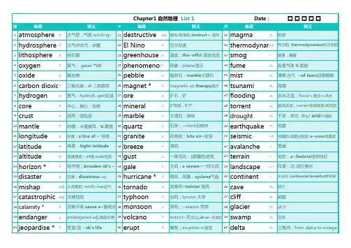
Chapter1 自然地理 List 1 Date: £££££1atmosphere n.大气层;气氛 working~21destructive adj.破坏/有害的 destruct v. 毁坏41magma n.岩浆adj.热力的, thermodynamics热力学的2hydrosphere n.大气中水汽,水圈22El Nino n.厄尔尼诺42thermodynamic3lithosphere n.岩石圈23greenhouse n.温室;the~effct 温室效应43smog n.烟雾,雾霾4oxygen n.氧气; gases 气体24phenomenon*n.现象;pheno显示44fume n.有害气体 V.冒烟5oxide n.氧化物25pebble n.鹅卵石;marble大理石45mist n.薄雾,水汽 ~of tears泪眼模糊6carbon dioxide n.二氧化碳;di 二的意思26magnet *n.magnetic adj therapy磁疗46tsunami n.海啸7hydrogen n.氢气;hydro水, gen生成27ore n.矿石,矿47flooding n.洪水泛滥;flood v.淹没 n.洪水8core n.中心,核心;地核28mineral n.矿物质;矿产48torrent n.激流洪流;current思潮趋势,现在的9crust n.地壳;面包皮29marble n.大理石;弹球49drought n.干旱,旱灾 dry/ arid干燥的10mantle n.地幔;斗篷披风;v.覆盖30quartz n.石英;~clock石英钟50earthquake n.地震11longitude n.经度;a line of ~ 经线31granite n.花岗岩;bite on~徒劳51seismic adj.地震的,地震引起的 a~wave地震波12latitude n.纬度;hight-latitude32breeze n.微风52avalanche n.雪崩13altitude n.高度海拔;alt高,itude性质33gust n.一阵狂风;(感情的)迸发53terrain n.地形;a~feature地形特征14horizon *n.地平线;broaden sb's ~34gale n.大风;a severe~一阵大风54landscape n/v风景;对..进行美化15disaster n.灾难;disastrous adj.35hurricane *n.飓风,风暴;cyclone气旋55continent n.大陆洲, continental breakfast欧早餐16mishap adj.小灾难的, mis坏+hap运气36tornado n.龙卷风=twister 旋风56cave n.洞穴17catastrophic adj.灾难性的37typhoon n.台风;tycoon 大亨57cliff n.峭壁18calamity *n.灾难不幸 cause a~酿成灾38monsoon n.季风;~season 雨季58glacier n.冰川19endanger v.endangered adj.濒临灭绝39volcano n.extinct~死火山,sit on~处境危险59swamp n.沼泽20jeopardise *v.危害/及 ~sb's life 40erupt v.爆发;eruption n.喷发60delta n.三角洲;from alpha to omega1plain n/adj平原;简单朴素的21pacific n/adj太平洋;平静的41steep adj.陡峭的,陡直的2plateau n.高原;~ climate高原气候22marine n/adj水兵;海洋的42parallel n/adj/v平行线;平行的;V.与...相似3oasis n.绿洲=water hole23navigation n.航行. navigator航海家/导航员43narrow n/adj/v窄/局限的.n海岸;V变窄; ~down限制减少4globe n.球体,地球仪24gulf n.海湾. golf高尔夫44Oceania n.大洋洲5hemisphere n.半球. hemispheric 半球的25beach n.海滩45mainland n.大陆本土=continent6equator n.赤道26coast n.海岸,海滨. coastal 海岸的46peninsula n.半岛7equal adj.相当的,all men are created~27shore n.(大水域的)岸47climate n.气候,思潮,环境8arctic n/adj北极的;the 北极地区28tide n.趋势/潮流.tidal的. at low~退潮时48weather n.天气,气象9Antarctic adj.南极的. ant对面+arctic29current n.水/气/电流. currently目前地49meteorology n.[miːtiəˈrɒlədʒi] 气象学.meteor高处物10pole n.两级中的一级30brook n.小河,溪50mild adj.温和的. a~climate温和气候11polar *adj.极地/对立的. polarize两极分化31stream n/v.小河,溪;V.流出51heating n.供暖.暖气,装置. heat热v.变热12axis n.轴线. axe斧头32source n.河源头, 根源. resource资源52moderate adj/v.适中的;缓和13deteriorate *v.恶化/严重.deterioration n.恶化33shallow adj.浅的. ~-hearted adj.薄情的53warm adj/v.暖和;变暖. warmth n.温暖热情14aggravate v.加重/恶化. gravity重力34superficial adj.表层的. a~injury 皮外伤54thermal adj.热量的;thermovent海底火山口15degrade *v.降解/贬低 degradeble可降解35flat adj/n.扁平的;公寓 55tropics adj/n.热带地区. tropical热带的; in the~ 16upgrade v.提高. ~(sth)to(sth)升级为36smooth adj.光滑/流畅的 smoothly adv.56arid adj.干燥的,干旱的. an~desert 干旱的荒漠17erode *v.侵蚀/腐蚀. erosion n.侵蚀37rough adj.粗糙的. roughly adv.57moist adj.潮湿的. moisture n潮湿,湿气,水分18Mediterranean adj.地中海的38sandy adj.含沙的,铺满沙. sand 沙/滩58damp adj.潮湿的. a~climate潮气候. dampness n. 19Atlantic n/adj大西洋;大西洋的39stony adj.石头的;多石的59humid adj.湿热的.~conditions. humidity n.高温潮20ocean n.海洋;~s of 大量的40vertical adj.垂直/直立的. 反:horizonal60snowy adj.下雪多的,被覆盖的1frost n.霜冻. frosty adj.严寒的21mount v/n.登上,渐渐增加;山41sediment n.沉积物2hail n/v.冰雹;赞扬,招呼,下冰雹22mountain n.山,高山42silt n/v.淤泥;堵塞3thaw v/n.解冻,融化~sth out;解冻时期23range n.山脉;范围. in the~of在..范围内43muddy adj.泥泞浑浊的. mud泥4chill v/n.使变冷;寒.~enthusiasm热情冷却24ridge n/v.山脉;使隆起44clay n.粘土,陶土5freeze v/n.结冰;霜冻. freezer冰柜25slope n/v.山坡,斜坡;倾斜45dirt n.污垢,灰尘泥土. dirty adj.脏的6frigid adj.寒冷的. a~climate极冷气候26valley n.山谷,溪谷. in the~在山谷里46rural adj.乡村的. ~area农村地区7tremble v/n.战抖. ~all over浑身颤抖27hillside n.山腰47suburb n.郊区. suburban adj.郊区的8shiver v.哆嗦. ~with cold冷得发抖28overlook *v.俯跳,忽视=neglect48outskirts n.郊区,市郊9thunder v/n.雷声,打雷. thunderstorm雷雨29southern adj.南方的49remote adj.遥远的. a~contorl 遥控器10lightning n/adj.闪电;闪电般快的. lighten v.变轻30southeast n/adj.东南方;东南方的50desolate adj.荒凉的11stormy adj.暴风雨的. storm n.暴风雨31southwest n/adj.西南方;西南方的51distant adj.疏远,遥远的. the~past遥远的过去12downpour n.倾盆大雨32northeast n/adj.东北部;东北部的52adjacent adj.邻近的. ~to与..临近13rainfall n.降雨量33northwest n/adj.西北部;西北部的53toxic adj.有毒的. highly~剧毒14sprinkle v/n.撒;少量,小雨. sprinker喷淋34eastern adj.东部的54pollution n.污染. pullute v.污染15rainbow n.彩虹35oriental *n.东方的(中国/日本) ~week新生周55pollutant n.污染物. atmosphere~大气污染物16shower n.阵雨;淋浴36inevitable adj.不可避免的. evitable可避免的56contaminate v.弄脏污染. con共同+tam触摸17Celsius adj/n.[ˈselsiəs]摄氏的;摄氏度 37irreversible adj.不可逆转的. ir不+re回+vers转57geology n.地质学;地质状况. geological adj. 18temperature n.气温,体温38irregularly adv.不规则. regularly规则地58border n/v.边界;和..毗邻. within the~of在..境内19forecast *v/n.预言/测;预报= foresee39inappropriate adj.不合适的. propre合适的59margin n.边缘,空白.allow a greater~of允许余地20peak n/v.山峰,顶点; 到最大值40abnormal adj.不正常的;变态 normal正常60fringe n/adj.边缘,刘海;次要的,非主流的Chapter1 自然地理 List 4 Date: £££££1plate n.地址板块,盘21sunset n.日落. ~glow晚霞.~industry夕阳产业41drown v.淹死,浸泡2debris n.残骸22eclipse n.日食月食. a solar/lunar~42blow v.风吹;用力一击. strikea~for维护3crack v/n.破裂/声;裂缝. cause a~弄裂痕23dusk n.黄昏. by~到黄昏时. 反:dawn破晓43puff v/n.喷出;吹出一缕4gap n.缺口,差距. the generation~代购24heaven n.天堂44gush v/n.涌出. ~out喷出. ~from从..喷出5splendid adj.极好/壮观的. a~chance25paradise n.天堂乐园45dense adj.密集的. density n.密度6grand adj.宏达的;豪华的26sunshine n.阳光46intensity n.强烈. intense adj.强烈的,紧张的7magnificent adj.壮丽的,令人印象深刻. magnificence27shade n/v.阴影;给..遮光. shady adj.阴凉的47intensive adj.加强/集中/密集的. intense剧烈的8super adj.超级的28shadow n.影子阴影. cast a~投下阴影48emerge v.浮现,暴漏. ~out of从..里出来9interesting adj.有趣的. interested adj. 感兴趣的29vapour n.vapor 蒸气,水汽49flash v/n.闪光闪现. ~through sb's mind 10dramatic adj.戏剧性的. a~event令人深刻事30evaporate v.蒸发,消失. evaporation n.50float v.漂浮11wilderness n.荒野31circulate v.循环,流通,传播. circulation n.51environment adj.环境. enviromental adj.有关环境的12desert n/v.沙漠;离弃.desertification荒漠化32precipitate v.凝结,沉淀. tion n.52surrounding adj.周围的. ~environment周围环境13deforest v.毁掉森林33reservoir n.水库. dam大坝53condition n.条件14barren adj.贫瘠的. a~desert荒漠34waterfall n.瀑布. firwork 烟花54situation n.情况. situate v.使位于15fertile adj.肥沃,富饶35fountain n.喷泉,源泉55nature n.自然,本质,性质.destroy~破坏自然16fertilise v.施肥. fertiliser n.肥料36spring n.春天,泉水. springtime 春季56natural adj.自然的. naturally adv.自然地17solar adj.太阳的37dew n.露水57artificial *adj.人造的18lunar adj.月亮的38pour v.倾斜,倾盆而下. downpour倾盆大雨58synthetic *adj.人造的,合成的19calendar n.历法,日历. lunar~阴历39drain v/n.排空;耗竭. drainage排水59petrol n.汽油. petroleum 石油20sunrise n.日出40drip v.滴出. drip down滴下60gas n.气体,汽油 gasoline汽油Chapter2 植物研究 List 6 Date: £££££1rainforest n.雨林. a~ reserve雨林保护区21meadow n.草地牧场41surroundings n.环境2jungle n.丛林22lawn n.草坪,草地42counterbalance n/v.平衡作用的事物;抵消,对...起作用3plantation n.种植园,栽植23olive n.橄榄树. an~brunch橄榄枝43mechanism v.机制,制造[ˈmekənɪzəm]4field n.田野,野外24pine n.松树,松木44preserve v.保护,维持原状,保存 v+ation n. 5terrace n.梯田25vine n.葡萄藤45conservation n.(对环境)保护. conversation交谈6timber n.木材26violet n.堇菜 [ˈvaɪələt]46bush fire n.林区大火7charcoal n.木炭27tulip n.郁金香 [ˈtjuːlɪp]47extinguish v.扑灭;破灭. extinguisher灭火器8log n.原木,航海日志28mint n/v.薄荷,铸币厂;造硬币48destruct v.自毁. destruction n.破坏9logo n.标示29reef n.暗礁. on the~49ruin v/n.毁坏;毁灭,废墟10forestry n.林学林业. forest 森林30alga n.海草. algal adj. algae复数50perish v.毁灭腐烂,消亡11branch n.树枝,分支分店31enzyme n.酶51demolish v.拆除毁坏,推翻12trunk n.树干,躯干;大箱子32catalyst n.催化剂,促成因素.catalyze v.52infringe v.违反;侵犯13bough n.大树枝33release n/v.释放发布53undermine v.破坏,逐渐消弱14root n/v.跟;生根34emission n.排放;排放物54extinction n.灭绝. extinc adj.已灭绝的15hay n.干草. hit the~ 上床睡觉35absorb v.吸收,吸引注意. be~in专注..上55pattern n.模式,底样16straw n.稻草,麦秆;吸管36circulation n.循环,流通. circle环绕 circulate流传56outcome n.结果17reed n.芦苇37exceed v.超过57impact n.影响18thorn n.刺,荆棘. thorny多刺棘手的38uptake n.摄取58seasonal adj.季节性的19weed n/v.杂草;除杂草39nutrient n.营养物. nutrition营养/学59experimental adj.实验的. vaccine疫苗20grass n.草地40energy n.能源,精力60favourable adj.有利的,赞成,肯定Chapter4 太空探索 List 10 Date: £££££1galaxy n.星系,银河系21propulsion n.推进力41fossil n.化石2cosmos n.宇宙22pressure n.压力42sample n.样品,样本3universe n.宇宙万物.universal adj.全世界的普遍的23dynamics n.动力学,动态. dynamic发动的43specimen n.样品,标本 species物种4interstellar adj.星际的。
IntroductiontoMarineBiogeochemistryTo adopt this book for course use, visit http://textbooks.elsevier.com Companion Web Site:http://elsevierdirect.com/companions/9780120885305
ELSEVIERscience &
technology books
Resources for Professors: •All figures from the book available in color (if applicable) as PowerPoint slides•Study guide and homework problems for students•Suggestions for supplemental readings, many of which are Web accessible•Two chapters and nine appendices available only on the Web•Full reference list
Introduction to Marine Biogeochemistry, Second Editionby Susan Libes
ACADEMICPRESS
TOOLSALLTEACHING
FORYOUR
NEEDS
textbooks.elsevier.comIntroductiontoMarineBiogeochemistry
SecondEdition
SusanLibesCollegeofNaturalandAppliedSciencesCoastalCarolinaUniversityConway,SouthCarolina
AMSTERDAM•BOSTON•HEIDELBERG•LONDONNEWYORK•OXFORD•PARIS•SANDIEGOSANFRANCISCO•SINGAPORE•SYDNEY•TOKYO
Chapter23Michelle Bodnar,Andrew LohrApril12,2016Exercise23.1-1Suppose that A is an empty set of edges.Then,make any cut that has(u,v) crossing it.Then,since that edge is of minimal weight,we have that(u,v)is a light edge of that cut,and so it is safe to add.Since we add it,then,once wefinish constructing the tree,we have that(u,v)is contained in a minimum spanning tree.Exercise23.1-2Let G be the graph with4vertices:u,v,w,z.Let the edges of the graph be (u,v),(u,w),(w,z)with weights3,1,and2respectively.Suppose A is the set {(u,w)}.Let S=A.Then S clearly respects A.Since G is a tree,its minimum spanning tree is itself,so A is trivially a subset of a minimum spanning tree. Moreover,every edge is safe.In particular,(u,v)is safe but not a light edge for the cut.Therefore Professor Sabatier’s conjecture is false.Exercise23.1-3Let T0and T1be the two trees that are obtained by removing edge(u,v) from a MST.Suppose that V0and V1are the vertices of T0and T1respectively. Consider the cut which separates V0from V1.Suppose to a contradiction that there is some edge that has weight less than that of(u,v)in this cut.Then,we could construct a minimum spanning tree of the whole graph by adding that edge to T1∪T0.This would result in a minimum spanning tree that has weight less than the original minimum spanning tree that contained(u,v).Exercise23.1-4Let G be a graph on3vertices,each connected to the other2by an edge, and such that each edge has weight1.Since every edge has the same weight, every edge is a light edge for a cut which it spans.However,if we take all edges we get a cycle.1Exercise23.1-5Let A be any cut that causes some vertices in the cycle on once side of the cut,and some vertices in the cycle on the other.For any of these cuts,we know that the edge e is not a light edge for this cut.Since all the other cuts wont have the edge e crossing it,we won’t have that the edge is light for any of those cuts either.This means that we have that e is not safe.Exercise23.1-6Suppose that for every cut of the graph there is a unique light edge crossing the cut,but that the graph has2spanning trees T and T .Since T and T are distinct,there must exist edges(u,v)and(x,y)such that(u,v)is in T but not T and(x,y)is in T but not T.Let S={u,x}.There is a unique light edge which spans this cut.Without loss of generality,suppose that it is not(u,v). Then we can replace(u,v)by this edge in T to obtain a spanning tree of strictly smaller weight,a contradiction.Thus the spanning tree is unique.For a counter example to the converse,let G=(V,E)where V={x,y,z} and E={(x,y),(y,z),(x,z)}with weights1,2,and1respectively.The unique minimum spanning tree consists of the two edges of weight1,however the cut where S={x}doesn’t have a unique light edge which crosses it,since both of them have weight1.Exercise23.1-7First,we show that the subset of edges of minimum total weight that con-nects all the vertices is a tree.To see this,suppose not,that it had a cycle. This would mean that removing any of the edges in this cycle would mean that the remaining edges would still connect all the vertices,but would have a total weight that’s less by the weight of the edge that was removed.This would con-tradict the minimality of the total weight of the subset of vertices.Since the subset of edges forms a tree,and has minimal total weight,it must also be a minimum spanning tree.To see that this conclusion is not true if we allow negative edge weights,we provide a construction.Consider the graph K3with all edge weights equal to −1.The only minimum weight set of edges that connects the graph has total weight−3,and consists of all the edges.This is clearly not a MST because it is not a tree,which can be easily seen because it has one more edge than a tree on three vertices should have.Any MST of this weighted graph must have weight that is at least-2.Exercise23.1-8Suppose that L is another sorted list of edge weights of a minimum span-ning tree.If L =L,there must be afirst edge(u,v)in T or T which is of smaller weight than the corresponding edge(x,y)in the other set.Without2loss of generality,assume(u,v)is in T.Let C be the graph obtained by adding (u,v)to L .Then we must have introduced a cycle.If there exists an edge on that cycle which is of larger weight than(u,v),we can remove it to obtain a tree C of weight strictly smaller than the weight of T ,contradicting the fact that T is a minimum spanning tree.Thus,every edge on the cycle must be of lesser or equal weight than(u,v).Suppose that every edge is of strictly smaller weight.Remove(u,v)from T to disconnect it into two components.There must exist some edge besides(u,v)on the cycle which would connect these,and since it has smaller weight we can use that edge instead to create a spanning tree with less weight than T,a contradiction.Thus,some edge on the cycle has the same weight as(u,v).Replace that edge by(u,v).The corresponding lists L and L remain unchanged since we have swapped out an edge of equal weight, but the number of edges which T and T have in common has increased by1. If we continue in this way,eventually they must have every edge in common, contradicting the fact that their edge weights differ somewhere.Therefore all minimum spanning trees have the same sorted list of edge weights.Exercise23.1-9Suppose that there was some cheaper spanning tree than T .That is,we have that there is some T so that w(T )<w(T ).Then,let S be the edges in T but not in T .We can then construct a minimum spanning tree of G by considering S∪T .This is a spanning tree since S∪T is,and T makes all the vertices in V connected just like T does.However,we have that w(S∪T )=w(S)+w(T )<w(S)+w(T )=w(S∪T )=w(T).This means that we just found a spanning tree that has a lower total weight than a minimum spanning tree.This is a contradiction,and so our assumption that there was a spanning tree of V cheaper than T must be false.Exercise23.1-10Suppose that T is no longer a minimum spanning tree for G with edge weights given by w .Let T be a minimum spanning tree for this graph.Then we have we have w (T )<w(T)−k.Since the edge(x,y)may or may not be in T we have w(T )≤w (T )+k<w(T),contradicting the fact that T was minimal under the weight function w.Exercise23.1-11If we were to add in this newly decreased edge to the given tree,we would be creating a cycle.Then,if we were to remove any one of the edges along this cycle,we would still have a spanning tree.This means that we look at all the weights along this cycle formed by adding in the decreased edge,and remove the edge in the cycle of maximum weight.This does exactly what we want since we could only possibly want to add in the single decreased edge,and then,from there we change the graph back to a tree in the way that makes its total weight3minimized.Exercise23.2-1Suppose that we wanted to pick T as our minimum spanning tree.Then,to obtain this tree with Kruskal’s algorithm,we will order the edgesfirst by their weight,but then will resolve ties in edge weights by picking an edgefirst if it is contained in the minimum spanning tree,and treating all the edges that aren’t in T as being slightly larger,even though they have the same actual weight. With this ordering,we will still befinding a tree of the same weight as all the minimum spanning trees w(T).However,since we prioritize the edges in T,we have that we will pick them over any other edges that may be in other minimum spanning trees.Exercise23.2-2At each step of the algorithm we will add an edge from a vertex in the tree created so far to a vertex not in the tree,such that this edge has minimum weight.Thus,it will be useful to know,for each vertex not in the tree,the edge from that vertex to some vertex in the tree of minimal weight.We will store this information in an array A,where A[u]=(v,w)if w is the weight of(u,v) and is minimal among the weights of edges from u to some vertex v in the tree built so far.We’ll use A[u].1to access v and A[u].2to access w.Algorithm1PRIM-ADJ(G,w,r)Initialize A so that every entry is(NIL,∞)T={r}for i=1to V doif Adj[r,i]=0thenA[i]=(r,w(r,i))end ifend forfor each u∈V−T dok=min i A[i].2T=T∪{k}k.π=A[k].1for i=1to V doif Adj[k,i]=0and Adj[k,i]<A[i].2thenA[i]=(k,Adj[k,i])end ifend forend forExercise23.2-34Prim’s algorithm implemented with a Binary heap has runtime O((V+ E)lg(V)),which in the sparse case,is just O(V lg(V)).The implementation with Fibonacci heaps is O(E+V lg(V))=O(V+V lg(V))=O(V lg(V)).So, in the sparse case,the two algorithms have the same asymptotic runtimes.In the dense case,we have that the binary heap implementation has runtime O((V+E)lg(V))=O((V+V2)lg(V))=O(V2lg(V)).The Fibonacci heap implementation however has a runtime of O(E+V lg(V))=O(V2+V lg(V))= O(V2).So,in the dense case,we have that the Fibonacci heap implementation is asymptotically faster.The Fibonacci heap implementation will be asymptotically faster so long as E=ω(V).Suppose that we have some function that grows more quickly than linear,say f,and E=f(V).The binary heap implementation will have runtime O((V+E)lg(V))=O((V+f(V))lg(V))=O(f(V)lg(V)).However, we have that the runtime of the Fibonacci heap implementation will have run-time O(E+V lg(V))=O(f(V)+V lg(V)).This runtime is either O(f(V))or O(V lg(V))depending on if f(V)grows more or less quickly than V lg(V)re-spectively.In either case,we have that the runtime is faster than O(f(V)lg(V)).Exercise23.2-4If the edge weights are integers in the range from1to|V|,we can make Kruskal’s algorithm run in O(Eα(V))time by using counting sort to sort the edges by weight in linear time.I would take the same approach if the edge weights were integers bounded by a constant,since the runtime is dominated by the task of deciding whether an edge joins disjoint forests,which is independent of edge weights.Exercise23.2-5If there the edge weights are all in the range1,...,|V|,then,we can imagine adding the edges to an array of lists,where the edges of weight i go into the list in index i in the array.Then,to decrease an element,we just remove it from the list currently containing it(constant time)and add it to the list corresponding to its new value(also constant time).To extract the minimum wight edge,we maintain a linked list among all the indices that contain non-empty lists,which can also be maintained with only a constant amount of extra work.Since all of these operations can be done in constant time,we have a total runtime O(E+V).If the edge weights all lie in some bounded universe,suppose in the range 1to W.Then,we can just vEB tree structure given in chapter20to have the two required operations performed in time O(lg(lg(W))),which means that the total runtime could be made O((V+E)lg(lg(W))).Exercise23.2-6For input drawn from a uniform distribution I would use bucket sort with5Kruskal’s algorithm,for expected linear time sorting of edges by weight.This would achieve expected runtime O(Eα(V)).Exercise23.2-7Wefirst add all the edges to the new vertex.Then,we preform a DFS rooted at that vertex.As we go down,we keep track of the largest weight edge seen so far since each vertex above us in the DFS.We know from exercise23.3-6that in a directed graph,we don’t need to consider cross or forward edges.Every cycle that we detect will then be formed by a back edge.So,we just remove the edge of greatest weight seen since we were at the vertex that the back edge is going to.Then,we’ll keep going until we’ve removed one less than the degree of the vertex we added many edges.This will end up being linear time since we can reuse part of the DFS that we had already computed before detecting each cycle.Exercise23.2-8Professor Borden is mistaken.Consider the graph with4vertices:a,b,c, and d.Let the edges be(a,b),(b,c),(c,d),(d,a)with weights1,5,1,and5 respectively.Let V1={a,d}and V2={b,c}.Then there is only one edge incident on each of these,so the trees we must take on V1and V2consist of precisely the edges(a,d)and(b,c),for a total weight of10.With the addition of the weight1edge that connects them,we get weight11.However,an MST would use the two weight1edges and only one of the weight5edges,for a total weight of7.Problem23-1a.To see that the second best minimum spanning tree need not be unique,weconsider the following example graph on four vertices.Suppose the vertices are{a,b,c,d},and the edge weights are as follows:a b c da−143b1−52c45−6d326−Then,the minimum spanning tree has weight7,but there are two spanning trees of the second best weight,8.b.We are trying to show that there is a single edge swap that can demote ourminimum spanning tree to a second best minimum spanning tree.In obtaining the second best minimum spanning tree,there must be some cut of a single vertex away from the rest for which the edge that is added is not light,otherwise,we wouldfind the minimum spanning tree,not the second best minimum spanning tree.Call the edge that is selected for that cut for6the second best minimum spanning tree(x,y).Now,consider the same cut, except look at the edge that was selected when obtaining T,call it(u,v).Then,we have that if consider T−{(u,v)}∪{(x,y)},it will be a second best minimum spanning tree.This is because if the second best minimum spanning tree also selected a non-light edge for another cut,it would end up more expensive than all the minimum spanning trees.This means that we need for every cut other than the one that the selected edge was light.This means that the choices all align with what the minimum spanning tree was.c.We give here a dynamic programming solution.Suppose that we want tofind it for(u,v).First,we will identify the vertex x that occurs immediately after u on the simple path from u to v.We will then make max[u,v]equal to the max of w((u,x))and max[w,v].Lastly,we just consider the case that u and v are adjacent,in which case the maximum weight edge is just the single edge between the two.If we canfind x in constant time,then we will have the whole dynamic program running in time O(V2),since that’s the size of the table that’s being built up.Tofind x in constant time,we preprocess the tree.Wefirst pick an arbitrary root.Then,we do the preprocessing for Tarjan’s off-line least common an-cestors algorithm(See problem21-3).This takes time just a little more than linear,O(|V|α(|V|)).Once we’ve computed all the least common ancestors, we can just look up that result at some point later in constant time.Then, tofind the w that we should pick,wefirst see if u=LCA(u,v)if it does not,then we just pick the parent of u in the tree.If it does,then weflip the question on its head and try to compute max[v,u],we are guaranteed to not have this situation of v=LCA(v,u)because we know that u is an ancestor of v.d.We provide here an algorithm that takes time O(V2)and leave open if thereexists a linear time solution,that is a O(E+V)time solution.First,we find a minimum spanning tree in time O(E+V lg(V)),which is in O(V2).Then,using the algorithm from part c,wefind the double array max.Then, we take a running minimum over all pairs of vertices u,v,of the value of w(u,v)−max[u,v].If there is no edge between u and v,we think of the weight being infinite.Then,for the pair that resulted in the minimum value of this difference,we add in that edge and remove from the minimum spanning tree, an edge that is in the path from u to v that has weight max[u,v].Problem23-2a.We’ll show that the edges added at each step are safe.Consider an un-marked vertex u.Set S={u}and let A be the set of edges in the tree so far. Then the cut respects A,and the next edge we add is a light edge,so it is safe for A.Thus,every edge in T before we run Prim’s algorithm is safe for T.Any edge that Prim’s would normally add at this point would have to connect two7of the trees already created,and it would be chosen as minimal.Moreover,we choose exactly one between any two trees.Thus,the fact that we only have the smallest edges available to us is not a problem.The resulting tree must be minimal.b.We argue by induction on the number of vertices in G.We’ll assume that|V|>1,since otherwise MST-REDUCE will encounter an error on line6 because there is no way to choose v.Let|V|=2.Since G is connected,there must be an edge between u and v,and it is trivially of minimum weight.They are joined,and|G .V|=1=|V|/2.Suppose the claim holds for|V|=n.Let G be a connected graph on n+1vertices.Then G .V≤n/2prior to thefinal vertex v being examined in the for-loop of line4.If v is marked then we’re done, and if v isn’t marked then we’ll connect it to some other vertex,which must be marked since v is the last to be processed.Either way,v can’t contribute an additional vertex to G .V,so|G .V|≤n/2≤(n+1)/2.c.Rather than using the disjoint set structures of chapter21,we can simply use an array to keep track of which component a vertex is in.Let A be an array of length|V|such that A[u]=v if v=F IND−SET(u).Then FIND-SET(u) can now be replaced with A[u]and UNION(u,v)can be replaced by A[v]=A[u]. Since these operations run in constant time,the runtime is O(E).d.The number of edges in the output is monotonically decreasing,so each call is O(E).Thus,k calls take O(kE)time.e.The runtime of Prim’s algorithm is O(E+V lg V).Each time we run MST-REDUCE,we cut the number of vertices at least in half.Thus,af-ter k calls,the number of vertices is at most|V|/2k.We need to minimizeE+V/2k lg(V/2k)+kE=E+V lg(V)k −V kk+kE with respect to k.If we choosek=lg lg V then we achieve the overall running time of O(E lg lg V)as desired.To see that this value of k minimizes,note that the V k2k term is always less thanthe kE term since E≥V.As k decreases,the contribution of kE decreases,and the contribution of V lg V2k increases.Thus,we need tofind the value of kwhich makes them approximately equal in the worst case,when E=V.Todo this,we set lg V2k =k.Solving this exactly would involve the Lambert Wfunction,but the nicest elementary function which gets close is k=lg lg V.f.We simply set up the inequality E lg lg V<E+V lg V tofind that weneed E<V lg Vlg lg V−1=OV lg Vlg lg V.Problem23-3a.To see that every minimum spanning tree is also a bottleneck spanning tree.Suppose that T is a minimum spanning tree.Suppose there is some edge in it(u,v)that has a weight that’s greater than the weight of the bottleneck8spanning tree.Then,let V1be the subset of vertices of V that are reach-able from u in T,without going though v.Define V2symmetrically.Then, consider the cut that separates V1from V2.The only edge that we could add across this cut is the one of minimum weight,so we know that there are no edge across this cut of weight less than w(u,v).However,we have that there is a bottleneck spanning tree with less than that weight.This is a contradiction because a bottleneck spanning tree,since it is a spanning tree, must have an edge across this cut.b.To do this,wefirst process the entire graph,and remove any edges thathave weight greater than b.If the remaining graph is selected,we can just arbitrarily select any tree in it,and it will be a bottleneck spanning tree of weight at most b.Testing connectivity of a graph can be done in linear time by running a breadthfirst search and then making sure that no vertices remain white at the end.c.Write down all of the edge weights of e the algorithm from section9.3tofind the median of this list of numbers in time O(E).Then,run theprocedure from part b with this median value as the one that you are testing for there to be a bottleneck spanning tree with weight at most.Then there are two cases:First,we could have that there is a bottleneck spanning tree with weight at most this median.Then just throw the edges with weight more than the median,and repeat the procedure on this new graph with half the edges.Second,we could have that there is no bottleneck spanning tree with at most that weight.Then,we should run the procedure from problem23-2 to contract all of the edges that have weight at most this median weight.This takes time O(E lg(lg(V)))and then we are left solving the problem ona graph that now has half the vertices.Problem23-4a.This does return an MST.To see this,we’ll show that we never remove anedge which must be part of a minimum spanning tree.If we remove e,thene cannot be a bridge,which means that e lies on a simple cycle of the graph.Since we remove edges in nonincreasing order,the weight of every edge on the cycle must be less than or equal to that of e.By exercise23.1-5,there isa minimum spanning tree on G with edge e removed.To implement this,we begin by sorting the edges in O(E lg E)time.For each edge we need to check whether or not T−{e}is connected,so we’ll need to run a DFS.Each one takes O(V+E),so doing this for all edges takes O(E(V+E).This dominates the running time,so the total time is O(E2).9b.This doesn’t return an MST.To see this,let G be the graph on3verticesa,b,and c.Let the eges be(a,b),(b,c),and(c,a)with weights3,2,and1 respectively.If the algorithm examines the edges in their order listed,it will take the two heaviest edges instead of the two lightest.An efficient implementation will use disjoint sets to keep track of connected components,as in MST-REDUCE in problem23-2.Trying to union within the same component will create a cycle.Since we make|V|calls to MAKE-SET and at most3|E|calls to FIND-SET and UNION,the runtime is O(Eα(V)).c.This does return an MST.To see this,we simply quote the result from exer-cise23.1-5.The only edges we remove are the edges of maximum weight on some cycle,and there always exists a minimum spanning tree which doesn’t include these edges.Moreover,if we remove an edge from every cycle then the resulting graph cannot have any cycles,so it must be a tree.To implement this,we use the approach taken in part(b),except now we also need tofind the maximum weight edge on a cycle.For each edge which introduces a cycle we can perform a DFS tofind the cycle and max weight edge.Since the tree at that time has at most one cycle,it has at most|V| edges,so we can run DFS in O(V).The runtime is thus O(EV).10。
Part ThreeChapter 23 Canada‟s geography and history加拿大的地理特点:Canada’s geography features:1) 座落于美国的北部,仅次于俄罗斯的世界第二大国;lies to the north of the US; the world‟s second largest country after Russia.2.地形十分复杂:东部山区沿海省份沿劳伦斯湾和大西洋形成不规则的海岸;西部,太平洋沿岸地区被南北走向的山脉分离,其中包括落基山脉;中部是一个大平原;it has an extremely varied topography:the east part is mountainous maritime provinces have an irregular coastline on the Gulf of St. Lawrence and the Atlantic;The west part,the Pacific border is separated from the rest of the country by mountain ranges from north to south including the Rockies; the central part is a vast plain.3.气候不甚宜人,大部分地区冬季既漫长又寒冷,积雪深厚;所以,大多数人都居住在南部边境地区the climate is unfavorable, much of Canada has long and cold winters with deep snow. So,a major part of the population lives along the southern border.4.最高峰是落根峰,主要的两大河流是马更些河与圣劳伦斯河。
Chapter 23: Using the Eulerian Multiphase Model for Granular FlowThis tutorial is divided into the following sections:23.1. Introduction23.2. Prerequisites23.3. Problem Description23.4. Setup and Solution23.5. Summary23.6. Further Improvements
23.1. Introduction
Mixing tanks are used to maintain solid particles or droplets of heavy fluids in suspension. Mixing maybe required to enhance reaction during chemical processing or to prevent sedimentation. In this tutorial,you will use the Eulerian multiphase model to solve the particle suspension problem.The Eulerianmultiphase model solves momentum equations for each of the phases, which are allowed to mix in anyproportion.
This tutorial demonstrates how to do the following:•Use the granular Eulerian multiphase model.•Specify fixed velocities with a user-defined function (UDF) to simulate an impeller.•Set boundary conditions for internal flow.•Calculate a solution using the pressure-based solver.•Solve a time-accurate transient problem.