matlab计量经济学工具箱

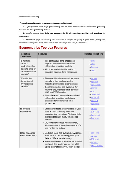
Econometric ModelingA simple model is easier to estimate, forecast, and interpret.1．Specification tests helps you identify one or more model families that could plausibly describe the data generating process.2．Model comparisons help you compare the fit of competing models, with penalties for complexity.3．Goodness-of-fit checks help you assess the in-sample adequacy of your model, verify that all model assumptions hold, and evaluate out-of-sample forecast performance.arimagarchegarchgjr(s a variant of the GARCH conditional variance model, named for Glosten, Jagannathan, and Runkle)A model object holds all the information necessary to estimate, simulate, and forecast econometric models.Parametric form of the modelNumber of model parameters (e.g., the degree of the model)Innovation distribution (Gaussian or Student's t)Amount of presample data needed to initialize the modelExample1: AR(2)where the innovations are independent and identically distributed normal random variables with mean 0 and variance 0.2. This is a conditional mean model, so use arima.>>model = arima('AR',{0.8,-0.2},'Variance',0.2,'Constant',0)Example2: GARCH(1,1) model>>model = garch('GARCH',NaN,'ARCH',NaN)或者>>model = garch(1,1)Parameters with NaN values need to be estimated or otherwise specified before you can forecast or simulate the model.To display the value of the property AR for the created variable object，>>model.AR>>model.Distribution = struct('Name','t','DoF',8)Methods are functions that accept model objects as inputs. In Econometrics Toolbox,estimateinferforecastsimulateExample3: Fit an ARMA(2,1) model to simulated data1) Simulate 500 data points from the ARMA(2,1) model>>simModel = arima('AR',{0.5,-0.3},'MA',0.2,'Constant',0,'Variance',0.1);>>rng(5);>>Y = simulate(simModel,500);2) Specify an ARMA(2,1) model with no constant and unknown coefficients and variance.>>model = arima(2,0,1);>>model.Constant = 03) Fit the ARMA(2,1) model to Y.>>fit = estimate(model,Y)Example4: infer>>load Data_EquityIdx>>nasdaq = Dataset.NASDAQ;>>r = price2ret(nasdaq);>>r0 = r(1:2);>>rn = r(3:end);Fit a GARCH(1,1) model to the returns, and infer the loglikelihood objective function value.>>model1 = garch(1,1);>>fit1 = estimate(model1,rn,'E0',r0);>>[~,LogL1] = infer(fit1,rn,'E0',r0);Wold's theorem: you can write all weakly stationary stochastic processes in the general linear form,Thus, by Wold's theorem, you can model(or closely approximate) every stationary stochastic process asThe conditional mean and variance modelsStationarity tests If your data is not stationary, consider transforming your data. Stationarity is the foundation of many time series models.You can difference a series with a unit root until it is stationary, Or, consider using a nonstationary ARIMA model if there is evidence of a unit root in your data.Seasonal ARIMA models use seasonal differencing to remove seasonal effects. You can also include seasonal lags to model seasonal autocorrelation.Conduct a Ljung-Box Q-test to test autocorrelations at several lags jointly. If autocorrelation is present, consider using a conditional mean model.Looking for autocorrelation in the squared residual series is one way to detect conditional Heteroscedasticity. To model conditional heteroscedasticity, consider using a conditional variance model.You can use a Student’s t distribution to model fatter tails than a Gaussian distribution (excess kurtosis).You can compare nested models using misspecification tests, such as the likelihood ratio test, Wald’s test, or Lagrange multiplier test.The Johansen and Engle-Granger cointegration tests assess evidence of cointegration. Consider using the VEC model for modeling multivariate, cointegrated series. It can introduce spurious regression effects.The example “Specifying Static Time Series Models” explores cointegration in static regression models. Type >> showdemo Demo_StaticModels.Why Transform?Isolate temporal components of interest.Remove the effect of nuisance components (like seasonality). Make a series stationary.Reduce spurious regression effects.Stabilize variability that grows with the level of the series.Make two or more time series more directly comparable.P207An example of a static conditional mean model is the ordinary linear regression model.Examples:By Wold’s decomposition, you can write the conditional mean of any stationary process y t asAnd is the constant unconditional mean of the stationary process.arima(p,D,q): nonseasonal AR terms (p), the order of nonseasonal integration (D), and the number of nonseasonal MA terms (q).When simulating time series models, one draw (or, realization) is an entire sample path of specified length N, y1, y2,...,y N, generate M sample paths, each of length N.Some extensions of Monte Carlo simulation rely on generating dependent random draws, such as Markov Chain Monte Carlo (MCMC). The simulate method in Econometrics Toolbox generates independent realizations.•Demonstrating theoretical results•Forecasting future events•Estimating the probability of future events1)Specifying any required presample data (or use default presample data).2)Generating an uncorrelated innovation series from the specified innovation distribution.3)Generating responses by recursively applying the specified AR and MA polynomial operators.The AR polynomial operator can include differencing.• Fo r stationary processes, presample responses are set to the unconditional mean of the process. • For nonstationary processes, presample responses are set to zero.• Presample innovations are set to zero.Step 1. Specify a model.>>model = arima('Constant',0.5,'AR',{0.7,0.25},'Variance',.1);Step 2. Generate one sample path.>>rng('default')>>Y = simulate(model,50);>>figure(1)>>plot(Y)>>xlim([0,50])>>title('Simulated AR(2) Process')Step 3. Generate many sample paths.rng('default')Y = simulate(model,50,'numPaths',1000);figure(2)subplot(2,1,1)plot(Y,'Color',[.85,.85,.85])title('Simulated AR(2) Process')hold onh=plot(mean(Y,2),'k','LineWidth',2);legend(h,'Simulation Mean','Location','NorthWest')hold offsubplot(2,1,2)plot(var(Y,0,2),'r','LineWidth',2)title('Process Variance')hold onplot(1:50,.83*ones(50,1),'k--','LineWidth',1.5)legend('Simulation','Theoretical',...'Location','SouthEast')hold offStep 4. Oversample the process.To reduce transient effects, one option is to oversample the process, simulate paths of length 150, and discard the first 100 observations.Step 1. Generate realizations from a trend-stationary process.t = [1:200]';trend = 0.5*t;model = arima('Constant',0,'MA',{1.4,0.8},'Variance',8);rng('default')u = simulate(model,300,'numPaths',50);Yt = repmat(trend,1,50) + u(101:300,:);Step 2. Generate realizations from a difference-stationary process.>>model = arima('Constant',0.5,'D',1,'MA',{1.4,0.8},'Variance',8);•V olatility clustering. V olatility is the conditional standard deviation of a time series. Autocorrelation in the conditional variance process results in volatility clustering.• Leverage effects. The volatility of some time series responds more to large decreases than to large increases. The EGARCH and GJR models have leverage terms to model this asymmetry.GARCH ModelEGARCH ModelStep 1. Load the data.Load the exchange rate data included with the toolbox.load Data_MarkPoundY = Data;N = length(Y);figure(1)plot(Y)set(gca,'XTick',[1,659,1318,1975]);set(gca,'XTickLabel',{'Jan 1984','Jan 1986','Jan 1988',...'Jan 1992'})ylabel('Exchange Rate')title('Deutschmark/British Pound Foreign Exchange Rate')Step 2. Calculate the returns.Convert the series to returns. This results in the loss of the first observation. r = price2ret(Y);figure(2)plot(2:N,r)set(gca,'XTick',[1,659,1318,1975]);set(gca,'XTickLabel',{'Jan 1984','Jan 1986','Jan 1988',...'Jan 1992'})ylabel('Returns')title('Deutschmark/British Pound Daily Returns')Step 3. Check for autocorrelation.Check the returns series for autocorrelation. Plot the sample ACF and PACF, and conduct a Ljung-Box Q-test.figure(3)subplot(2,1,1)autocorr(r)subplot(2,1,2)parcorr(r)[h,p] = lbqtest(r,[5 10 15])Step 4. Check for conditional heteroscedasticity.figure(4)subplot(2,1,1)autocorr((r-mean(r)).^2)subplot(2,1,2)parcorr((r-mean(r)).^2)[h,p] = archtest(r-mean(r),'lags',2)Step 5. Specify a GARCH(1,1) model.model = garch('Offset',NaN,'GARCHLags',1,'ARCHLags',1)Step 1. Load the data.Load the Danish nominal stock return data included with the toolbox.load Data_DanishY = Dataset.RN;N = length(Y);figure(1)plot(Y)xlim([0,N])title('Danish Nominal Stock Returns')Step 2. Fit an EGARCH(1,1) model.Specify, and then fit an EGARCH(1,1) model to the nominal stock returns series. Include a mean offset, and assume a Gaussian innovation distribution. model = egarch('Offset',NaN','GARCHLags',1,...'ARCHLags',1,'LeverageLags',1);fit = estimate(model,Y);Step 3. Infer the conditional variances.Infer the conditional variances using the fitted model.V = infer(fit,Y);figure(2)plot(V)xlim([0,N])title('Inferred Conditional Variances')Step 4. Compute the standardized residuals.Compute the standardized residuals for the model fit. Subtract the estimated mean offset, and divide by the square root of the conditional variance process. res = (Y-fit.Offset)./sqrt(V);figure(3)subplot(2,2,1)plot(res)xlim([0,N])title('Standardized Residuals') subplot(2,2,2)hist(res)subplot(2,2,3)autocorr(res)subplot(2,2,4)parcorr(res)Resampling StatisticsBootstrap JackknifeThe bootstrap procedure：each observation is selected separately at random from the original dataset.>>load lawdata>>plot(lsat,gpa,'+')>>lsline>>rhohat = corr(lsat,gpa)though it may seem large, you still do not know if it is statistically significant.Using the bootstrp function you can resample the lsat and gpa vectors as many times as you like and consider the variation in the resulting correlation coefficients.>>rhos1000 = bootstrp(1000,'corr',lsat,gpa);This command resamples the lsat and gpa vectors 1000 times and computes the corr function on each sample.>>hist(rhos1000,30)>>set(get(gca,'Children'),'FaceColor',[.8 .8 1])Nearly all the estimates lie on the interval [0.4 1.0].>>ci = bootci(5000,@corr,lsat,gpa)to obtain a confidence interval under 95% .The jackknife computes sample statistics on n separate samples of size n-1, Each sample is the original data with a single observation omitted.You can use the jackknife to estimate the bias, which is the tendency of the sample correlation to over-estimate or under-estimate the true, unknown correlation.>>jackrho = jackknife(@corr,lsat,gpa);>>meanrho = mean(jackrho)>>n = length(lsat);>>biasrho = (n-1) * (meanrho-rhohat)biasrho = -0.0065The sample correlation probably underestimates the true correlation by about this amount.。

Ｔoolbox工具箱序号工具箱备注一、数学、统计与优化1Symbolic Math Toolbox符号数学工具箱Symbolic Math Toolbox™提供用于求解和推演符号运算表达式以及执行可变精度算术的函数。

您可以通过分析执行微分、积分、化简、转换以及方程求解。

另外，还可以利用符号运算表达式为MATLAB®、Simulink®和Simscape™生成代码。

Symbolic Math Toolbox 包含MuPAD®语言，并已针对符号运算表达式的处理和执行进行优化。

该工具箱备有MuPAD 函数库，其中包括普通数学领域的微积分和线性代数，以及专业领域的数论和组合论。

此外，还可以使用MuPAD 语言编写自定义的符号函数和符号库。

MuPAD 记事本支持使用嵌入式文本、图形和数学排版格式来记录符号运算推导。

您可以采用HTML 或PDF 的格式分享带注释的推导。

2Partial Differential Euqation Toolbox偏微分方程工具箱偏微分方程工具箱™提供了用于在2D，3D求解偏微分方程（PDE）以及一次使用有限元分析。

它可以让你指定和网格二维和三维几何形状和制定边界条件和公式。

你能解决静态，时域，频域和特征值问题在几何领域。

功能进行后处理和绘图效果使您能够直观地探索解决方案。

你可以用偏微分方程工具箱，以解决从标准问题，如扩散，传热学，结构力学，静电，静磁学，和AC电源电磁学，以及自定义，偏微分方程的耦合系统偏微分方程。

3Statistics Toolbox统计学工具箱分类算法用于依据数据执行推理并构建预测模型。

4Curve Fitting Toolbox曲线拟合工具箱Curve Fitting Toolbox™提供了用于拟合曲线和曲面数据的应用程序和函数。

使用该工具箱可以执行探索性数据分析，预处理和后处理数据，比较候选模型，删除偏值。

您可以使用随带的线性和非线性模型库进行回归分析，也可以指定您自行定义的方程式。

6.1.1MA TLAB中常用的工具箱MA TLAB中常用的工具箱有：Matlab main toolbox——matlab主工具箱Control system toolbox——控制系统工具箱Communication toolbox——通信工具箱Financial toolbox——财政金融工具箱System identification toolbox——系统辨识工具箱Fuzzy logic toolbox ——模糊逻辑工具箱Higher-order spectral analysis toolbox——高阶谱分析工具箱Image processing toolbox——图像处理工具箱Lmi contral toolbox——线性矩阵不等式工具箱Model predictive contral toolbox——模型预测控制工具箱U-Analysis ang sysnthesis toolbox——u分析工具箱Neural network toolbox——神经网络工具箱Optimization toolbox——优化工具箱Partial differential toolbox——偏微分奉承工具箱Robust contral toolbox——鲁棒控制工具箱Spline toolbox——样条工具箱Signal processing toolbox——信号处理工具箱Statisticst toolbox——符号数学工具箱Symulink toolbox——动态仿真工具箱System identification toolbox——系统辨识工具箱Wavele toolbox——小波工具箱6.2优化工具箱中的函数1、最小化函数2、最小二乘问题3、方程求解函数4、演示函数中型问题方法演示函数大型文体方法演示函数。

MATLAB常用工具箱与函数库介绍1. 统计与机器学习工具箱（Statistics and Machine Learning Toolbox）：该工具箱提供了各种统计分析和机器学习算法的函数，包括描述统计、概率分布、假设检验、回归分析、分类与聚类等。

可以用于进行数据探索和建模分析。

2. 信号处理工具箱（Signal Processing Toolbox）：该工具箱提供了一系列信号处理的函数和算法，包括滤波、谱分析、信号生成与重构、时频分析等。

可以用于音频处理、图像处理、通信系统设计等领域。

3. 控制系统工具箱（Control System Toolbox）：该工具箱提供了控制系统设计与分析的函数和算法，包括系统建模、根轨迹设计、频域分析、状态空间分析等。

可以用于控制系统的设计和仿真。

4. 优化工具箱（Optimization Toolbox）：该工具箱提供了各种数学优化算法，包括线性规划、非线性规划、整数规划、最优化等。

可以用于寻找最优解或最优化问题。

5. 图像处理工具箱（Image Processing Toolbox）：该工具箱提供了图像处理和分析的函数和算法，包括图像滤波、边缘检测、图像分割、图像拼接等。

可以用于计算机视觉、医学影像处理等领域。

6. 神经网络工具箱（Neural Network Toolbox）：该工具箱提供了神经网络的建模和训练工具，包括感知机、多层前馈神经网络、循环神经网络等。

可以用于模式识别、数据挖掘等领域。

7. 控制系统设计工具箱（Robust Control Toolbox）：该工具箱提供了鲁棒控制系统设计与分析的函数和算法，可以处理不确定性和干扰的控制系统设计问题。

8. 信号系统工具箱（Signal Systems Toolbox）：该工具箱提供了分析、设计和模拟线性时不变系统的函数和算法。

可以用于信号处理、通信系统设计等领域。

9. 符号计算工具箱（Symbolic Math Toolbox）：该工具箱提供了符号计算的功能，可以进行符号表达式的运算、求解方程、求解微分方程等。

MATLAB常用工具箱与函数库介绍1. 引言MATLAB是一款功能强大的数学软件，广泛应用于工程、科学、计算机科学等领域。

在MATLAB中，有许多常用的工具箱和函数库，可以帮助用户解决各种数学计算和数据处理问题。

本文将介绍几个常用的MATLAB工具箱和函数库，帮助读者更好地理解和使用这些工具。

2. 统计工具箱统计工具箱是MATLAB中一个重要的工具箱，用于统计数据的分析和处理。

这个工具箱提供了许多函数，如直方图、概率分布函数、假设检验等等。

读者可以使用统计工具箱来分析数据的分布特征、计算数据的均值和标准差、进行假设检验等。

3. 信号处理工具箱信号处理工具箱是MATLAB中用于处理信号的一个重要工具箱。

它提供了一些常用的函数，如滤波器、谱分析、窗函数等等。

利用信号处理工具箱，读者可以对信号进行滤波、频谱分析、窗函数设计等操作，帮助解决各种与信号处理相关的问题。

4. 优化工具箱优化工具箱是MATLAB中用于求解优化问题的一个重要工具箱。

它提供了一些常用的函数，如线性规划、非线性规划、整数规划等等。

利用优化工具箱，读者可以求解各种优化问题，如优化算法选择、变量约束等。

优化工具箱在生产、物流、金融等领域具有广泛的应用。

5. 控制系统工具箱控制系统工具箱是MATLAB中一个针对控制系统设计和分析的重要工具箱。

它提供了一些常用的函数，如系统模型构建、控制器设计、系统分析等。

利用控制系统工具箱，读者可以构建控制系统模型、设计控制器、进行系统稳定性分析等操作。

这个工具箱在自动化控制领域非常有用。

6. 图像处理工具箱图像处理工具箱是MATLAB中一个用于处理和分析图像的重要工具箱。

它提供了一些常用的函数，如图像滤波、边缘检测、图像分割等等。

利用图像处理工具箱，读者可以对图像进行滤波、边缘检测、目标分割等操作，帮助解决图像处理中的各种问题。

7. 符号计算工具箱符号计算工具箱是MATLAB中一个用于进行符号计算的重要工具箱。

MATLAB工具箱的功能及使用方法引言：MATLAB是一种常用的用于数值计算和科学工程计算的高级计算机语言和环境。

它的灵活性和强大的计算能力使得它成为工程师、科学家和研究人员的首选工具之一。

而在MATLAB中，工具箱则提供了各种专业领域的功能扩展，使得用户能够更方便地进行数据分析、信号处理、优化和控制系统设计等任务。

本文将介绍MATLAB工具箱的一些常见功能及使用方法，并探讨其在不同领域中的应用。

一、图像处理工具箱图像处理工具箱（Image Processing Toolbox）是MATLAB的核心工具之一，它提供了一套强大的函数和算法用于处理和分析数字图像。

在图像处理方面，可以使用MATLAB工具箱实现各种操作，如图像增强、降噪、边缘检测、图像分割等。

其中最常用的函数之一是imread，用于读取图像文件，并将其转换为MATLAB中的矩阵形式进行处理。

此外，还有imwrite函数用于将处理后的图像保存为指定的文件格式。

二、信号处理工具箱信号处理工具箱（Signal Processing Toolbox）是用于处理连续时间和离散时间信号的工具箱。

它提供了一系列的函数和工具用于信号的分析、滤波、变换和频谱分析等操作。

在该工具箱中，最常用的函数之一是fft，用于计算信号的快速傅里叶变换，从而获取信号的频谱信息。

此外，还有滤波器设计函数，用于设计和实现各种数字滤波器，如低通滤波器、高通滤波器和带通滤波器等。

三、优化工具箱优化工具箱（Optimization Toolbox）提供了解决各种优化问题的函数和算法。

MATLAB中的优化工具箱支持线性规划、非线性规划、整数规划、二次规划等多种优化问题的求解。

其中最常用的函数之一是fmincon，用于求解无约束和约束的非线性优化问题。

通过传入目标函数和约束条件，该函数可以找到满足最优性和约束条件的最优解。

四、控制系统工具箱控制系统工具箱（Control System Toolbox）用于建模、设计和分析各种控制系统。

MATLAB常用工具箱MATLAB有三十多个工具箱大致可分为两类：功能型工具箱和领域型工具箱.功能型工具箱主要用来扩充MATLAB的符号计算功能、图形建模仿真功能、文字处理功能以及与硬件实时交互功能，能用于多种学科。

而领域型工具箱是专业性很强的。

如控制系统工具箱(Control System Toolbox)、信号处理工具箱(Signal Processing Toolbox)、财政金融工具箱(Financial Toolbox)等。

下面，将MATLAB工具箱内所包含的主要内容做简要介绍：1)通讯工具箱(Communication Toolbox)。

令提供100多个函数和150多个SIMULINK模块用于通讯系统的仿真和分析——信号编码——调制解调——滤波器和均衡器设计——通道模型——同步可由结构图直接生成可应用的C语言源代码。

2)控制系统工具箱(Control System Toolbox)。

鲁连续系统设计和离散系统设计* 状态空间和传递函数* 模型转换* 频域响应：Bode图、Nyquist图、Nichols图* 时域响应：冲击响应、阶跃响应、斜波响应等* 根轨迹、极点配置、LQG3)财政金融工具箱(FinancialTooLbox)。

* 成本、利润分析，市场灵敏度分析* 业务量分析及优化* 偏差分析* 资金流量估算* 财务报表4)频率域系统辨识工具箱(Frequency Domain System ldentification Toolbox* 辨识具有未知延迟的连续和离散系统* 计算幅值／相位、零点／极点的置信区间* 设计周期激励信号、最小峰值、最优能量诺等5)模糊逻辑工具箱(Fuzzy Logic Toolbox)。

* 友好的交互设计界面* 自适应神经—模糊学习、聚类以及Sugeno推理* 支持SIMULINK动态仿真* 可生成C语言源代码用于实时应用(6)高阶谱分析工具箱(Higher—Order SpectralAnalysis Toolbox* 高阶谱估计* 信号中非线性特征的检测和刻画* 延时估计* 幅值和相位重构* 阵列信号处理* 谐波重构(7)图像处理工具箱(Image Processing T oolbox)。

如何使用MATLAB工具箱进行科学计算MATLAB工具箱是一款功能强大的科学计算工具，它提供了丰富的数学和计算工具，能够帮助科学家和工程师进行各种计算和分析。

本文将介绍如何使用MATLAB工具箱进行科学计算，主要包括数据导入与处理、数学计算、统计分析、数据可视化和模拟仿真五个方面。

一、数据导入与处理在进行科学计算时，首先需要导入数据并进行处理。

MATLAB工具箱提供了多种导入数据的方法，如从文本文件、Excel文件、数据库等。

可以使用`readtable`函数读取表格数据，使用`importdata`函数读取文本数据，使用`readmatrix`函数读取矩阵数据等。

导入数据后，可以使用MATLAB强大的数据处理功能进行数据清洗、筛选、变换等操作，如使用`find`函数查找符合条件的数据，使用`sort`函数对数据进行排序，使用`filter`函数进行滤波等。

二、数学计算MATLAB工具箱提供了丰富的数学函数，可以进行各种数学计算。

例如，可以使用`sin`函数计算正弦值，使用`exp`函数计算指数值，使用`sqrt`函数计算平方根等。

此外，还可以使用MATLAB工具箱进行线性代数计算，如矩阵运算、线性方程组求解、特征值求解等。

可以使用`matrix`函数定义矩阵，使用`inv`函数求矩阵的逆，使用`eig`函数求矩阵的特征值等。

三、统计分析MATLAB工具箱还提供了丰富的统计分析工具，可以进行数据统计和分析。

例如，可以使用`mean`函数计算数据的均值，使用`std`函数计算标准差，使用`corrcoef`函数计算数据之间的相关系数等。

此外，还可以进行假设检验、方差分析、回归分析等统计分析，能够帮助科学家和工程师从数据中提取有用的信息，做出科学决策。

四、数据可视化数据可视化是科学计算中重要的一环，可以通过图表和图像展示数据的特征和规律。

MATLAB工具箱提供了丰富的数据可视化函数，如`plot`函数绘制二维曲线图，`scatter`函数绘制散点图，`histogram`函数绘制直方图等。