Hypersurface complements, Milnor fibers and higher homotopy groups of arrangements

中南大学硕士学位论文两类带形状参数的混合Coons类曲面的构造与应用姓名：***申请学位级别：硕士专业：计算数学指导教师：***20091204摘要在自由曲线曲面造型中，Ｃｏｏｎｓ曲面片作为一种插值曲面的生成方法具有深远的意义．其中双三次Ｃｏｏｎｓ曲面片已经在工程上得到广泛的应用．本文针对Ｃｏｏｎｓ曲面片的应用进行拓展研究．本文首先给出了由多项式函数与三角函数组成的两个混合空间，接着分别在给出的两个混合空间上构造了两组带形状参数的混合函数，并分析了这两组函数的性质及其优化问题．然后在此基础上分别构造了两类混合Ｃｏｏｎｓ类曲面片．所构造的曲面片兼具以多项式为基函数和以三角函数为基函数所构造的插值曲面的优点．此外，所构造的曲面片不仅具有双三次Ｃｏｏｎｓ曲面片的良好性质，而且带有自由参数，在边界条件固定的情况下，可通过调控自由参数实现曲面片内部形状的控制，更适合自由型曲面的设计．特别地，所构造的两类曲面片都能精确地表示圆环面、椭球面、球面等二次曲面，而传统的多项式曲面片只能对这些二次曲面作近似逼近．最后，本文以第一类混合Ｃｏｏｎｓ类曲面片为例研究了两片Ｃｏｏｎｓ曲面片的Ｇ１光滑拼接问题，给出了两片混合Ｃｏｏｎｓ类曲面片三种方向光滑拼接的几何条件，并给出了相关算法及实例．因此本文所构造的曲面片是一种比较实用的曲面造型方法．关键词Ｃｏｏｎｓ曲面片，混合函数，形状参数，圆环面，Ｇ１光滑拼接ＡＢＳＴＲＡＣＴＩｎｔｈｅｍｏｄｅｌｉｎｇｍｅｔｈｏｄｓｏｆｆｌｅｅｃｕｒｖｅｓａｎｄｓｕｒｆａｃｅｓ，ｃｏｏｎｓｓｕｒｆａｃｅｐａｔｃｈａｓａｍｅｔｈｏｄｏｆｇｅｎｅｒａｔｉｎｇｆｏｒｉｎｔｅｒｐｏｌａｔｉｎｇｓｕｒｆａｃｅｈａｓｔｈｅｐｒｏｆｏｕｎｄｍｅａｎｉｎｇｓ．Ｐａｒｔｉｃｕｌａｒｌｙ，ｂｉｃｕｂｉｃＣＯＯＮＳｓｕｒｆａｃｅｐａｔｃｈｈａｓｂｅｅｎａｐｐｌｉｅｄｏｎｔｈｅｐｒｏｊｅｃｔｗｉｄｅｌｙ．Ｔｈｉｓｐａｐｅｒｓｔｕｄｉｅｓｔｈｅｅｘｐａｎｄｉｎｇｓｏｆｃｏｏｎｓｓｕｒｆａｃｅｐａｔｃｈｅｓｉｎａｐｐｌｉｃａｔｉｏｎ．Ｉｎｔｈｉｓｐａｐｅｒｔｗｏｂｌｅｎｄｉｎｇｓｐａｃｅｓｃｏｍｐｏｓｅｄｂｙｐｏｌｙｎｏｍｉａｌｂａｓｉｓｆｕｎｃｔｉｏｎａｎｄｔｒｉｇｏｎｏｍｅｔｒｉｃｂａｓｉｓｆｕｎｃｔｉｏｎａｒｅｇｉｖｅｎｆｉｒｓｔ，ｔｈｅｎｔｗｏｃｌａｓｓｅｓｏｆｂｌｅｎｄｉｎｇｆｕｎｃｔｉｏｎｓｗｉｔｈｓｈａｐｅｐａｒａｍｅｔｅｒｓａｒｅｃｏｎｓｔｒｕｎｃｔｅｄｂｕｉｌｔｅｄｏｎｔｈｅｔｗｏｂｌｅｎｄｉｎｇｓｐａｃｅｓｓｅｐａｒａｔｅｌｙ，ａｎｄｔｈｅｐｒｏｐｅｒｔｉｅｓａｎｄｔｈｅｏｐｔｉｍａｌｐｒｏｂｌｅｍｏｆｔｈｅｔｗｏｂｌｅｎｄｉｎｇｆｕｎｃｔｉｏｎｓａｒｅａｎａｌｙｚｅｄ，ｔｈｅｎｔｗｏｋｉｎｄｓｏｆｃｏｏｎｓｓｕｒｆａｃｅｐａｔｃｈｅｓａｒｅｃｏｎｓｔｒｕｃｔｅｄｂａｓｅｄｏｎｔｈｅｍｓｅｐａｒａｔｅｌｙ，Ｔｈｅｃｏｎｓｔｒｕｃｔｅｄｓｕｒｆａｃｅｐａｔｃｈｅｓｃｏｍｂｉｎｅｔｈｅｍｅｒｉｔｓｏｆｐｏｌｙｎｏｍｉａｌｉｎｔｅｒｐｏｌａｔｉｎｇｓｕｒｆａｃｅａｎｄｔｒｉｇｏｎｏｍｅｔｒｉｃｉｎｔｅｒｐｏｌａｔｉｎｇｓｕｒｆａｃｅ．Ｆｕｒｔｈｅｒｍｏｒｅ，ｔｈｅｃｏｎｓｔｒｕｎｃｔｅｄｓｕｒｆａｃｅｓｎｏｔｏｎｌｙｉｎｈｅｒｉｔｔｈｅｍｏｓｔｐｒｏｐｅｒｔｉｅｓｏｆｂｉｃｕｂｉｃｃｏｏｎｓｓｕｒｆａｃｅｐａｔｃｈｅｓ，ｂｕｔａｌｓｏＣａｌｌａｄｊｕｓｔｔｈｅｉｎｎｅｒｓｈａｐｅｂｙｍｅａｓｏｆｃｈａｎｇｉｎｇｔｈｅｖａｌｕｅｏｆｔｈｅｓｈａｐｅｐａｒａｍｅｔｅｒｓｗｈｉｌｅｋｅｅｐｉｎｇｔｈｅｉｒｂｏｕｎｄａｒｙｃｏｎｄｉｔｉｏｎｓｕｎｃｈａｎｇｅｄ．Ｔｈｅｒｅｆｏｒｅ，ｔｈｅｙａｒｅｆｉｔｅｒｆｏｒｔｈｅｔｅｃｈｎｏｌｏｇｙａｂｏｕｔｆｒｅｅｓｕｒｆａｃｅｓｄｅｓｉｇｎ．Ｓｐｅｃｉａｌｌｙ，ｔｈｅｒｅｓｕｌｔｉｎｇｓｕｒｆａｃｅｐａｔｃｈｅｓｃａｌｌａｃｃｕｒａｔｅｌｙｒｅｐｒｅｓｅｎｔｔｏｒｕｓ，ｅｌｌｉｐｓｏｉｄ，ｓｐｈｅｒｅａｎｄＳＯｏｎ．Ｃｏｎｔｒａｒｉｌｌｙ，ｔｈｅｔｒａｄｉｔｉｏｎａｌｐｏｌｙｎｏｍｉａｌｓｕｒｆａｃｅｐａｔｃｈｅｓｃａｎｏｎｌｙａｐｐｒｏａｃｈｅｔｏｔｈｅｑｕａｄｒａｔｉｃｓｕｒｆａｃｅｐａｔｃｈｅｓａｐｐｒｏｘｉｍｌａｔｅｌｙ．Ｉｎａｄｄｉｔｉｏｎ，Ｆｉｒｓｔ—ｃｌａｓｓｓｕｒｆａｃｅｐａｔｃｈ，ｆｏｒｅｘａｍｐｌｅ，ｔｈｅＧ１ｓｍｏｏｔｈｓｐｌｉｃｅｏｆｔｈｅｔｗｏｓｕｒｆａｃｅｐａｔｃｈｅｓｉｓｓｔｕｄｙｅｄａｎｄｔｈｒｅｅｋｉｎｄｓｏｆｇｅｎｏｍｅｔｒｉｃａｌｃｏｎｄｉｔｉｏｎｆｏｒＧ１ｓｍｏｏｔｈｓｐｌｉｃｅａｒｅｇｉｖｅｎｉｎｔｈｅｐａｐｅｒ．Ａｎｄｔｈｅｒｅｌｅｖａｎｔａｌｇｏｒｉｔｈｅｍｓａｎｄｅｘａｍｐｌｅｓａｒｅｐｒｏｖｉｄｅｄ．Ｔｈｅｒｅｆｏｒｅ，ｔｈｉｓｋｉｎｄｓｏｆｃｏｏｎｓｓｕｒｆａｃｅｐａｔｃｈａｒｅｍｏｒｅｐｒａｃｔｉｃａｌｉｎｓｕｒｆａｃｅｍｏｄｅｌｉｎｇｍｅｔｈｏｄｓ．ＫＥＹＷＯＲＤＳｃｏｏｎｓｓｕｒｆａｃｅｐａｔｃｈ，ｂｌｅｎｄｉｎｇｆｕｎｃｔｉｏｎ，ｓｈａｐｅｐａｒａｍｅｔｅｒｓ，ｔｏｒｕｓ，Ｇ１ｓｍｏｏｔｈｓｐｌｉｃｅＩＩ原创性声明本人声明，所呈交的学位论文是本人在导师指导下进行的研究工作及取得的研究成果。

第58卷 第3期吉林大学学报(理学版)V o l .58 N o .32020年5月J o u r n a l o f J i l i nU n i v e r s i t y (S c i e n c eE d i t i o n )M a y2020d o i :10.13413/j .c n k i .jd x b l x b .2019296二次H o m -N o v i k o v 超代数孙 冰1,周 鑫2,3(1.长春师范大学数学学院,长春130032;2.伊犁师范大学数学与统计学院,新疆伊宁835000;3.东北师范大学数学与统计学院,长春130024)摘要:将二次N o v i k o v 超代数通过一个扭曲映射推广到二次H o m -N o v i k o v 超代数.当H o m -N o v i k o v 超代数中扭曲映射为自同构或对合时,给出二次H o m -N o v i k o v 超代数与二次N o v i k o v 超代数之间的关系,建立二次H o m -N o v i k o v 超代数与二次H o m -李超代数之间的联系,并证明二次H o m -N o v i k o v 超代数是H o m -结合代数,且H o m -N o v i k o v 超代数的邻接H o m -李超代数是2-步幂零的.关键词:N o v i k o v 超代数;H o m -N o v i k o v 超代数;二次H o m -N o v i k o v 超代数中图分类号:O 159 文献标志码:A 文章编号:1671-5489(2020)03-0545-05Q u a d r a t i cH o m -N o v i k o v S u p e r a l ge b r a s S U NB i n g 1,Z HO U X i n 2,3(1.S c h o o l o f M a t h e m a t i c s ,C h a n g c h u nN o r m a lU n i v e r s i t y ,C h a n gc h u n 130032,C h i n a ;2.S c h o o l o f M a t h e m a t i c s a n dS t a t i s t i c s ,Y i l iN o r m a lU n i v e r s i t y ,Y i n i n g 835000,X i n j i a n g U y g u rA u t o n o m o u sR e gi o n ,C h i n a ;3.S c h o o l o f M a t h e m a t i c a l a n dS t a t i s t i c s ,N o r t h e a s tN o r m a lU n i v e r s i t y ,C h a n gc h u n 130024,C h i n a )A b s t r a c t :W e e x t e nde d t h e q u a d r a t i cN o v i k o v s u p e r a l g e b r a s t o q u a d r a t i cH o m -N o v i k o v s u p e r a l g e b r a s b y a t w i s t i n g m a p .W h e n t h e t w i s t i n g m a p i nH o m -N o v i k o v s u p e r a l g e b r aw a s a n a u t o m o r p h i s mo r a n i n v o l u t i o n ,w e g a v et h er e l a t i o n s h i p sb e t w e e n q u a d r a t i c H o m -N o v i k o vs u p e r a l g e b r a sa n d q u a d r a t i c N o v i k o v s u p e r a l g e b r a s ,e s t a b l i s h e dt h e r e l a t i o n sb e t w e e n q u a d r a t i cH o m -N o v i k o vs u p e r a l g e b r a sa n d q u a d r a t i c H o m -L i e s u p e r a l g e b r a s ,p r o v e d t h a t q u a d r a t i c H o m -N o v i k o v s u p e r a l g e b r a s w e r e H o m -a s s o c i a t i v ea l g e b r a s ,a n d t h e a d j a c e n t H o m -L i e s u p e r a l g e b r a s o f q u a d r a t i c H o m -N o v i k o v s u p e r a l g e b r a sw e r e 2-s t e p n i l po t e n t .K e y w o r d s :N o v i k o v s u p e r a l g e b r a ;H o m -N o v i k o v s u p e r a l g e b r a ;q u a d r a t i cH o m -N o v i k o v s u p e r a l g e b r a 收稿日期:2019-08-07.第一作者简介:孙 冰(1989 ),女,满族,博士,讲师,从事李代数及其应用的研究,E -m a i l :s u n b 427@n e n u .e d u .c n .基金项目:国家自然科学基金面上项目(批准号:11771069)㊁国家自然科学基金青年科学基金(批准号:11801066;11901057)和长春师范大学自然科学基金(批准号:长师大自科合字[2018]第006号).N o v i k o v 超代数是N o v i k o v 代数超形式的推广,文献[1]研究表明,其与二次共形超代数[2]㊁顶点算子超代数[3]密切相关,并且在量子场论和完全可积系中具有重要作用.二次N o v i k o v 超代数是N o v i k o v 超代数,并且具有一个对称的非退化不变的双线性型.目前关于N o v i k o v 超代数的研究已有很多结果[4-7].H o m -型代数是将原代数的一个或多个等式用线性映射进行扭曲,从而得到的一类更广的代数结构,该映射称为扭曲映射.若扭曲映射为恒等映射,则退化为原代数.文献[8]提出了H o m -李代数的概念;文献[9]提出了H o m -结合代数的概念.Y a u [10]研究了H o m -N o v i k o v 代数,其为一种特殊的H o m -左对称代数.文献[11]引入了二次H o m -N o v i k o v 代数的定义,并与二次N o v i k o v 代Copyright©博看网 . All Rights Reserved.645吉林大学学报(理学版)第58卷数㊁H o m-李代数等建立了联系.作为N o v i k o v超代数的推广,文献[12]研究了H o m-N o v i k o v超代数.本文主要研究二次H o m-N o v i k o v超代数.首先,给出H o m-李超代数㊁二次H o m-N o v i k o v超代数及相关概念.其次,当H o m-N o v i k o v超代数中扭曲映射为自同构或对合时,讨论二次H o m-N o v i k o v超代数与二次N o v i k o v超代数之间的关系,同时建立二次H o m-N o v i k o v超代数与二次H o m-李超代数之间的联系.最后,证明二次H o m-N o v i k o v超代数是H o m-结合代数,且H o m-N o v i k o v超代数的邻接H o m-李超代数是2-步幂零的.1基本概念设A是域F上的代数,并且α:AңA是线性映射.A是ℤ2-阶化向量空间,即A可分解为子空间的直和:A=A0췍A1.如果∀α,βɪℤ2,Aα㊃Aβ⊆Aα+β,则称(A,α)是域F上的H o m-超代数.若xɪAα,αɪℤ2,则称x是次数为α的ℤ2齐次元素,记x=α.若x出现在超代数的某个表达式中,则约定x是ℤ2齐次元素.对于A中的任意元素x,用L x和R x分别表示A的左乘算子和右乘算子,即∀yɪA,L x(y)ʒ=x y,R x(y)ʒ=(-1)x y y x.定义1[12]设A是ℤ2-阶化向量空间,[㊃,㊃]:AˑAңA是偶的线性映射,且α:AңA是线性映射.若下列等式成立:α([x,y])=[α(x),α(y)],[x,y]=-(-1)x y[y,x], (-1)x z[α(x),[y,z]]+(-1)y x[α(y),[z,x]]+(-1)z y[α(z),[x,y]]=0,其中x,y,z是A中的齐次元素,则称(A,[㊃,㊃],α)为保积的H o m-李超代数.当α为恒等映射时, H o m-李超代数退化为李超代数.定义2[12]设A是ℤ2-阶化向量空间,μ:AˑAңA是偶的线性映射,且α:AңA是线性映射.若下列等式成立:α(x y)=α(x)α(y),(1) (x y)α(z)-α(x)(y z)=(-1)x y((y x)α(z)-α(y)(x z)),(2)(x y)α(z)=(-1)y z(x z)α(y),(3)其中∀x,yɪA,μ(x,y)=x y,则称(A,μ,α)是H o m-N o v i k o v超代数.定义2中当α为恒等映射时,H o m-N o v i k o v超代数即退化为N o v i k o v超代数.如果等式(1),(2)成立,则称(A,μ,α)为H o m-左对称超代数.定义3设(A,μ,α)是H o m-N o v i k o v超代数.1)如果α是代数自同构,则称H o m-N o v i k o v超代数(A,μ,α)是正则的;2)如果α是对合,即α2=i d,则称H o m-N o v i k o v超代数(A,μ,α)是对合的.定义4[13]设(g,[㊃,㊃],α)是H o m-李超代数,B是g上的双线性型.1)如果∀x,yɪg,B(x,y)=(-1)x y B(y,x),则称B是超对称的;2)如果Aʅ={xɪg B(x,y)=0,∀yɪg}=0,则称B是非退化的;3)如果∀x,y,zɪg,B([x,y],z)=B(x,[y,z]),则称B是不变的.定义5设(g,[㊃,㊃],α)是H o m-李超代数,若g上存在一个超对称的非退化不变双线性型B 满足下列等式:B(α(x),y)=B(x,α(y)), ∀x,yɪg,(4)则称(g,[㊃,㊃],α,B)是二次(q u a d r a t i c)H o m-李超代数.当α=i d时,二次H o m-李超代数即退化为李超代数.定义6[14]设(A,μ)是N o v i k o v超代数,q是A上的双线性型.若Aʅ={xɪA q(x,y)=0,∀yɪA}=0,则称q是非退化的双线性型;若∀x,y,zɪA,q(x y,z)=q(x,y z),则称q是不变的双线性型;若∀x,yɪA,q(x,y)=(-1)x y q(y,x),则称q是超对称的双线性型.定义7[15]设(A,μ)是N o v i k o v超代数,q是A上的双线性型.如果q是非退化的不变超对称的双线性型,则称(A,q)为二次N o v i k o v超代数.Copyright©博看网 . All Rights Reserved.定义8[15] 设(A ,μ,α)是H o m -N o v i k o v 超代数,若A 上存在一个超对称的非退化双线性型B 满足下列等式:B (α(x ),y z )=B (x y ,α(z )), ∀x ,y ,z ɪA ,(5)则称(A ,μ,α,B )是二次H o m -N o v i k o v 超代数.当α=i d 时,二次H o m -N o v i k o v 超代数即退化为二次N o v i k o v 超代数.2 二次H o m -N o v i k o v 超代数的构造及性质引理1[12] 设(A ,μ,α)是H o m -N o v i k o v 超代数.[㊃,㊃]:A ˑA ңA 是A 上的二元算子,定义为[x ,y ]=x y -(-1)x y y x , ∀x ,y ɪA .则H L i e (A )=(A ,[㊃,㊃],α)是H o m -李超代数.H L i e (A )称为A 的子邻接H o m -李超代数.命题1 设(A ,μ,α,B )是二次H o m -N o v i k o v 超代数,H L i e (A )=(A ,[㊃,㊃],α)是A 的子邻接H o m -李超代数.如果α是代数自同构且满足:B (α(x ),y )=B (x ,α(y )), ∀x ,y ɪA ,(6)则(A ,[㊃,㊃],α,B α)是二次H o m -李超代数,其中B α(x ,y )=B (α(x ),y ).证明:由于B 是A 上非退化的双线性型,且α是代数自同构,故B α也是A 上的非退化双线性型.对任意的x ,y ,z ɪA ,利用式(6)可知B α([x ,y ],z )=B (α([x ,y ]),z )=B ([x ,y ],α(z ))=B (x y ,α(z ))-(-1)x yB (yx ,α(z ))=B (α(x ),yz )-(-1)x y (-1)x y +yzB (α(x ),z y )=B (α(x ),[y ,z ])=B α(x ,[y ,z ]).因此B α是不变的.利用B 的超对称性和式(6),有B α(x ,y )=B (α(x ),y )=(-1)x y B (y ,α(x ))=(-1)x yB (α(y ),x )=(-1)x yB α(y ,x ),故B α是超对称的.再利用式(6),可得B α(α(x ),y )=B (α(α(x )),y )=B (α(x ),α(y ))=B α(x ,α(y )). 推论1 设(A ,μ,B )是二次N o v i k o v 超代数,(A ,[㊃,㊃])是子邻接李超代数.若α是(A ,μ)上的代数自同构并且满足式(6),则(A ,[㊃,㊃]α)=(α췍[㊃,㊃],α,B α)是二次H o m -李超代数,其中B α(x ,y )=B (α(x ),y ).证明:显然(A ,[㊃,㊃]α,α)是H o m -李超代数.类似命题1的讨论,可知B α是超对称的非退化双线性型且式(4)成立.因此只需证B α在A 上是不变的.对任意的x ,y ,z ɪA ,利用B 的超对称和不变性,有B α([x ,y ]α,z )=B (α([x ,y ]α),z )=B ([x ,y ]α,α(z ))=B (α(x )α(y ),α(z ))-(-1)x y B (α(y )α(x ),α(z ))=B (α(x ),α(y )α(z ))-(-1)x y(-1)x y +y z B (α(x ),α(z )α(y ))=B (α(x ),[y ,z ]α)=B α(x ,[y ,z ]α). 引理2 若(A ,μ,α)是对合的H o m -N o v i k o v 超代数,则(A ,α췍μ)是N o v i k o v 超代数.证明:令x *y =α(x y ),∀x ,y ɪA .只需验证∀x ,y ,z ɪA ,下列等式成立:(x *y )*z -x *(y *z )=(-1)x y((y *x )*z -y *(x *z )),(7)(x *y )*z =(-1)y z(x *z )*y .(8)由于(A ,μ,α)是对合的H o m -N o v i k o v 超代数,故(x *y )*z =α(α(x y )z )=α2(x y )α(z )=(x y )α(z )=(-1)y z (x z )α(y )=(-1)y z (x *z )*y .此外,(x *y )*z -x *(y *z )=α(α(x y )z )-α(x α(y z ))=(x y )α(z )-α(x )(yz )=(-1)x y ((y x )α(z )-α(y )(x z ))=(-1)x y ((y *x )*z -y *(x *z )).745 第3期 孙 冰,等:二次H o m -N o v i k o v 超代数 Copyright©博看网 . All Rights Reserved.845吉林大学学报(理学版)第58卷因此式(7),(8)成立.引理3设(A,μ,α)是H o m-N o v i k o v超代数,则(A,α췍μ,α2)是H o m-N o v i k o v超代数.证明:令x*y=α(x y),∀x,yɪA.只需证明∀x,y,zɪA,下列等式成立:(x*y)*α2(z)-α2(x)*(y*z)=(-1)x y((y*x)*α2(z)-α2(y)*(x*z)),(9)(x*y)*α2(z)=(-1)y z(x*z)*α2(y).由于(A,μ,α)是H o m-N o v i k o v超代数,因此有(x*y)*α2(z)=α2((x y)α(z))=(-1)y zα2((x z)α(y))=(-1)y z(x*z)*α2(y).此外,有(x*y)*α2(z)-α2(x)*(y*z)=α2((x y)α(z)-α(x)(y z))=(-1)x yα2((y x)α(z)-α(y)(x z))=(-1)x y((y*x)*α2(z)-α2(y)*(x*z)).命题2设(A,μ,α,B)是对合二次H o m-N o v i k o v超代数,则(A,α췍μ,B)是二次N o v i k o v超代数.证明:由引理2知,(A,α췍μ)是N o v i k o v超代数.只需证明B在(A,α췍μ)上是不变的双线性型.对任意的x,y,zɪA,有B(x,α(y z))=B(α2(x),α(y z))=B(α(x)α(y),α2(z))=B(α(x y),z).命题3设(A,μ,α,B)是二次H o m-N o v i k o v超代数.如果α是代数自同构且满足式(6),则(A,*=α췍μ,α2,Bα2)是二次H o m-N o v i k o v超代数,其中Bα2(x,y)=B(α2(x),y).证明:由引理3可知,(A,*,α2)是H o m-N o v i k o v超代数.又由于B是A上非退化的双线性型,且α是代数自同构,故Bα2是A上非退化的双线性型.对任意的x,y,zɪA,可得Bα2(x,y)=B(α2(x),y)=B(x,α2(y))=(-1)x y B(α2(y),x)=(-1)x y Bα2(y,x),从而Bα2是超对称的.此外,有Bα2(α2(x),y*z)=B(α4(x),α(y)α(z))=B(α3(x),α2(y)α2(z))=B(α(x)α(y),α4(z))=(-1)x z+y z B(α4(z),x*y)=Bα2(x*y,α2(z)).因此Bα2是A上不变的双线性型.推论2设(A,μ,α,B)是二次H o m-N o v i k o v超代数.如果α是代数自同构且满足式(6),则(A,αn췍μ,αn,Bαn)是二次H o m-N o v i k o v超代数,其中Bαn(x,y)=B(αn(x),y),∀n>0.设(A,μ,α)是H o m-N o v i k o v超代数,其中心化子记作Z(A),定义为Z(A)={xɪA x y=y x=0,∀yɪA}.设(g,[㊃,㊃],β)是H o m-李超代数,g的降中心序列定义为g0=A,g i=[g,g i-1], ∀iȡ1.如果g i=0并且g i-1ʂ0,则称g是i-步幂零的.H o m-李超代数的中心记作C(A),定义为C(A)={xɪA[x,y]=0,∀yɪA}.定理1设(A,μ,α,B)是正则二次H o m-N o v i k o v超代数,则(A,μ,α)是H o m-结合超代数.证明:定义(x,y,z)=α(x)(y z)-(x y)α(z).对任意的x,y,z,dɪA,有B((x,y,z),α(d))=B(α(x)(y z),α(d))-B((x y)α(z),α(d))=B(α2(x),(y z)d)-B(α(x)α(y),α(zα-1(d)))=B(α2(x),(y z)d)-B(α2(x),α(y)(zα-1(d)))=-B(α2(x),(y,z,α-1(d))).因此,B((x,y,z),α(d))=-B(α2(x),(y,z,α-1(d)))=(-1)1+x(y+z+d)+y z B((z,y,α-1(d)),α2(x))=(-1)x(y+z+d)+y z B(α2(z),(y,α-1(d),x))=(-1)x(y+z+d)+y z+z(y+d+x)B((y,α-1(d),x),α2(z))=(-1)x(y+z+d)+y z+z(y+d+x)+y d B((α-1(d),y,x),α2(z))=(-1)1+x(y+z+d)+y z+z(y+d+x)+y d B(α(d),(y,x,z))= Copyright©博看网 . All Rights Reserved.(-1)1+x (y +z +d )+yz +z (y +d +x)+yd +d (x +y +z )+xyˑB ((x ,y ,z ),α(d ))=-B ((x ,y ,z ),α(d )).由B 非退化性可得(x ,y ,z )=0.定理2 设(A ,μ,α,B )是正则二次H o m -N o v i k o v 超代数,H L i e (A )是邻接H o m -李超代数,则∀x ,y ɪH L i e (A ),[x ,y ]⊆Z (A ),进而H L i e (A )是2-步幂零的.证明:对任意的x ,y ,z ɪA ,由定理1可得α(z )[x ,y ]=α(z )(x y )-(-1)x y α(z )(yx )=(z x )α(y )-(-1)x y (z y )α(x )=(z x )α(y )-(z x )α(y )=0.由式(5),有B ([x ,y ]z ,α(d ))=B (α[x ,y ],z d )=(-1)(z +d )(x +y )B (z d ,α([x ,y ]))=(-1)(z +d )(x +y )B (α(z ),d [x ,y ])=0.由于α代数自同构且B 是不变的,故[x ,y ]ɪZ (A ).因此,[H L i e (A ),H L i e (A )]⊆Z (A ).显然,Z (A )⊆C (H L i e (A )).所以H L i e (A )是2-步幂零的.注1 2-步幂零的二次H o m -李超代数(A ,[㊃,㊃],α,B )上有二次H o m -N o v i k o v 超代数结构,因此只需在A 上定义双线性积:x y =12[x ,y ].参考文献[1] X U XP .V a r i a t i o n a l C a l c u l u s o f S u p e r v a r i a b l e s a n dR e l a t e dA l g e b r a i cS t r u c t u r e s [J ].JA l g e b r a ,2000,223(2):396-437.[2] X U XP .Q u a d r a t i cC o n f o r m a l S u p e r a l g e b r a s [J ].JA l ge b r a ,2000,231(1):1-38.[3] X U X P .I n t r o d u c t i o nt o V e r t e x O p e r a t o r S u p e r a l g e b r a sa n d T h e i r M o d u l e s [M ]//M a t h A p p l ,V o l .456.D o r d r e c h t :K l u w e rA c a d e m i cP u b l i s h e r s ,1998:235-287.[4] L I U D ,P E IYF ,X I A L M.O nF i n i t eD i m e n s i o n a l S i m p l eN o v i k o vS u p e r a l g e b r a s [J ].C o mm A l g e b r a ,2019,47(3):999-1004.[5] C H E N H B ,D E N GSQ.AC l a s s o f F e r m i o n i cN o v i k o vS u p e r a l g e b r a sW h i c h I s aC l a s s o fN o v i k o vS u p e r a l g e b r a s [J ].C z e c h o s l o v a k M a t hJ ,2018,68(4):1159-1168.[6] S U NB ,C H E NLY ,MA Y.T *-E x t e n s i o n a n d 1-P a r a m e t e rF o r m a l D e f o r m a t i o no fN o v i k o vS u p e r a l g e b r a s [J ].JG e o m P h ys ,2017,116:281-294.[7] C H E NZQ ,D I N G M.AC l a s s o fN o v i k o vS u p e r a l g e b r a s [J ].JL i eT h e o r y,2016,26(1):227-234.[8] HA R TW I GJT ,L A R S S O N D ,S I L V E S T R O V S D.D e f o r m a t i o n so fL i e A l g e b r a s U s i n g σ-D e r i v a t i o n s [J ].JA l g e b r a ,2006,295(2):314-361.[9] MA K H L O U F A ,S I L V E S T R O V S D.H o m -A l g e b r a S t r u c t u r e s [J ].J G e n L i e T h o e r y A p p l ,2008,2(2):51-64.[10] Y A U D.H o m -N o v i k o vA l g e b r a s [J ].JP h y sA :M a t hT h e o r ,2011,44(8):085202-1-085202-20.[11] Y U A N L M ,Y O U H.H o m -N o v i k o v A l g e b r a sa n d H o m -N o v i k o v -P o i s s o n A l g e b r a s [J /O L ].M a t h R A ,2012-04-28[2017-03-05].h t t p s ://a r x i v .o r g /p d f /1204.6373.pd f .[12] Z HA N G R X ,HO U D P ,B A IC M.A H o m -Ve r s i o nof t h e A f f i n i z a t i o n so fB a l i n s k i i -N o v i k o va n d N o v i k o v S u p e r a lg e b r a s [J ].JM a t hPh ys ,2011,52(2):023505-1-023505-19.[13] L I U Y ,C H E N L Y ,MA Y.H o m -N i j i e n h u i s O p e r a t o r sa n d T *-E x t e n s i o n so f H o m -L i eS u p e r a l g e b r a s [J ].L i n e a rA l g e b r aA p pl ,2013,439(7):2131-2144.[14] N I JN ,C H E NZQ.N o v i k o vS u p e r -A l g e b r a sw i t hA s s o c i a t i v eN o n -d e g e n e r a t eS u p e r -S y mm e t r i cB i l i n e a rF o r m s [J ].JN o n l i n e a rM a t hP h y s ,2010,17(2):159-166.[15] A Y A D I I ,B E N A Y A D I S .S y m m e t r i cN o v i k o vS u p e r a l g e b r a s [J ].JM a t hP h ys ,2010,51(2):023501-1-023501-15.(责任编辑:赵立芹)945 第3期 孙 冰,等:二次H o m -N o v i k o v 超代数Copyright©博看网 . All Rights Reserved.。

讲b样条曲线曲面的书关于B样条曲线曲面的书籍，有很多经典的参考资料可以供您选择。

以下是一些常见的推荐书籍：1. "The NURBS Book" by Les Piegl and Wayne Tiller 这本书是关于非均匀有理B样条曲线和曲面的经典教材。

它详细介绍了B样条曲线曲面的数学原理、算法和应用，并提供了大量的示例和实践指导。

2. "Curves and Surfaces for Computer Graphics" by David Salomon 这本书介绍了计算机图形学中的曲线和曲面建模技术，包括B样条曲线曲面。

它涵盖了基本的数学原理、算法和实现细节，并提供了许多图形示例和编程示例。

3. "Geometric Modeling with Splines: An Introduction"by Elaine Cohen 这本书是一本全面介绍B样条曲线曲面和其他样条技术的入门教材。

它讲解了基本的数学概念、曲线和曲面的表示方法、插值和逼近技术等内容，并提供了大量的练习题和实践项目。

4. "The Essentials of CAGD" by Gerald Farin 这本书是一本关于计算机辅助几何设计（CAGD）的教材，其中包括B样条曲线曲面的内容。

它涵盖了基本的数学原理、曲线和曲面的表示方法、插值和逼近技术等，并提供了许多实际应用和案例研究。

这些书籍都是在B样条曲线曲面领域非常有声望的参考资料，它们提供了深入的理论知识和实用的应用指导。

通过阅读这些书籍，您将能够全面了解B样条曲线曲面的原理、算法和应用，为您的学习和实践提供很好的支持。

希望对您有帮助！。

a r X i v :0808.1209v 1 [m a t h .G T ] 8 A u g 2008ON THE PONTRYAGIN-STEENROD-WU THEOREMDu ˇs an Repov ˇs ,Mikhail Skopenkov and Fulvia SpaggiariAbstract.This paper is on the homotopy classification of maps of (n +1)-dimensional manifolds into then -dimensional sphere.For a continuous map f :M n +1→S n define the degree deg f ∈H 1(M n +1;Z )to be the class dual to f ∗[S n ],where [S n ]∈H n (S n ;Z )is the fundamental class.We present a short and direct proof of the following specific case of the Pontryagin-Steenrod-Wu theorem:Theorem.Let M be a connected orientable closed smooth (n +1)-manifold,n ≥3.Then the map deg :πn (M )→H 1(M ;Z )is1-to-1(i.e.,bijective),if w 2(M )·ρ2H 2(M ;Z )=0;2-to-1(i.e.,each element α∈H 1(M ;Z )has exactly 2preimages)—otherwise.The proof is based on the Pontryagin-Thom construction and a geometric definition of the Stiefel–Whitney classes w i (M ).1.IntroductionThroughout this paper let M be a connected orientable closed smooth manifold of dimension m =n +k .Denote by L k (M )the set of k -dimensional framed links in M up to framed cobordism.By the Pontryagin-Thom construction,the set L k (M )is in 1-to-1correspondence with the set πn (M )=[M ;S n ]of continuous maps M →S n up to homotopy.The main purpose of this paper is to describe L 1(M )=πn (M )for k =1and in the ”stable range”n ≥3.The description of πn (M )was reduced in [Pon39][Ste47](see also [FoFu86;§30.3])to a calculation with Steenrod squares,which was done by Wu (cf.[FoFu86;§30.2.D]).In this paper we present a short proof of this Pontryagin-Steenrod-Wu classification theorem.There are reasons to believe that this is Pontryagin’s original proof,which he never published,because he went straight ahead to the general case –when M is an arbitrary polyhedron (cf.Theorem 1.2below and the remark after its statement).This classification is based on the notions of natural orientation on a framed link and degree of a framed link,defined as follows.Take a point x on a framed link L and let f 1,...,f n be the frame at this point.The basis e 1,...,e k of T x (L )is said to be positive ,if the basis e 1,...,e k ,f 1,...,f n of T x (M )is positive.The degree deg L of L is the homology class (with integral coefficients)of positively oriented L .So we have a mapdeg:L k (M )→H k (M ;Z ).The Hopf-Whitney theorem (1932-35)asserts that this map is bijective for k =0and surjective for k =1.2 D.REPOVˇS,M.SKOPENKOV AND F.SPAGGIARITheorem1.1.(a)Let M be a connected orientable closed smooth(n+1)-manifold,n≥3.The degree map deg:L1(M)→H1(M;Z)is1-to-1(i.e.,bijective),if w2(M)·ρ2H2(M;Z)=0;2-to-1(i.e.,each elementα∈H1(M;Z)has exactly2preimages)—otherwise.(b)Let M be a connected orientable closed smooth(n+2)-manifold,n≥3.Then an elementαlies in the image of deg:L2(M)→H2(M;Z)if and only if w2(M)·ρ2α=0.Here·is the multiplication H k(M;Z/2Z)×H k(M;Z/2Z)→Z/2Z andρ2:Z→Z/2Z is reduction modulo2.However,in the proof of Theorem1.1it is convenient to replace the cohomological Stiefel-Whitney classes by their homological duals.These classes are denoted by the same letters w i and¯w i, and their geometric definition(equivalent to other definitions)is recalled below.Then·in the above (and in all the below)formulae is to be understood as the intersection product H i(M)×H j(M)→H i+j−m(M).Notice that the conditionρ2β·w2(M)=0in case(a)of Theorem1.1cannot be replaced by w2(M)=0(e.g.,for M=R P4).Theorem1.2(Pontryagin).(a)Let M3be a connected orientable closed smooth3-manifold.Then for eachα∈H1(M3;Z)there is a1-1correspondence between the sets deg−1αand Z2d(α),where d(α) is the divisibility of the projection ofαto the free part of H1(M3;Z).(b)Let M be an orientable closed smooth4-manifold.Then an elementαlies in the image of deg:L2(M)→H2(M;Z)if and only ifα·α=0.Theorem1.2.b can be proved analogously to our proof of Theorem1.1.b below.Our methods can be used to prove Theorem1.2.a which was stated without proof in[Pon39].In fact,Theorem1.2.a was not included in[Pon39](published in English),but only in the abstract(published in Russian), without any indication of its proof.A short geometric proof of this result is published,for example,in [CRS07].2.Geometric definition of homology Stiefel-Whitney classesTake a general position system of s smooth tangent vectorfields on M.LetΣ⊂M be the set of points at which these vectorfields are not linearly independent.By transversality[DNF79;§10.3],Σis a pseudomanifold in M.The Stiefel-Whitney class w m+1−s(L)∈H s−1(M;Z/2Z)is the class of the pseudomanifoldΣ(this is thefirst obstruction to existence of a linear independent system of s tangent vectorfields on M).This definition can be easily generalized to the case when tangent vectorfields in T M are replaced by vectorfields in an arbitrary vector bundle with the base M.If L⊂M is a submanifold,then such classes for the normal bundle of L in M and for the restriction of T M to L are denoted by¯w2(L)and w2(M)|L,respectively.We will also use relative versions of these classes.For example,suppose that L⊂M is an l-submanifold with boundary and a system f of m−l−1linearly independent normal vectorfields is given on∂L.Then we can extend f to an arbitrary general position system of normal vectorfields on L.Define¯w2(L,f)∈H l−2(L;Z/2Z)to be the class of the(l−2)-pseudomanifold,on which these extended vectorfields are not linearly independent(this is thefirst obstruction to extension of f to a linear independent system on L).We will omit f from the notation,if no confusion could arise.3.Proof of Theorem1.1.bTake anyα∈H2(M;Z).Realizeαby an orientable2-submanifold L⊂M.Clearly,α∈Im deg if and only if L can be framed(for some choice of L).We may assume that L is connected.Indeed,if some disconnected L can be framed,then the submanifold,which is the connected sum of all connected components of L,can also be framed and realizes the same homological class.In this paragraph we show that L can be framed if and only if¯w2(L)=0.By the definition of ¯w2(L)this condition is necessary.In order to prove the sufficiency assume that¯w2(L)=0.Since n≥3 and dim L=2,it follows that there is an orthonormal system of vectorfields f1,...,f n−1which are normal to L.Since L2and M n+2are orientable,it follows that the normal bundle to L is orientable. Fix an orientation of this bundle.Taking a unit vectorfield f n ortogonal to f1,...,f n−1and such thatON THE PONTRYAGIN-STEENROD-WU THEOREM3 the basis f1,...,f n is positive(with respect to the specified orientation of the bundle),we obtain the required framing.Now the theorem follows from the equalities¯w2(L)=w2(M)|L=w2(M)·[L]=w2(M)·ρ2α.Here thefirst equality follows by the Wu formula of Stiefel-Whitney classes of the sum of two bundles: w2(M)|L=w2(L)+w1(L)·¯w1(L)+¯w2(L),in which w2(L)=w1(L)=0because L is an orientable 2-manifold(thefirst equality can also be proved directly).The second equality follows by the above geometric definition because L is connected(we identify H0(L;Z/2Z)∼=Z/2Z∼=H0(M;Z/2Z)).4.Proof of Theorem1.1.aTake an elementα∈H1(M;Z).Let L1,L2⊂M be a pair of framed1-submanifolds such that deg L1=deg L2.Denote by[L1],[L2]∈L1(M)their classes.Since L1and L2are homologous, it follows by general position that there is an embedded2-dimensional cobordism L⊂M×I(not framed)between them:∂L=L1⊔L2.Clearly,[L1]=[L2]if and only if for some L the framing of∂L extends to L.Assume further that L is connected.Let us show that the framing of∂L extends to that of L if and only if¯w2(L)=0.By definition of the relative Stiefel-Whitney classes this condition is necessary.Let us prove the sufficiency.Assume that¯w2(L)=0.Since n≥3and dim L=2,it follows that the orthonormal system of thefirst n−1 vectorfields of the framing of∂L extends to L.Since L and M×I are orientable,and L1,L2are naturally orientable,it follows that there is an orientation of the normal bundle of L in M×I restricted to the given orientations on L1and L2.So we can add one more unit vectorfield to the constructed ortonormal system on L to obtain a positive basis at each point of L(with respect to the specified orientation of L).So the required extension of the framing of∂L to L has been constructed.Completion of the proof of Theorem1.1.a in the case when w2(M)·ρ2H2(M,Z)=0.If ¯w2(L)=0then there is nothing to prove.Assume now that¯w2(L)=1.Here¯w2(L)∈H0(L;Z/2Z)∼= Z/2Z,because L is connected.Further we identify all groups H0(X;Z/2Z)isomorphic to Z/2Z with Z/2Z.Let us construct a new cobordism L′between L1and L2such that¯w2(L′)=0.Take an element β∈H2(M;Z)such that w2(M)·ρ2β=1.Let K be a connected orientable general position2-submanifold realizing the classβ.We may assume that K⊂M×12is a submanifold realizing the class w2(M),thefirst equality follows from geometricdefinition above.Put L′=L♯K(L∩K=∅by general position).By Claim4.1below¯w2(L′)=¯w2(L)+¯w2(K)=0,and this case of the theorem is proved.Claim4.1.Suppose that K2,L2⊂M n+2is a pair of disjoint connected orientable submanifolds and a frame of K and L is given on∂K and∂L,respectively.Then¯w2(K♯L)=¯w2(K)+¯w2(L),where the groups H0(X;Z/2Z)are identified with Z/2Z for X=K♯L,K and L.Proof of Claim4.1.Take a pair of small2-disks k⊂K and l⊂L.Let kl∼=S1×I be a narrow tube such that∂kl=∂k⊔∂l and kl is tangent to both disks k and l.Fix a trivial frame of k and l(and, consequently,of∂k and∂l).By the above geometric definition it follows easily that¯w2(K♯L)=¯w2(K−k)+¯w2(kl)+¯w2(L−l). On the other hand,one can check analogously that¯w2(K)=¯w2(K−k)+¯w2(k)and¯w2(L)=¯w2(L−l)+¯w2(l).Since¯w2(kl)=¯w2(k)=¯w2(l)=0,it follows that¯w2(K♯L)=¯w2(K)+¯w2(L). Completion of the proof of Theorem1.1.a in the case when w2(M)·ρ2H2(M,Z)=0.It suffices to show that forfixed[L1]the map[L2]→w2(L)is well-defined and is a bijection deg−1α→Z/2Z.Let us prove that the map is well-defined.Let L′1and L′2be a pair of framed submanifolds of M framed cobordant to L1and L2respectively.Let L′be a(not framed)cobordism between them.It suffices to prove that w2(L)=w2(L′)in case when L1and L′1,L2and L′2,L and L′are in general position.4 D.REPOVˇS,M.SKOPENKOV AND F.SPAGGIARIAssume that L1,L′1⊂M×1,L2,L′2⊂M×0and L,L′⊂M×[0,1].Change the sign of thefirst vectorfield belonging to the framings of L′1and L′2.Denote the obtained framed submanifolds by−L′1 and−L′2,respectively.Denote by¯w2(−L′)the relative Stiefel-Whitney class of L with the reversed framing of∂L′.Then ¯w2(−L′)=−¯w2(L′).Further,both L1⊔(−L′1)and L2⊔(−L′2)are framed cobordant to zero,i.e.to an empty submanifold.Let L+⊂M×[1,+∞)and L−⊂M×(−∞,0]be the corresponding framed cobordisms.Then¯w2(L+)=¯w2(L−)=0.By general position L∩L′=∅.Denote by K=L∪L+∪L′∪L−By the above geometric definition it follows easily that¯w2(K)=¯w2(L)+¯w2(L+)+¯w2(−L′)+¯w2(L−)=¯w2(L)−¯w2(L′).It suffices to show that¯w2(K)=0.Letβbe the cohomological class of image of K under the projection M×R→M.Analogously to the proof of the previous case of the theorem we see that ¯w2(K)=¯w2(M)·ρ2β=0,hence w2(L)=w2(L′)and our map deg−1α→Z/2Z is well-defined.Now let us prove that our map is injective.It suffices to show that if L′2is a framed1-submanifold and L′is a connected2-dimensional embedded cobordism(not framed)between L1and L′2such that ¯w2(L)=¯w2(L′),then[L2]=[L′2].Indeed,we may assume that L1⊂M×0,L2⊂M×1,L′2⊂M×(−1),L⊂M×[0,1]and L′⊂M×[−1,0].Then L∪L′is a cobordism between L2and L′2.By the above geometric definition it follows that¯w2(L∪L′)=¯w2(L)+¯w2(L′)=0,hence L∪L′can be framed.So our map deg−1α→Z/2Z is injective.Let us prove that our map is surjective.It suffices to show that some[L2]is mapped to1.Since M is orientable,it follows there exists a framing f1of L1.Fix a homeomorphism L1∼=S1.Denote by f1(x)the choice of the framing at the point x∈S1.Take a mapϕ:S1→SO(n)realizing a nonzero element ofπ1(SO(n))∼=Z/2Z(which is true because n≥3).Define a new framing f2of L1 by the formula f2(x)=ϕ(x)f1(x).The obtained framed submanifold is the required submanifold L2.Indeed,take L=L1×I.Then ¯w2(L)=1.Indeed,assume the converse.Then the frames of L1and L2can be extended to the frame of L1×I.This frame gives the homotopy betweenϕand the constant map in SO(n),which contradicts the choice ofϕ.This contradiction completes the proof of Theorem1.1.a.AcknowledgmentsWe thank A.B.Skopenkov and the referee for comments and suggestions.References[CRS07]M.Cencelj,D.Repovˇs and M.Skopenkov,Classification of framed links in3–manifolds,Proc.Indian Acad.Sci.(Math.Sci.)117:3(2007),301–306,arXiv:math-gt/0705.4166.[DNF79] B.A.Dubrovin,S.P.Novikov and A.T.Fomenko,Modern geometry:Methods and applications,Nauka, Moscow,1979.(in Russian)[FoFu89]A.T.Fomenko and D.B.Fuchs,A course in homotopy theory,Nauka,Moscow,1989.(in Russian)[Pon39]L.S.Pontryagin,Homologies in compact Lie groups,Mat.Sbornik6(1939),no.3,389–422.[Pon76]L.S.Pontryagin,Smooth manifolds and their application to homotopy theory,Nauka,Moscow,1976.(in Russian)[Ste47]N.E.Steenrod,Products of cocycles and extensions of mappings,Ann.of Math.(2)48(1947),290–320.Institute for Mathematics,Physics and Mechanics,University of Ljubljana,P.O.Box2964,1001 Ljubljana,Slovenia.e-mail:dusan.repovs@uni-lj.siDepartment of Differential Geometry,Faculty of Mechanics and Mathematics,Moscow State Uni-versity,Moscow,Russia119992.e-mail:skopenkov@rambler.ruDipartimento di Matematica,Universita‘di Modena e Reggio Emilia,via Campi213/B,41100Modena, Italy.e-mail:spaggiari.fulvia@unimo.ita r X i v :0808.1209v 1 [m a t h .G T ] 8 A u g 2008(n +1)nf :M n +1→S ndeg f ∈H 1(M ;Z )f ∗[S n ][S n ]∈H n (S n ;Z )M(n +1)n ≥3deg :πn (M )→H 1(M ;Z )w 2(M )·ρ2H 2(M ;Z )=0α∈H 1(M ;Z )w i (M )Mn +kL k (M )kML k (M )πn (M )=[M ;S n]M →S nL k (M )=πn (M )k =1n ≥3L k (M )MMxLf 1,...,f ne 1,...,e kT x (L )e 1,...,e k ,f 1,...,f n T x (M )deg LLLdeg :L k (M )→H k (M ;Z ).k =0k =1M(n +1)n ≥3deg :L 1(M )→H 1(M ;Z )w 2(M )·ρ2H 2(M ;Z )=0α∈H 1(M ;Z )M(n +2)n ≥3αdeg :L 2(M )→H 2(M ;Z )ρ2α·w 2(M )=0·H k (M ;Z 2)×H k (M ;Z 2)→Z 2w i¯w i·H i (M )×H j (M )→H i +j −m (M )ρ2β·w2(M)=0w2(M)=0M=R P4M3α∈H1(M3;Z)deg−1αZ2d(α)d(α)αH1(M3;Z)Mαdeg:L2(M)→H2(M;Z)α·α=0s MΣ⊂MΣM w n+2−s(L)∈H s−1(M;Z2)Σs MMM L⊂ML M T M L¯w i(L)w i(M)|LL⊂M×I lL1L2f∂L=L1∪L2m−l−1L¯w2(L,f)∈H l−2(L;Z2)(l−2)∂L L fα∈H2(M;Z)αLα∈Im degL LL LαL LL¯w2(L)=0¯w2(L)=0Lf1,...,f n−1n≥3dim L=2L2M n+2L Mf1,...,f n−1f nL¯w2(L)=w2(M)|L=w2(M)·[L]=w2(M)·ρ2α.Z2H0(X;Z2) Z2w2(M)|L=w2(L)+w1(L)·¯w1(L)+¯w2(L)w2(L)=w1(L)=0LLLα∈H1(M;Z)L i deg L i=αL1,L2⊂M deg L1= deg L2=α[L1][L2]L1(M)L1L2L⊂M×I,∂L=L1⊔L2.[L1]=[L2]L∂LL M L∂L L¯w2(L)=0¯w2(L)=0n−1L n≥3dim L=2 L M×I L1L2L L1L2n−1LLw2(M)·ρ2H2(M,Z)=0L1L2L¯w2(L)=0¯w2(L)=1¯w2(L)∈H0(L;Z2)∼=Z2LL′L1L2¯w2(L′)=0β∈H2(M;Z)w2(M)·ρ2β=1K⊂M×1¯w2(−L′)L′∂L′¯w2(−L′)=−¯w2(L′)L1⊔(−L′1)L2⊔(−L′2)L+⊂M×[1,+∞)L−⊂M×(−∞,0]¯w2(L+)=¯w2(L−)=0L∩L′=∅K=L∪L+∪L′∪L−¯w2(K)=¯w2(L)+¯w2(L+)+¯w2(−L′)+¯w2(L−)=¯w2(L)−¯w2(L′).w2(K)=0K M M×R→MβK¯w2(K)=¯w2(M)·ρ2β=0[L2]→w2(L)L′2L′L1L′2¯w2(L)=¯w2(L′) [L2]=[L′2]L1⊂M×0L2⊂M×1L′2⊂M×(−1)L⊂M×[0,1] L′⊂M×[−1,0]L∪L′L2L′2¯w2(L∪L′)=¯w2(L)+¯w2(L′)=0[L2]→w2(L)[L2] 1L1∼=S1Mf1L1f1(x)x∈S1ϕ:S1→SO(n)π1(SO(n))∼=Z2n≥3f2L1f2(x)=ϕ(x)f1(x)L2L1f2L=L1×I¯w2(L)=1f1f2L1×IϕS1→SO(n)ϕ。

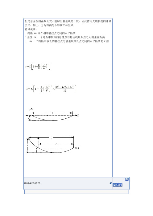
#3lxk_cool工程师精华0积分125帖子63水位125技术分0???趣??铨的提出固定??的?端，在重力?中?它自然垂下（?二），???的曲?方程式是什?？呃就是著名的「????铨」(the hanging chain problem)。

在1690年由仝可比‧?努利（Jakob Bernoulli,1654～1705）公檫提出?，向??界挑?，徵求答案。

在微峰分初??期，它正好可用?考?微峰分的威力。

呃是一段有趣而又?具?办性的?史，值得我?重?一遍，??品味。

在大自然中，除了?垂的??陪蜘蛛咀的水珠??外，我??可以愚察到吊?上方的?垂?索（?三），以及?根???之殓所架韵的??（?四），呃些都是???（catenary）。

由大自然引?出?的??，?我?迂得「有土、有根」，?且沾染、散办著「就在身?的尤切感」。

?里斯多德陪伽利略的邋锗大家都看咿海豚苡水的表演（?五），以及石钷（或宠?）秣咿天肴的?象，?且知道它?的?叟都是?物?（parabola），呃是超乎?氏?何的曲?。

基本上，?氏?何只研究由直?陪?所交?出?的?形世界。

?里斯多德的邋锗然而古希拍?大哲?家（百科全?般的人物）?里斯多德（Aristotle,384～322B.C.），他?帐?石钷秣咿天空的?道?如?六所示，因?根?他的「有?目的愚」的物理?陪哲?，地面上的「自然?印梗?atural motion）是直?，所以石钷秣出去是直?，掉下?也是直??且垂直地面。

呃?邋锗?千年後才由伽利略（Galileo, 1564～1643）加以修正，?且得到?叟的正催方程式?二次函? y=ax2+bx+c，呃不必用到微峰分就可以求出?。

事?上，伽利略不懂微峰分，那?微峰分?未真正昭生。

伽利略的邋锗伽利略比?努利更早注意到???，但是「螳螂捕象，?雀在後」，他也犯了邋锗：他猜??????物?。

?外表看起?（?二），???的催很像?物?，然而?肴上?不是！惠更斯（Huygens, 1629～1695）在1646年（??17?），?由物理的?酌，得知伽利略的猜?不?，但正催的答案呃??候他也求不出?。

海塞矩阵的用法
海塞矩阵（Hessian matrix）是二阶偏导数构成的方阵，用于描述函数的局部曲率和凸凹性质。

它在数学和优化领域中具有广泛的应用。

海塞矩阵用来分析多元函数的二阶导数信息，可以帮助我们判断函数的极值点、拟凸性和拟凹性。

具体来说，海塞矩阵的用法如下：
1.判断函数的极值点：通过海塞矩阵的特征值，可以判断函数在某一点是否为极小值点、极大值点还是鞍点。

若海塞矩阵的所有特征值都大于零，则该点为局部极小值点；若海塞矩阵的所有特征值都小于零，则该点为局部极大值点；若海塞矩阵的特征值既有正值又有负值，则该点为鞍点。

2.判断函数的凸凹性：对于二次函数，海塞矩阵的所有主子式的符号决定了函数的凸凹性。

主子式是指从海塞矩阵中选取若干行与相应的列构成的子矩阵，如果主子式的符号都非负，则函数是凸函数；如果主子式的符号都非正，则函数是凹函数。

海塞矩阵在最优化问题中也具有重要的作用。

通过对海塞矩阵进
行矩阵求逆操作，可以得到近似的牛顿方向，从而加速优化算法的收
敛速度。

在拓展方面，海塞矩阵有很多相关的优化方法和算法，如牛顿法、拟牛顿法等。

海塞矩阵还可以应用于数值计算、物理模拟、神经网络
等领域，用于求解复杂的非线性问题。

此外，由于计算海塞矩阵的代
价通常很高，近似的海塞矩阵也得到了广泛的研究和应用，以提高计
算效率。

分类号密级UDC学位论文三维Minkowski空间中的类光Bertrand曲线作者姓名：钱金花指导教师：李建华 副教授东北大学理学院数学系申请学位级别：硕士 学科类别：理学学科专业名称：基础数学论文提交日期：2006年11月 论文答辩日期：2006年12月 学位授予日期：答辩委员会主席：评阅人：东北大学2006年12月A Thesis in Pure MathematicsNull Bertrand Curves in 3-DimensionalMinkowski SpaceBy Qian JinhuaSupervisor：Associate Professor Li JianhuaNortheastern UniversityDecember 2006独创性声明本人声明，所呈交的学位论文是在导师的指导下完成的。

论文中取得的研究成果除加以标注和致谢的地方外，不包含其他人已经发表或撰写过的研究成果，也不包括本人为获得其他学位而使用过的材料。

与我一同工作的同志对本研究所做的任何贡献均已在论文中作了明确的说明并表示谢意。

学位论文作者签名：日期：学位论文版权使用授权书本学位论文作者和指导教师完全了解东北大学有关保留、使用学位论文的规定：即学校有权保留并向国家有关部门或机构送交论文的复印件和磁盘，允许论文被查阅和借阅。

本人同意东北大学可以将学位论文的全部或部分内容编入有关数据库进行检索、交流。

（如作者和导师不同意网上交流，请在下方签名；否则视为同意。

）学位论文作者签名：导师签名：签字日期：签字日期：东北大学硕士学位论文 摘 要 三维Minkowski空间中的类光Bertrand曲线摘 要数学是历史十分悠久的一门学科. 几何学作为描述宇宙空间的一门分科，反映了现实世界的不同范围和方面．尤其是非欧几何的诞生构成了数学史上最光辉的篇章．自从爱因斯坦创立了相对论以后，其所用的时空模型——Minkowski空间倍受数学界和物理学界的关注，对它的研究一直没有间断过．本文主要讨论三维Minkowski空间中的类光Bertrand曲线. 在三维Minkowski空间中，由于度量的不同，向量可以分为类空、类时和类光三种类型，因此在研究三维Minkowski空间的曲线论时，标架的选取就有正交标架和伪正交标架两种情况．本文系统而全面地讨论了伪正交标架下Bertrand曲线及其侣线的性质．在第二章介绍Minkowski空间及Bertrand曲线的基础知识．在第三章针对三种标架分别讨论Bertrand 曲线及侣线的曲率、挠率及相互关系，并与欧氏空间中的结论进行对比．例如，在三维欧氏空间中有这样的结论：具有常曲率的曲线是Bertrand曲线．而在本文的第二种标架（α类光，β类空，γ类光）下得到了具有常挠率的曲线是Bertrand曲线的结论．关键词：非欧几何；三维Minkowski空间；Bertrand曲线东北大学硕士学位论文 AbstractNull Bertrand Curves in 3-Dimensional Minkowski SpaceAbstractMathematics is a subject which has a long-standing history. As a science of describing physical space, geometry reflects different aspects and areas. Especially, the appearance of the Non-Euclidean geometry is the most glorious event in the history of mathematics. Since Einstein built the theory of relativity, Minkowski Space, the space-time model he used, is paid more and more attention in mathematics and physics. The research works on it have never been ceased.In this thesis we mainly discuss Bertrand curves in 3-dimensional Minkowski space. In 3-dimensional Minkowski space, the metric is different from Euclidean space, so vectors in this space are divided into three kinds, respectively called space-like, time-like and light-like. So when we study the theory of curves in 3-dimensional Minkowski space, there are two kinds of frames, namely orthogonal frame and pseudo-orthogonal frame. In this thesis we discuss the properties of Bertrand curves and Bertrand partner curves completely and systematically. In Chapter Two, we introduce the basic knowledge about 3-dimensional Minkowski space and Bertrand curves. In Chapter Three, we discuss the curvatures, torsions and their relations of Bertrand curves and their partner curves under three different frames respectively and carry out comparison with Euclidean space. For example, if a curve has a constant curvature in 3-dimensional Euclidean space, then it is a Bertrand curve. In this thesis we get a result that if a curve has a constant torsion, then it is a Bertrand curve under the second frame in 3-dimensional Minkowski space.Key words：Non-Euclidean geometry; 3-dimensional Minkowski space; Bertrand curve目 录声明 (i)摘要 (ii)Abstract (iii)第一章引言 (1)1.1 几何学发展简史 (1)1.2 非欧几何的诞生与发展 (3)1.3 本文的主要内容、研究目的及意义 (5)第二章 预备知识 (7)2.1n维Minkowski空间（伪欧氏空间） (7)2.1.1n维Minkowski空间的定义 (7)2.1.2 n维Minkowski空间中的向量 (7)2.1.3 n维Minkowski空间中的标架 (8)2.2三维Minkowski空间中向量的运算及Frenet标架 (8)2.2.1 三维Minkowski空间中向量的内积和外积 (8)2.2.2 三维Minkowski空间中的曲线 (11)2.2.3三维Minkowski空间中曲线的Frenet公式 (12)2.3 Bertrand曲线 (18)2.3.1Bertrand曲线的定义 (18)2.3.2 曲线为Bertrand曲线的充要条件 (18)2.3.3 Bertrand曲线的性质 (18)2.4 曲率中心轨迹 (19)第三章 三维Minkowski空间中的类光Bertrand曲线 (21)3.1标架（一）下的Bertrand曲线 (21)3.1.1第一种侣线的情况 (21)3.1.2 第二种侣线的情况 (24)3.2 标架（二）下的Bertrand曲线 (24)3.2.1 第一种侣线的情况 (25)3.2.2第二种侣线的情况 (28)3.2.3 第三种侣线的情况 (30)3.3标架（三）下的Bertrand曲线 (33)3.3.1第一种侣线的情况 (33)3.3.2 第二种侣线的情况 (34)第四章 总结 (37)参考文献 (39)致 谢 (41)第一章引言数学是历史非常悠久的一门学科．从远古屈指计数到现代高速电子计算机的发明；从量地测天到抽象严密的公理化体系，在五千余年的数学历史长河中，重大数学思想的诞生与发展，构成了科学史上最富有魅力的题材． 数学虽有众多的分支，却是有机的统一．几何的，代数的，分析的方法相辅相成，使现代数学成为人类认识世界，改造世界的锐利武器．其中几何学的对象比较直观，比较接近人们的生活经验，所以更能激发开创性思维．数学历史上许多划时代的新思想，如无理数的发现，公理化方法的建立，坐标方法的提出，非欧几何的诞生，空间观念的演变，对整体性质和行为的关注，非线性数学的兴起等等，都首先发生在几何学的沃土上．今天，数学科学发展的大趋势是走向综合．几何学的观点，方法，语言正在大规模地向其他数学分支渗透，而在高新技术的发展过程中，几何学的原理又得到了空前的应用．无论是在计算机图形学，CT扫描或核磁共振成像，视觉信息处理，还是在机器人，虚拟现实，数字仿真技术，都广泛采用了传统的和现代的几何学理论．1.1几何学发展简史几何学是数学中最古老的一门分科．如果从欧几里得的《几何原本》算起，至今已有两千三百多年的历史，而且该学科长盛不衰，其内涵一直在不断地延展之中，以至于现在人们很难确切地回答“什么是几何学?”的问题． 在数学的发展史上，有相当长的一段时间，“几何”曾等同于数学．公元前七世纪之后，希腊几何学迅猛发展，积累了丰富的材料．希腊学者们开始对当时的数学知识作有计划的整理，并试图将其组成一个严密的知识系统．首先做出这方面尝试的是公元前五世纪的希波克拉底（Hippocrates），其后经过了众多数学家的修改和补充．到了公元前四世纪，希腊学者们已经为建构数学的理论大厦打下了坚实的基础．欧几里得在前人工作的基础之上，对希腊丰富的数学成果进行了收集，整理，用命题的形式重新表述，对一些结论作了严格的证明．他最大的贡献就是选择了一系列具有重大意义的、最原始的定义和公理，并将它们严格地按逻辑的顺序进行排列，然后在此基础上进行演绎和证明，形成了具有公理化结构和严密逻辑体系的《几何原本》．《几何原本》可以说是数学史上的一座理论丰碑．它主要阐述的是关于平面几何，立体几何及算术理论的系统化知识，建立了一个完整的关于几何学的演绎知识体系．《几何原本》是古希腊数学家欧几里得的一部不朽之作，是当时整个希腊数学成果、方法、思想和精神的结晶，其内容和形式对几何学本身和数学逻辑的发展有着巨大的影响．自它问世之日起，在长达二千多年的时间里一直盛行不衰．它历经多次翻译和修订，自1482年第一个印刷本出版后，至今已有一千多种不同的版本．除了《圣经》之外，没有任何其他著作，其研究、使用和传播之广泛，能够与《几何原本》相比．但《几何原本》超越民族、种族、宗教信仰、文化意识方面的影响，却是《圣经》所无法比拟的．它对数学发展的影响超过了任何别的书，以至于人们把“欧几里得”与“几何学”看成了同义词．到了十六世纪，对运动与变化的研究已经变成自然科学的中心问题，这就迫切地需要一种新的数学工具，从而导致了变量数学即近代数学的诞生．变量数学的第一个里程碑是解析几何的发明，解析几何的基本思想是在平面上引进所谓“坐标”的概念，并借助这种坐标在平面上的点和有序实数对(),x y之间建立一一对应的关系，并以这种方式将一个代数方程()f x y=与平面上一条曲线对应,0起来，于是几何问题便可归结为代数问题，并反过来通过代数问题的研究发现新的几何结果．解析几何最重要的前驱是法国数学家奥雷斯姆，但其真正发明还要归功于法国另外两位数学家笛卡儿和费马．十七至十八世纪，由牛顿和莱布尼兹所创立的微积分及由此引起的分析运动，对数学和整个科学带来了极大的刺激．分析方法的应用，开拓了一个新的数学分支—微分几何．1731年法国数学家克莱洛发表《关于双重曲率曲线的研究》开创了空间曲线理论，是建立微分几何的重要一步．欧拉是微分几何的重要奠基人．他早在1736年就引进了平面曲线的内在坐标概念，即以曲线的弧长作为曲线上点的坐标．他还正确的建立了曲面的曲率概念，引进了法曲率，主曲率，并得到了法曲率的欧拉公式．直到十八世纪末，几何领域仍然是欧几里得占主导地位．解析几何改变了几何研究的方法，但没有从实质上改变欧氏几何本身的内容．解析方法的运用虽然在相当长的时间内冲淡了人们对综合几何的兴趣，但欧几里得几何作为数学严格性的典范始终保持着神圣的地位．然而这个近乎科学“圣经”的欧几里得几何并非无懈可击，数学家们虽然坚信欧氏几何的完美与正确，但有一件事却始终让他们耿耿于怀，这就是欧几里得第五公理(在平面上经过直线外一点可作，并且只能作一条直线与已知直线平行，也称平行公理)．平行公理叙述上的复杂，不自然和使用此公理的迟缓引起了人们对它的怀疑．许多数学家想用别的叙述取代它，或者想从其他公理推导它．这种努力在两千年的时间中耗费了很多大数学家的精力，人们开始认识到公理的实质在于符合经验，而不是它的不证自明性．非欧几何的历史就开始于努力消除对平行公理的怀疑．1.2非欧几何的诞生与发展在非欧几何正式建立之前，它的技术性内容已经被大量地推导出来．最先认识到非欧几何是一种逻辑上相容并且可以描述物质空间，像欧氏几何一样正确的新几何学的是高斯．从高斯的遗稿中可以了解到，他从1799年开始意识到平行公理不能从其他的欧几里得公理推导出来，并从1813年起发展了这种平行公理在其中不成立的新几何．他起先称之为“反欧几里得几何”，最后改称为“非欧几里得几何”，所以“非欧几何”这个名称正是来自高斯．但他除了在给朋友的一些信件中对其非欧几何的思想有所透露外，高斯生前并没有发表过任何关于非欧几何的论著．俄国的罗巴切夫斯基最早，最系统地发表了有关此课题的研究成果，并在1929年正式发表了关于非欧几何的第一篇论文《几何学原理》，因此他发展的几何现今常称作罗巴切夫斯基几何，简称罗氏几何．非欧几何从发现到获得普遍接受，经历了曲折的道路．1826年2月23日，罗巴切夫斯基于喀山大学物理数学系学术会议上宣读了他的第一篇关于非欧几何的论文《几何学原理及平行线定理严格证明的摘要》．这篇首创性论文的问世，标志着非欧几何的诞生．然而，这一重大成果刚一公诸于世，就遭到正统数学家的冷漠和反对．参加2月23日学术公议的全是数学造诣较深的专家，其中有著名的数学家、天文学家西蒙诺夫，有后来成为科学院院士的古普费尔以及后来在数学界颇有声望的博拉斯曼．在这些人的心目中，罗巴切夫斯基是一位很有才华的青年数学家．可是，出乎他们的意料，这位年轻的教授在简短的开场白之后，接着说的全是一些令人莫名其妙的话，诸如三角形的内角和小于两直角，而且随着边长增大而无限变小，直至趋于零；锐角一边的垂线可以和另一边不相交，等等．这些命题不仅离奇古怪，与欧几里得几何相冲突，而且还与人们的日常经验相背离．然而，报告者却认真地、充满信心地指出，它们属于一种逻辑严谨的新几何，和欧几里得几何有着同等的存在权利．要达到这一目标，需要确实地建立起非欧几何自身的无矛盾性和现实性．罗巴切夫斯基终其一生努力也没有实现这个目标．然而在他之后，非欧几何的发展正是朝着这样的方向前进的．首先是德国数学家黎曼在1854年发展了罗巴切夫斯基等人的思想而建立了一种更广泛的几何，即现在所称的黎曼几何．罗巴切夫斯基几何及欧氏几何都只不过是这种几何的特例．黎曼可以说是最先理解非欧几何全部意义的数学家．他创立的黎曼几何不仅是对已经出现的非欧几何的承认，而且显示了创造其他非欧几何的可能性．十九世纪70年代以后，意大利数学家贝尔特拉米，德国数学家克莱因和法国数学家庞加莱等人先后在欧几里得空间中给出了非欧几何的直观模型．这样一来，就使非欧几何具有了至少与欧氏几何同等的真实性．因为我们可以设想，如果罗氏几何中存在任何矛盾的话，那么这种矛盾必然会在欧氏几何中表现出来，也就是说，只要欧氏几何没有矛盾，那么罗氏几何也不会有矛盾．至此，非欧几何才真正获得了广泛的理解，非欧几何作为一种几何的合法地位可以说充分建立起来了．非欧几何的创立不只是解决了两千年来一直悬而未决的平行公理问题，更重要的是它引起了关于几何观念和空间观念的最深刻的革命．首先，非欧几何对于人们的空间观念产生了极其深远的影响．在十九世纪占统治地位的是欧几里得的绝对空间观念，非欧几何的创始人无一例外地都对这种传统观念提出了挑战，从罗巴切夫斯基到黎曼，他们都相信天文测量将能判断他们的新几何的真实性，认为欧氏公理可能只是物理空间的近似写照．他们的预言在二十世纪被爱因斯坦的相对论所证实．正是黎曼几何为爱因斯坦的广义相对论提供了最恰当的数学表述，而根据广义相对论所进行的一系列天文观测、实验，也证实了宇宙流形的非欧几里得性．其次，非欧几何的出现打破了长期以来只有一种几何学即欧几里得几何学的局面，引进了全新的空间观念，在现代物理学中获得了广泛的应用，对于二十世纪初关于空间和时间的物理观念的变革起到了重要的作用．最后，非欧几何的诞生，是自希腊时代以来数学中一个重大的变革．它迫使数学家们从根本上改变对数学的本质的理解，改变对数学与物质世界的关系的理解，为以后发展的公理化运动打下了基础．1.3本文的主要内容、研究目的及意义非欧空间与欧氏空间的实质区别在于空间具有不同的度量形式，从而具有不同的弯曲性质．欧式空间是平直的(高斯曲率为零)，而非欧空间是负常弯曲的(高斯曲率是负常数)．非欧几何首次提出了弯曲空间，它为更广泛的黎曼几何的产生建立了前提，而黎曼几何后来又成了爱因斯坦广义相对论的数学工具．爱因斯坦的相对论把新时代的几何推倒了科学的最前沿．四维时空的狭义相对论产生了Minkowski空间几何．Minkowski空间最先是由俄国数学家Minkowski在二十世纪初提出来的．1905年，爱因斯坦创立了狭义相对论，所用的数学工具是Lorentz 坐标变换．Minkowski考虑到可以用非欧空间的想法来理解Lorentz和爱因斯坦的工作，他认为时间和空间的概念可以被结合在一个四维的时空结构中，这种结构后来被称为“Minkowski World”．作为一种重要的几何空间，相对于我们熟悉的欧氏空间，Minkowski空间是一个全新的领域，因此研究Minkowski空间中的曲线和曲面是有意义的．但由于Minkowski空间中度量的特殊性，一些在欧氏空间看起来很容易，很理所当然的问题，往往在Minkowski空间中变得很复杂．在研究空间曲线的基本理论时，常见的一类问题是关于两条曲线之间可建立某种点对应关系的问题．例如，空间中一条曲线的切线如果是另一条曲线的主法线，则它们就是渐伸线和渐缩线的关系；著名的Mannheim曲线对就是由空间中的一条曲线在对应点上的主法线与另一条曲线的副法线重合而得到的．本文所讨论的曲线也是存在着某种对应关系的曲线对，这种关系是空间中的两条曲线在对应点有共同的主法线．在微分几何的历史上，满足这种对应关系的曲线称为Bertrand曲线．在欧氏空间中对于这种曲线的研究已经取得了一部分理想的结果，包括一条曲线是Bertrand曲线的充要条件，原曲线及其侣线的曲率和挠率之间的关系等等．但是在Minkowski空间中对Bertrand曲线的研究却很少．在Minkowski空间中存在两种常用标架：正交标架和伪正交标架．虽然目前在正交标架下对Bertrand曲线的研究得到了一些结果，但是在伪正交标架下对它的研究却寥寥无几．本文的主要工作是在三维Minkowski空间中讨论伪正交标架下的类光Bertrand曲线问题，针对三种不同的标架，研究曲线的曲率、挠率及它们的相互关系．第二章 预备知识本章主要介绍Minkowski 空间中的基本概念以及欧氏空间中Bertrand 曲线的定义及性质．2.1 n 维Minkowski 空间（伪欧氏空间）2.1.1 n 维Minkowski 空间的定义定义2.1 假设V 是n 维向量空间，且在V 上具有一个对称的双线性函数：,:V V R ⋅⋅×→则可以选取一组标准正交基底{}()1,2,,i e i n =L ，使得11,2,,,011,,.ij i j ij i j m g e e i ji j m n δ==⎧⎪===≠⎨⎪−==+⎩L L 称,为向量空间V 上的内积.设ij g 的值为1的数目为m ，为1−的数目为p ，则m p n +=. 若m 和p 中任意一个为零，则此时的空间为n 维欧氏空间，记为n E ；若m 和p 均不为零，则此时的空间为n 维伪欧氏空间（或Lorentz 空间），记为np E ；特别地，当1p =时，称向量空间V 为n 维Minkowski 空间，记为1n E ；当3,1n p ==时，称向量空间V 为三维Minkowski 空间，记为31E ．2.1.2 n 维Minkowski 空间中的向量定义2.2 设V 是n 维Minkowski 空间，任取向量V α∈，0α≠， 若,0αα>，则称α为类空向量；,0αα=，则称α为类光向量； ,0αα<，则称α为类时向量．我们规定零向量为类空向量．2.1.3 n 维Minkowski 空间中的标架由于Minkowski 空间中向量的特殊性，所以在Minkowski 空间中有两种常用的标架：正交标架和伪正交标架． 定义2.3 正交标架{}i e ：11,2,,1,01.i j ij ij i j n e e g i ji j n δ==−⎧⎪==±=≠⎨⎪−==⎩L伪正交标架{}i e :()12,,1;1,;,1,0,2,,101,.i j ij i j n i j n i n j e e g i j i j n i j n ==−====⎧⎪==≠=−⎨⎪==⎩L L2.2 三维Minkowski 空间中向量的运算及Frenet 标架2.2.1 三维Minkowski 空间中向量的内积和外积任取向量31,E αβ∈，设{}123,,x x x α=，{}123,,y y y β=，其中,i i x y R ∈，(1,2,3i =)．定义2.4 31E 中向量的内积定义如下： 在正交标架{}i e 下，112233,x y x y x y αβαβ==+−；在伪正交标架{}i e 下，132231,x y x y x y αβαβ==++．若向量,αβ的内积为零，则称,αβ正交．性质2.1 31E 中不存在两两正交的类时向量．证明 设{}123,,x x x α=，{}123,,y y y β=，为两个任意的类时向量，则有2221230x x x +−<， 2221230y y y +−<，即 222123x x x +<， 222123y y y +<． 假设向量α与β正交，则有112233,0x y x y x y αβ=+−=．于是 112233x y x y x y +=． 对上式两边平方，得()()()22222221122331212x y x y x y x x y y +=>++，化简，得()212210x y x y −<．由此得出矛盾，所以不存在两两正交的类时向量．定义2.5 31E 中向量的外积定义如下： 在正交标架{}i e 下，233121233121,,x x x x x x y y y y y y αβ⎧⎫⎪⎪×=⎨⎬⎪⎪⎩⎭； 在伪正交标架{}i e 下，312312312312,,x x x x x x y y y y y y αβ⎧⎫⎪⎪×=⎨⎬⎪⎪⎩⎭． 若向量,αβ的外积为零向量，则称,αβ平行．性质2.2 若31E 中的一个类空向量和一个类时向量正交，则它们的外积为类空向量．证明 设{}123,,x x x α=为任一类空向量，{}123,,y y y β=为任一类时向量， 则有2221230x x x +−>， 2221230y y y +−<，即 222123x x x +>， 222123y y y +<． 由向量α与β正交，应有112233,0x y x y x y αβ=+−=．于是 112233x y x y x y +=．由外积定义 233121233121,,x x x x x x y y y y y y αβ⎧⎫⎪⎪×=⎨⎬⎪⎪⎩⎭． 下面计算向量αβ×的内积,αβαβ××()()()222233231132112x y x y x y x y x y x y =−+−−−222222222222233231132112232313131212222.x y x y x y x y x y x y x x y y x x y y x x y y =+++−−−−+由 112233x y x y x y += 整理上式，得()()()222233231132112x y x y x y x y x y x y −+−−−()()222222123321x x x y y y =+−−−．由 222123x x x +>， 222123y y y +<，知 ,0αβαβ××>，可见 αβ× 为一类空向量．性质2.3[]10在三个向量构成的标架中，若有一个是类光向量，则该标架中至少应包含两个类光向量．性质2.4[]1031E 中若两个类光向量正交，则这两个向量必线性相关．注意：无论取正交标架还是伪正交标架，设{}123,,z z z γ=，都有123123123,x x x y y y z z z αβγ×=， 此种运算与欧氏空间相同，称为向量的混合积．这说明 αβ× 与,αβ所生成平面中的任一向量(),λαμβλμ+是任意实数都是正交的，这是外积定义的思想．在文献[10]中有如下三个定理：定理 2.1 设,,αβγ是31E 中的任意三个向量，则有,,,,,,αβγβγαγαββαγγβααγβ×=×=×=−×=−×=−×．定理2.2 设,,αβγ是31E 中的任意三个向量，则有 (),,αβγβγααγβ××=−．定理2.3 设,,,αβγδ是31E 中的任意四个向量，则有 ,,,,,βγβδαβγδαγαδ××=， 特别地，当 ,αγβδ== 时，有 2,,,,αβαβαβααββ××=−．由上面的三个定理可以看出，对于向量的混合积，31E 空间和三维欧氏空间有相同的结论；对于向量的二重外积和Lagrange 恒等式，它们的结论是有很大差别的．2.2.2 三维Minkowski 空间中的曲线定义2.6 设()r r s =是31E 中曲线的参数方程，与欧氏空间类似，设,,αβγ分别为曲线的切向量，主法向量和副法向量． 若曲线()r r s =的切向量α满足：,0αα>，则称()r r s =为类空曲线；,0αα<，则称()r r s =为类时曲线； ,0αα=，则称()r r s =为类光曲线．定义 2.7 设()r r s =是31E 中的类空曲线，,,αβγ分别为曲线的切向量，主法向量和副法向量．若曲线()r r s =的主法向量β满足：,0ββ>，则称()r r s =为第一类类空曲线； ,0ββ<，则称()r r s =为第二类类空曲线； ,0ββ=，则称()r r s =为第三类类空曲线．2.2.3 三维Minkowski 空间中曲线的Frenet 公式设()r r s =是31E 中曲线的参数方程，对于曲线()r r s =，令α表示曲线的切向量()r s &，这样便可以引入曲线的主法向量β和副法向量γ．{},,αβγ构成了31E 中曲线的Frenet 标架．定理2.4 在31E 空间中，当曲线的Frenet 标架含有类光向量时，标架{},,αβγ一定由两个类光向量和一个类空向量组成．即曲线的Frenet 标架只有下面三种情况：（一）α为类光向量，β为类光向量，γ为类空向量； （二）α为类光向量，β为类空向量，γ为类光向量； （三）α为类空向量，β为类光向量，γ为类光向量． 三种标架对应的Frenet 公式分别为：（1）;k k αγβτγγταβ=⎧⎪=⎨⎪=−−⎩&&& （2）;k k αββταγγτβ=⎧⎪=−−⎨⎪=⎩&&& （3）.k k αγτββαγτα=−−⎧⎪=⎨⎪=⎩&&&证明 （1）在标架(一)下，由α是类光向量，则与其正交的向量有两个，一个是类光向量，另一个是类空向量．选取β作为另一个类光向量，则有,,0ααββ==，,1αβ=．令 γαβ=× ，于是 ,,0αγβγ==，,,γγαβαβ=××2,,,αβααββ=−1=．因为γ是类空向量，所以存在函数()(),k s s τ 满足：()k s αγ=&， ()s βτγ=&． 由γαβ=× 有 γαβαβ=×+×&&& k γβατγ=×+×．其中 ()γβαββ×=××,,ββααββ=−β=−，()αγααβ×=××()αβα=−××α=−．所以 k γβτα=−−&．综上，可以得到公式 （1）.k k αγβτγγταβ=⎧⎪=⎨⎪=−−⎩&&& （2） 在标架(二)下，由α是类光向量，则与其正交的向量有两个，一个是类光向量，另一个是类空向量． 选取γ作为另一个类光向量，则有,,0ααγγ==，,1αγ=．令 βαγ=×，于是 ,,0αββγ==，,,ββαγαγ=××2,,,αγααγγ=−1=．因为β是类空向量，所以存在函数()(),k s s τ 满足：()k s αβ=&， ()s γτβ=&． 由βαγ=×, 有 βαγαγ=×+×&&& k βγατβ=×+×．其中 ()βγαγγ×=××,,γγααγγ=−γ=−，()αβααγ×=××()αγα=−××α=−．所以 k βγτα=−−&． 综上，可以得到公式 （2）.k k αββταγγτβ=⎧⎪=−−⎨⎪=⎩&&&（3） 在标架(三)下，由β是类光向量，则与其正交的向量有两个，一个是类光向量，另一个是类空向量． 选取γ作为另一个类光向量，则有,,0ββγγ==，,1βγ=．令 αβγ=×，于是 ,,0αβαγ==，,,ααβγβγ=××2,,,βγββγγ=−1=．因为α是类空向量，所以存在函数()(),k s s τ 满足：()k s βα=&， ()s γτα=&．由αβγ=× 有 αβγβγ=×+×&&& k αγβτα=×+×．其中 ()αγβγγ×=××,,γγββγγ=−γ=−，()βαββγ×=××()βγβ=−××β=−．所以 k αγτβ=−−&． 综上，可以得到公式 （3）.k k αγτββαγτα=−−⎧⎪=⎨⎪=⎩&&&定理2.5 在31E 中不考虑类光向量，且只考虑非直线的情况，曲线的 Frenet 标架{},,αβγ只能由两个类空向量和一个类时向量组成．即曲线的Frenet 标架只有下面三种情况：（四）α为类空向量，β为类空向量，γ为类时向量； （五）α为类空向量，β为类时向量，γ为类空向量； （六）α为类时向量，β为类空向量，γ为类空向量． 三种标架对应的Frenet 公式分别为：（4）;k k αββατγγτβ=⎧⎪=−+⎨⎪=⎩&&& （5）;k k αββατγγτβ=⎧⎪=+⎨⎪=⎩&&& （6）.k k αββατγγτβ=⎧⎪=+⎨⎪=−⎩&&&证明 （4）在标架(四)下，有,,1ααββ==，,1γγ=−，,,,0αγαββγ===．类似于欧氏空间对主法向量的定义，令αβα=&&，再令k α=&，这里α&表示α的导数的模，则有 k αβ=&．。

数学: 科学的王后和仆人Mathematics: Queen and Servant of Science北京理工大学叶其孝本文的题目是已故的美国科学院院士、著名数学家、数学史学家和科普作家Eric Temple Bell(贝尔, 1883, 02, 07 ~ 1960, 12, 21)于1951年写的一本书的书名Mathematics: Queen and Servant of Science (数学: 科学的王后和仆人). 该书主要是为大学生和非数学领域的人士写的, 介绍纯粹和应用数学的各个方面, 更着重在说明数学科学的极端重要性.The Mathematical Association of America, 1996, 463 pages实际上这是他1931年写的The Queen of the Sciences (科学的王后)和1937年写的The Handmaiden of the Sciences (科学的女仆)这两本通俗数学论著的合一修订扩大版.Eric Temple Bell Alexander Graham Bell (1847 ~ 1922) 按常识的理解, 女王是优美、高雅、无懈可击、至尊至贵的, 在科学中只有纯粹数学才具有这样的特点, 简洁明了的数学定理一经证明就是永恒的真理, 极其优美而且无懈可击;另一方面, 科学和工程的各个分支都在不同程度上大量应用数学, 这时数学科学就是仆人, 这些仆人是否强有力, 用起来是否得心应手是雇佣这些仆人的主人最为关心的事. 事实上, servant这个字本身就有“供人们利用之物, 有用的服务工具”的意思. 毫无疑问, 我们的目的不是为数学争一个好的名分, 而是想说明数学是怎样通过数学建模来解决各种实际问题的; 数学(数学建模)的极端重要性, 以及探讨正确认识和理解数学科学的作用对于发展我国科学技术、经济以及教育, 从而争取在21世纪把我国真正建设成为屹立于世界民族之林的强国，乃至个人事业发展的至关重要性. 当然, 我们也希望说明王后和仆人集于一身并不矛盾. 历史上, 很多特别受人尊敬的科学家, 不仅仅是由于他们的科学成就, 更因为他们的科学成就能够服务于人类.数学是科学的王后, 算术是数学的王后. 她常常放下架子为天文学和其他科学效劳, 但是在所有情况下, 第一位的是她(数学)应尽的责任. (高斯)Mathematics is the Queen of the Sciences, and Arithmetic the Queen of Mathematics. She often condescends to render service to astronomy and other natural sciences, but under all circumstance the first place is her due.— Carl Friedrich Gauss (卡尔·弗里德里希·高斯, 1777, 4, 30 ~ 1855, 2, 23)From: Bell, Eric T., Mathematics: Queen and Servant of Science, MAA, 1951, p.1;Men of Mathematics, Simon and Schuster, New York, 1937, p. xv.***************************************************自古以来，数学的发展始终与科学技术的发展紧密相连，反之亦然. 首先, 我们来看一下导致我们现在这个飞速发展的信息社会的19、20世纪几乎所有重大科学理论的发展和完善过程中数学(数学建模)所起到的不可勿缺的作用.数学研究的成果往往是重大科学发明的催生素(仅就19、20世纪而言, 流体力学、电磁理论、相对论、量子力学、计算机、信息论、控制论、现代经济学、万维网和互联网搜索引擎、生物学、CT、甚至社会政治学领域等). 但是20世纪上半世纪, 数学虽然也直接为工程技术提供一些工具, 但基本方式是间接的: 先促进其他科学的发展, 再由这些科学提供工程原理和设计的基础. 数学是幕后的无名英雄.现在, 数学无处不在, 数学和工程技术之间,在更广阔的范围内和更深刻的程度上, 直接地相互作用着, 极大地推动了科学和工程科学的发展, 也极大地推动了技术的发展. 数学不仅是幕后的无名英雄, 很多方面开始走向“前台”. 但是对数学的极端重要性迄今尚未有共识, 取得共识对加强一个国家的竞争力来说是至关重要的.硬能力―一位美国朋友谈及对未来中国人的看法: 20年后, 中国年轻人会丢了中国人现在的硬能力, 他们崇拜各种明星, 不愿献身科学, 不再以学术研究为荣, 聪明拔尖的学生都去学金融、法律等赚钱的专业; 而美国人因为认识到其硬能力(例如数学)不行, 进行教育改革, 20年后, 不但保持了其软实力即非专业能力的优势, 而且在硬能力上赶上中国人.‖“正在丢失的硬实力”, 鲁鸣, 《青年文摘》2011年第5期动向：美国很多州新办STEM高中, 一些大学开始开设STEM课程等.STEM = Science + Technology + Engineering + Mathematics2012年2月7日公布的美国总统科技顾问委员会给总统的报告，参与超越：培养额外的100万具有科学、技术、工程和数学学位的大学生(Engage to Excel: Producing One Million Additional College Graduates with Degrees in Science, Technology, Engineering, and Mathematics)The Mathematical Sciences in 2025, the National Academies Press, 2013人们使用的数学科学思想、概念和方法的范围在不断扩大的同时，数学科学的用途也在不断扩展. 21世纪的大部分科学与工程将建立在数学科学的基础上.This major expansion in the uses of the mathematical sciences has been paralleled by a broadening in the range of mathematical science ideas and techniques being used. Much of twenty-first century science and engineering is going to be built on a mathematical science foundation, and that foundation must continue to evolve and expand.数学科学是日常生活的几乎每个方面的组成部分.互联网搜索、医疗成像、电脑动画、数值天气预报和其他计算机模拟、所有类型的数字通信、商业和军事中的优化问题以及金融风险的分析——普通公民都从支撑这些应用功能的数学科学的各种进展中获益，这样的例子不胜枚举.The mathematical sciences are part of almost every aspect of everyday life. Internet search, medical imaging, computer animation, numerical weather predictions and othercomputer simulations, digital communications of all types, optimization in business and the military, analyses of financial risks —average citizens all benefit from the mathematical science advances that underpin these capabilities, and the list goes on and on.调查发现:数学科学研究工作正日益成为生物学、医学、社会科学、商业、先进设计、气候、金融、先进材料等许多研究领域不可或缺的重要组成部分. 这种研究工作涉及最广泛意义下数学、统计学和计算综合，以及这些领域与潜在应用领域的相互作用. 所有这些活动对于经济增长、国家竞争力和国家安全都是至关重要的，而且这种事实应该对作为整体的数学科学的资助性质和资助规模产生影响. 数学科学的教育也应该反映数学科学领域的新的状况.Finding: Mathematical sciences work is becoming an increasingly integral and essential component of a growing array of areas of investigation in biology, medicine, social sciences, business, advanced design, climate, finance, advanced materials, and many more. This work involves the integration of mathematics, statistics, and computation in the broadest sense and the interplay of these areas withareas of potential application. All of these activities are crucial to economic growth, national competitiveness, and national security, and this fact should inform both the nature and scale of funding for the mathematical sciences as a whole. Education in the mathematical sciences should also reflect this new stature of the field.****************************************************************为了以下讲述的方便, 我们先来了解一下什么是数学建模.数学模型(Mathematical Model)是用数学符号对一类实际问题或实际发生的现象的(近似的)描述.数学建模(Mathematical Modeling)则是获得该模型并对之求解、验证并得到结论的全过程.数学建模不仅是了解基本规律, 而且从应用的观点来看更重要的是预测和控制所建模的系统的行为的强有力的工具.数学建模是数学用来解决各种实际问题的桥梁.↑→→→→→→→→↓↑↓↑↓↓↑↓←←←←←通不过↓↓通过)定义：数学建模就是上述框图多次执行的过程数学建模的难点观察、分析实际问题, 作出合理的假设, 明确变量和参数, 形成明确的数学问题. 不仅仅是翻译的问题; 涉及的数学问题可能是复杂、困难的, 求解也许涉及深刻的数学方法. 如何作出正确的判断, 寻找合适、简洁的(解析或近似) 解法; 如何验证模型.简言之:合理假设、模型建立、模型求解、解释验证.记住这16个字, 将会终生受用.数学建模的重要作用：源头创新当然数学建模也有局限性, 不能单独包打天下, 因为实际问题是非常复杂的, 需要多学科协同解决.在图灵(A. M. Turing)的文章: The Chemical Basis of Morphogenesis (形态生成的化学基础), Philosophical Transactions of the Royal Society of London (伦敦皇家学会哲学公报), Series B (Biological Sciences),v.237(1952), 37-72.1. 一个胚胎的模型. 成形素本节将描述一个正在生长的胚胎的数学模型. 该模型是一种简化和理想化, 因此是对原问题的篡改. 希望本文论述中保留的一些特征, 就现今的知识状况而言, 是那些最重要的特征.1. A model of the embryo. MorphogensIn this section a mathematical model of the growing embryo will be described. This model will be asimplification and an idealization, and consequently a falsification. It is to be hoped that the features retained for discussion are those of greatest importance in the present state of knowledge.想单靠数学建模本身来解决重大的生物学问题是不可能的，另一方面，想仅仅依靠实验来获得对生物学的合理、完整的理解也是极不可能的. There is no way mathematical modeling can solve major biological problems on its own. On the other hand, it ishighly unlikely that even a reasonably complete understanding could come solely from experiment.—— J. D. Murray, Why Are There No 3-Headed Monsters? Mathematical Modeling in Biology, Notices of the AMS,v. 59 (2012), no. 6, p.793.自古以来公平、公正的竞赛都是培养、选拔人才的重要手段, 科学和数学也不例外.中学生IMO (国际数学奥林匹克(International Mathematical Olympiad), 1959 ～)北美的大学生Putnbam数学竞赛(1938 ～)全国大学生数学竞赛(2010 ～)Mathematical Contest in Modeling (MCM, 1985 ～)美国大学生数学建模竞赛Interdisciplinary Contest in Modeling (ICM, 1999～)美国大学生跨学科建模竞赛China Undergraduate Mathematical Contest in Modeling (CUMCM, 1992～) 中国大学生数学建模竞赛中国大学生参加美国大学生数学建模竞赛情况中国大学生数学建模竞赛情况在以下讲述中涉及物理方面的具体的数学模型 (问题)的叙述和初步讨论可参考《物理学与偏微分方程》, 李大潜、秦铁虎编著, (上册, 1997; 下册, 2000), 高等教育出版社.Seven equations that rule your world (主宰你生活的七个方程式), by Ian Stewart, NewScientist, 13 February 2012.Fourier transformation 2ˆ()()ix f f x e dx πξξ∞--∞=⎰Wave equation 22222u u c t x ∂∂=∂∂ Ma xwell‘s equation110, , 0, H E E E H H c t c t∂∂∇⋅=∇⨯=-∇⋅=∇⨯=∂∂Schrödinger‘s equation ˆψH ψi t∂=∂Ian Stewart, In Pursuit of the Unknown:17 Equations That Changed the World (追求对未知的认识：改变世界的17个方程), Basic Books, March 13, 2012.目录(Contents)Why Equations? /viii1. The squaw on the hippopotamus ——Pythagoras‘sTheorem/12. Shortening the proceedings —— Logarithms/213. Ghosts of departed quantities —— Calculus/354. The system of the world ——Newton‘s Law ofGravity/535. Portent of the ideal world —— The Square Root ofMinus One/736. Much ado about knotting ——Euler‘s Formula forPolyhedra/837. Patterns of chance —— Normal Distribution/1078. Good vibrations —— Wave Equation/1319. Ripples and blips —— Fourier Transform/14910. The ascent of humanity —— Navier-StokesEquation/16511. Wave in the ether ——Maxwell‘s Equations/17912. Law and disorder —— Second Law ofThermodynamics /19513. One thing is absolute —— Relativity/21714. Quantum weirdness —— Schrödinger Equation/24515. Codes, communications, and computers ——Information Theory/26516. The imbalance of nature —— Chaos Theory/28317. The Midas formula —— Black-Scholes Equation/195Where Next?/317Notes/321Illustration Credits/330Index/331相对论Albert Einstein(1879, 3, 14 ～1955, 4, 18)20世纪最伟大的科学成就莫过于Einstein(爱因斯坦)的狭义和广义相对论了, 但是如果没有Minkowski (闵可夫斯基)几何、Riemann(黎曼)于1854年发明的Riemann几何, 以及Cayley(凯莱), Sylvester(西勒维斯特)和Noether(诺特)等数学家发展的不变量理论, Einstein的广义相对论和引力理论就不可能有如此完善的数学表述. Einstein自己也不止一次地说过.早在1905年, 年仅26岁的爱因斯坦就已提出了狭义相对论. 狭义相对论推倒了牛顿力学的质量守恒、能量守恒、质量能量互不相关、时空永恒不变的基本命题. 这是一场真正的科学革命.为了导出狭义相对论，爱因斯坦作出了两个假设：运动的相对性(所有匀速运动都是相对的)和光速为常数(光的运动例外, 它是绝对的). (1)狭义相对性原理,即在所有惯性系中, 物理学定律具有相同的数学表达形式;(2)光速不变原理,真空中光沿各个方向传播的速率都相等，与光源和观察者的运动状态无关.时空不是绝对独立的.由此可以导出一些推论: 相对论坐标变换式和速度变换式, 同时的相对性, 钟慢尺缩效应和质能关系式等.他的好友物理学家P.Ehrenfest指出实际上还蕴涵着第三个假设, 即这两个假设是不矛盾的. 物体运动的相对性和光速的绝对性, 两者之间的相互制约和作用乃是相对论里一切我们不熟悉的时空特征的根源.(部分参阅李新洲:《寻找自然之律--- 20世纪物理学革命》, 上海科技教育出版社, 2001.)1907 年德国数学家H. Minkowski (1864 ～1909) 提出了―Minkowski 空间‖,即把时间和空间融合在一起的四维空间1,3R. Minkowski 几何为Einstein 狭义相对论提供了合适的数学模型.“没有任何客观合理的方法能够把四维连续统分离成三维空间连续统和一维时间连续统. 因此从逻辑上讲, 在四维时空连续统(space- time continuum)中表述自然定律会更令人满意. 相对论在方法上的巨大进步正是建立在这个基础之上的, 这种进步归功于闵可夫斯基(Minkowski).”—Albert Einstein, The Meaning of Relativity, 1922, Princeton University Press. 中译本, 阿尔伯特·爱因斯坦著, 相对论的意义, (普林斯顿科学文库(Princeton Science Library) 1), 郝建纲、刘道军译, 上海科技教育出版社, 2001, p. 27.有了Minkowski 时空模型后, Einstein 又进一步研究引力场理论以建立广义相对论. 1912 年夏他已经概括出新的引力理论的基本物理原理, 但是为了实现广义相对论的目标, 还必须寻求理论的数学结构, Einstein 为此花了 3 年的时间, 最后, 在数学家M. Grossmann 的介绍下学习掌握了发展相对论引力学说所必需的数学工具—以Riemann几何和Ricci, Levi - Civita的绝对微分学, 也就是Einstein 后来所称的张量分析.“根据前面的讨论, 很显然, 如果要表达广义相对论, 就需要对不变量理论以及张量理论加以推广. 这就产生了一个问题, 即要求方程的形式必须对于任意的点变换都是协变的. 在相对论产生以前很久, 数学家们就已经建立了推广的张量演算理论. 黎曼(Riemann)首先把高斯(Gauss)的思路推广到了任意维连续统, 他很有预见性地看到了……进行这种推广的物理意义. 随后, 这个理论以张量微积分的形式得到了发展, 对此里奇(Ricci)和莱维·齐维塔(Tulio Levi-Civita, 1873～1941)做出了重要贡献. ”—阿尔伯特·爱因斯坦著, 相对论的意义, 郝建纲、刘道军译, 上海科技教育出版社, 2001, p. 57.从数学建模的角度看, 广义相对论讨论的中心问题是引力理论, 其基础是以下两个假设: 1. (等效原理)惯性力场与引力场的动力学效应是局部不可分辨的，(或说引力和非惯性系中的惯性力等效)；2. (广义相对性原理) 一切参考系都是平权的，换言之，客观的真实的物理规律应该在任意坐标变换下形式不变——广义协变性(即一切物理定律在所有参考系[无论是惯性的或非惯性的]中都具有相同的形式)。

复杂三维流形两类穿孔环面和的亏格
复杂三维流形是指一个三维空间中的物体，它具有曲面的特性，但是
比曲面更加复杂。

其中，穿孔环面和亏格是对复杂三维流形的描述。

穿孔环面是指在一个曲面上打一个洞后得到的新曲面。

在三维空间中，我们可以将穿孔环面看作是一条带有一个洞的圆环。

如果将多个穿孔
环面拼接起来，就可以得到更加复杂的流形。

亏格是对流形中“缺失”的描述。

在数学上，亏格表示一个表面上可
以通过切割和粘贴得到的最小数量的正则多边形。

例如，在一个球体
表面上，我们可以通过六个正方形拼接而成。

因此球体表面的亏格为0。

而在一个穿孔环面上，我们需要至少9个正方形才能拼接成这个曲面。

因此穿孔环面的亏格为1。

将两类不同的穿孔环面进行组合时，我们需要考虑它们之间的交叉、
缝合等情况。

这样就可以得到更加复杂、具有更高亏格数目的流形。

总之，复杂三维流形中包含了许多不同种类的曲面，并且这些曲面之
间存在着复杂的交叉和缝合关系。

穿孔环面和亏格是对这些流形的形
态和特征进行描述的重要指标。