mathlab 第6章
- 格式:ppt
- 大小:375.00 KB
- 文档页数:57
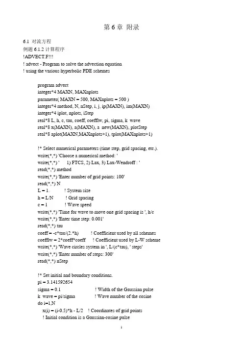
第6章附录6.1 对流方程例题6.1.2计算程序!ADVECT.F!!!! advect - Program to solve the advection equation! using the various hyperbolic PDE schemesprogram advectinteger*4 MAXN, MAXnplotsparameter( MAXN = 500, MAXnplots = 500 )integer*4 method, N, nStep, i, j, ip(MAXN), im(MAXN)integer*4 iplot, nplots, iStepreal*8 L, h, c, tau, coeff, coefflw, pi, sigma, k_wavereal*8 x(MAXN), a(MAXN), a_new(MAXN), plotStepreal*8 aplot(MAXN,MAXnplots+1), tplot(MAXnplots+1)!* Select numerical parameters (time step, grid spacing, etc.).write(*,*) 'Choose a numerical method: 'write(*,*) ' 1) FTCS, 2) Lax, 3) Lax-Wendroff : 'read(*,*) methodwrite(*,*) 'Enter number of grid points: 100'read(*,*) NL = 1. ! System sizeh = L/N ! Grid spacingc = 1 ! Wave speedwrite(*,*) 'Time for wave to move one grid spacing is ', h/cwrite(*,*) 'Enter time step: 0.001'read(*,*) taucoeff = -c*tau/(2.*h) ! Coefficient used by all schemescoefflw = 2*coeff*coeff ! Coefficient used by L-W schemewrite(*,*) 'Wave circles system in ', L/(c*tau), ' steps'write(*,*) 'Enter number of steps: 300'read(*,*) nStep!* Set initial and boundary conditions.pi = 3.141592654sigma = 0.1 ! Width of the Gaussian pulsek_wave = pi/sigma ! Wave number of the cosinedo i=1,Nx(i) = (i-0.5)*h - L/2 ! Coordinates of grid pointsa(i) = cos(k_wave*x(i)) * exp(-x(i)**2/(2*sigma**2))enddo! Use periodic boundary conditionsdo i=2,(N-1)ip(i) = i+1 ! ip(i) = i+1 with periodic b.c.im(i) = i-1 ! im(i) = i-1 with periodic b.c.enddoip(1) = 2ip(N) = 1im(1) = Nim(N) = N-1!* Initialize plotting variables.iplot = 1 ! Plot counternplots = 50 ! Desired number of plotsplotStep = float(nStep)/nplotstplot(1) = 0 ! Record the initial time (t=0)do i=1,Naplot(i,1) = a(i) ! Record the initial stateenddo!* Loop over desired number of steps.do iStep=1,nStep!* Compute new values of wave amplitude using FTCS,! Lax or Lax-Wendroff method.if( method .eq. 1 ) then !!! FTCS method !!!do i=1,Na_new(i) = a(i) + coeff*( a(ip(i))-a(im(i)) )enddoelse if( method .eq. 2 ) then !!! Lax method !!!do i=1,Na_new(i) = 0.5*( a(ip(i))+a(im(i)) ) +& coeff*( a(ip(i))-a(im(i)) )enddoelse !!! Lax-Wendroff method !!!do i=1,Na_new(i) = a(i) + coeff*( a(ip(i))-a(im(i)) ) +& coefflw*( a(ip(i))+a(im(i))-2*a(i) ) enddoendifa(i) = a_new(i) ! Reset with new amplitude valuesenddo!* Periodically record a(t) for plotting.if( (iStep-int(iStep/plotStep)*plotStep) .lt. 1 ) theniplot = iplot+1tplot(iplot) = tau*iStepdo i=1,Naplot(i,iplot) = a(i) ! Record a(i) for plotingenddowrite(*,*) iStep, ' out of ', nStep, ' steps completed'endifenddonplots = iplot ! Actual number of plots recorded!* Print out the plotting variables: x, a, tplot, aplotopen(11,file='x.txt',status='unknown')open(12,file='a.txt',status='unknown')open(13,file='tplot.txt',status='unknown')open(14,file='aplot.txt',status='unknown')do i=1,Nwrite(11,*) x(i)write(12,*) a(i)do j=1,(nplots-1)write(14,1001) aplot(i,j)enddowrite(14,*) aplot(i,nplots)enddodo i=1,nplotswrite(13,*) tplot(i)enddo1001 format(e12.6,', ',$) ! The $ suppresses the carriage return stopend!***** To plot in MATLAB; use the script below ******************** !load x.txt; load a.txt; load tplot.txt; load aplot.txt;!%* Plot the initial and final states.!figure(1); clf; % Clear figure 1 window and bring forward!plot(x,aplot(:,1),'-',x,a,'--');!legend('Initial','Final');!pause(1); % Pause 1 second between plots!%* Plot the wave amplitude versus position and time!figure(2); clf; % Clear figure 2 window and bring forward!mesh(tplot,x,aplot);!ylabel('Position'); xlabel('Time'); zlabel('Amplitude');!view([-70 50]); % Better view from this angle!****************************************************************** ================================================6.2 抛物形方程例题6.2.2计算程序!!!!dftcs.f!!!!!!!!!!! dftcs - Program to solve the diffusion equation! using the Forward Time Centered Space (FTCS) scheme.program dftcsinteger*4 MAXN, MAXnplotsparameter( MAXN = 300, MAXnplots = 500 )integer*4 N, i, j, iplot, nStep, plot_step, nplots, iStepreal*8 tau, L, h, kappa, coeff, tt(MAXN), tt_new(MAXN)real*8 xplot(MAXN), tplot(MAXnplots), ttplot(MAXN,MAXnplots)!* Initialize parameters (time step, grid spacing, etc.).write(*,*) 'Enter time step: 0.0001'read(*,*) tauwrite(*,*) 'Enter the number of grid points: 50 'read(*,*) NL = 1. ! The system extends from x=-L/2 to x=L/2h = L/(N-1) ! Grid sizekappa = 1. ! Diffusion coefficientcoeff = kappa*tau/h**2if( coeff .lt. 0.5 ) thenwrite(*,*) 'Solution is expected to be stable'elsewrite(*,*) 'WARNING: Solution is expected to be unstable'endif!* Set initial and boundary conditions.do i=1,Ntt(i) = 0.0 ! Initialize temperature to zero at all pointstt_new(i) = 0.0enddo!! The boundary conditions are tt(1) = tt(N) = 0!! End points are unchanged during iteration!* Set up loop and plot variables.iplot = 1 ! Counter used to count plotsnStep = 300 ! Maximum number of iterationsplot_step = 6 ! Number of time steps between plots nplots = nStep/plot_step + 1 ! Number of snapshots (plots)do i=1,Nxplot(i) = (i-1)*h - L/2 ! Record the x scale for plotsenddo!* Loop over the desired number of time steps.do iStep=1,nStep!* Compute new temperature using FTCS scheme.do i=2,(N-1)tt_new(i) = tt(i) + coeff*(tt(i+1) + tt(i-1) - 2*tt(i))enddodo i=2,(N-1)tt(i) = tt_new(i) ! Reset temperature to new valuesenddo!* Periodically record temperature for plotting.if( mod(iStep,plot_step) .lt. 1 ) then ! Every plot_step stepsdo i=1,N ! record tt(i) for plottingttplot(i,iplot) = tt(i)enddotplot(iplot) = iStep*tau ! Record time for plotsiplot = iplot+1endifenddonplots = iplot-1 ! Number of plots actually recorded!* Print out the plotting variables: tplot, xplot, ttplotopen(11,file='tplot.txt',status='unknown')open(12,file='xplot.txt',status='unknown')open(13,file='ttplot.txt',status='unknown')do i=1,nplotswrite(11,*) tplot(i)enddowrite(12,*) xplot(i)do j=1,(nplots-1)write(13,1001) ttplot(i,j)enddowrite(13,*) ttplot(i,nplots)enddo1001 format(e12.6,', ',$) ! The $ suppresses the carriage returnstopend!***** To plot in MATLAB; use the script below ********************!load tplot.txt; load xplot.txt; load ttplot.txt;!%* Plot temperature versus x and t as wire-mesh and contour plots.!figure(1); clf;!mesh(tplot,xplot,ttplot); % Wire-mesh surface plot!xlabel('Time'); ylabel('x'); zlabel('T(x,t)');!title('Diffusion of a delta spike');!pause(1);!figure(2); clf;!contourLevels = 0:0.5:10; contourLabels = 0:5;!cs = contour(tplot,xplot,ttplot,contourLevels); % Contour plot!clabel(cs,contourLabels); % Add labels to selected contour levels!xlabel('Time'); ylabel('x');!title('Temperature contour plot');!******************************************************************! program diffu_explicit.for! explicit methods for finite diffrencedimension T(51,51)real dx,dt,lamda,kp,Tmax,Tminopen(2,file='diffu_1.dat')dx=0.5dt=0.1kp=0.835lamda=kp*dt/dx/dxTmax=100.Tmin=0.imax=21write(*,*) 'lamda=',lamdado i=1,50do j=1,50T(i,j)=0.0do j=1,40T(1,j)=TmaxT(imax,j)=Tminend dodo j=1,40do i=2,20T(i,j+1)=T(i,j)+lamda*(T(i+1,j)-2.*T(i,j)+T(i-1,j)) end dowrite(2,222) (T(i,j),i=1,21)end do222 format(1x,21(2x,f18.10))end% diffu_explicit.mclc; clear all;nl = 20.; nt = 40;dx = 0.5; dt = 0.1; kp = 0.835;lamda = kp*dt/dx/dx;Tl = 0.; Tr = 100.;T = zeros(nl,nt);T(1,:) = Tl; T(nl,:)=Tr;for j=1:nt-1for i =2:nl-1T(i,j+1)=T(i,j)+lamda*(T(i+1,j)-2.*T(i,j)+T(i-1,j));endendsurf(T');xlabel('x');ylabel('time');zlabel('Temperature');title('explicit scheme');! diffu_implicit.for! implicit methods for finite diffrenceexternal tridparameter (imax=21,kmax=50)dimension t(imax),a(imax),b(imax),c(imax),r(imax),u(imax) real dx,dt,lamda,kp,tmax,tminopen(2,file='diffu_2.dat')dx=0.5lamda=kp*dt/dx/dxtmax=100.tmin=0.write(*,*) 'lamda=',lamdado i=2,imax-1! t(i)=tmax-(tmax-tmin)/(imax-1.)*(i-1.) t(i)=0.0end dot(1)=tmaxt(imax)=tmin! write(*,*) a(i),b(i),c(i)b(1)=1.c(1)=0.r(1)=t(1)a(imax)=0.b(imax)=1.r(imax)=t(imax)do i=2,imax-1a(i)=-lamdab(i)=1.+2.*lamdac(i)=-lamdar(i)=t(i)end dok=01 k=k+1call trid(a,b,c,r,u,imax)do i=1,imaxt(i)=u(i)r(i)=u(i)end dowrite(2,222) (t(i),i=1,imax)! write(*,222) (t(i),i=1,imax)if(k.lt.kmax) goto 1222 format(1x,21(2x,f18.12))endsubroutine trid(a,b,c,r,u,n)parameter (nmax=100)real gam(nmax),a(n),b(n),c(n),u(n),r(n)if (b(1)==0.) pause 'b(1)=0 in trid'bet=b(1)u(1)=r(1)/betdo j=2,ngam(j)=c(j-1)/betbet=b(j)-a(j)*gam(j)if (bet==0.) pause 'bet=0 in trid'u(j)=(r(j)-a(j)*u(j-1))/betend dodo j=n-1,1,-1u(j)=u(j)-gam(j+1)*u(j+1)end doend subroutine trid================================================== 6.3椭圆方程例题6.3.1计算程序! program overrelaxation.for! overrelaxation_iteration_methods for finite diffrence! of the 2d_Laplacian difference equationparameter(imax=25,jmax=25,pi=3.1415926)dimension T(imax,jmax),a(imax,jmax),& qx(imax,jmax),qy(imax,jmax),q(imax,jmax),an(imax,jmax) real lamda,Tu,Td,Tl,Tr,kpx,kpy,dx,dyopen(2,file='overrelaxation.dat')open(3,file='q.dat')lamda=1.5;Tu=100.;Tl=75.;Tr=50.;Td=0.;dx=1.;dy=1.;kmax=9 kpx=-0.49/2./dx;kpy=-0.49/2./dydo i=1,imaxdo j=1,jmaxT(i,j)=0.0end doend doT(1,1)=0.5*(Td+Tl) ;T(1,jmax)=0.5*(Tl+Tu)T(imax,jmax)=0.5*(Tu+Tr);T(imax,1)=0.5*(Tr+Td)do j=2,jmax-1T(1,j)=Tl; T(imax,j)=Trend dodo i=2, imax-1T(i,1)=Td; T(i,jmax)=Tuend dok=0do i=2,imax-1do j=2,jmax-1a(i,j)=T(i,j)T(i,j)=0.25*(T(i+1,j)+T(i-1,j)+T(i,j+1)+T(i,j-1))T(i,j)=lamda*T(i,j)+(1.-lamda)*a(i,j)end doend doep=abs((T(2,2)-a(2,2))/T(2,2))if(k.lt.kmax) goto 5write(*,*) 'ep=',epdo j=1,jmaxwrite(2,222) (T(i,j),i=1,imax)end do222 format(1x,25(2x,f14.10))do i=2,imax-1do j=2,jmax-1qx(i,j)=kpx*(T(i+1,j)-T(i-1,j))qy(i,j)=kpy*(T(i,j+1)-T(i,j-1))q(i,j)=sqrt(qx(i,j)*qx(i,j)+qy(i,j)*qy(i,j))if(qx(i,j).gt.0.) thenan(i,j)=atan(qy(i,j)/qx(i,j))elsean(i,j)=atan(qy(i,j)/qx(i,j))+piend ifend doend dodo j=2,jmax-1do i=2,imax-1! write(3,333) dx*(i-1),dy*(j-1),an(i,j),q(i,j)write(3,333) dx*(i-1),dy*(j-1),qx(i,j),qy(i,j)end doend do333 format(1x,4(2x,f18.12))End================================================= 例题6.3.2计算程序!!!!xadi.f90!!!!!program xadiuse AVDefuse DFLibparameter(n=19)real aj(n),bj(n),cj(n)integer statusreal T(0:n,0:n),TT(0:n,0:n)real lamda,Tu,Td,Tl,Tr,dx,dy,dt,kaopen(2,file='T3.dat')Tu=100.;Tl=75.;Tr=50.;Td=0.;dx=1.;dy=1.;kmax=10;dt=1.ka=0.835; lamda=ka*dt/(dx*dx)write(*,*) 'lamda=',lamdaT = 0.T(0,:) = Tl; T(n,:) =TrT(:,0) = Td; T(:,n) =TuT(0,0)=0.5*(Td+Tl);T(0,n)=0.5*(Tl+Tu)T(n,n)=0.5*(Tu+Tr);T(n,0)=0.5*(Tr+Td)! 系数矩阵赋值aj(:)=-lamda; ai(:)=lamdabj(:)= 2.*(1.+lamda); bi(:)=2.*(1-lamda)cj(:)=-lamda; ci(:)=lamdacall faglStartWatch(T, status)! 相当于随时间演化do k=1,kmaxdo i=1,n-1do j=1,n-1r(j)=ai(i)*T(i-1,j)+bi(i)*T(i,j)+ci(i)*T(i+1,j)end dor(1)=r(1)-aj(1)*T(i,0)r(n-1)=r(n-1)-cj(n-1)*T(i,n)call tridag(aj,bj,cj,r,u,n-1)do j=1,n-1T(i,j)=u(j)end doend do! 将矩阵T转置计算x方向call reverse(n,T,TT)do i=1,n-1do j=1,n-1r(j)=ai(i)*TT(i-1,j)+bi(i)*TT(i,j)+ci(i)*TT(i+1,j) end dor(1)=r(1)-aj(1)*TT(i,0)r(n-1)=r(n-1)-cj(n-1)*TT(i,n)call tridag(aj,bj,cj,r,u,n-1)do j=1,n-1TT(i,j)=u(j)end doend docall reverse(n,TT,T)call faglUpdate(T, status)call faglShow(T, status)end dopausecall faglClose(T, status)call faglEndWatch(T, status)do j=0,nwrite(2,222) (T(i,j),i=0,n)end do222 format(1x,20(2x,f14.10))endSUBROUTINE tridag(a,b,c,r,u,n)INTEGER n,NMAXREAL a(n),b(n),c(n),r(n),u(n)PARAMETER (NMAX=500)INTEGER jREAL bet,gam(NMAX)if(b(1).eq.0.)pause 'tridag: rewrite equations'bet=b(1)u(1)=r(1)/betdo 11 j=2,ngam(j)=c(j-1)/betbet=b(j)-a(j)*gam(j)if(bet.eq.0.)pause 'tridag failed'u(j)=(r(j)-a(j)*u(j-1))/bet11 continuedo 12 j=n-1,1,-1u(j)=u(j)-gam(j+1)*u(j+1)12 continuereturnENDSUBROUTINE REVERSE(n,T,TT) integer n,i,jreal T(0:n,0:n),TT(0:n,0:n)do i=0,ndo j=0,nTT(i,j)=T(j,i)end doend doreturnend================================================6.4 非线性偏微分方程% gasdynamincs_lw_1.mclc; clear all;xmin=-1.; xmax=1.; nx=101; h=(xmax-xmin)/(nx-1);r=0.9; cad=0.; time=0.; gamma=1.4; bcl=1.; bcr=1.;fprintf(' Space step - %f \n',h); fprintf(' \n');dd(1:nx)=zeros(1,nx); ud(1:nx)=zeros(1,nx); pd(1:nx)=zeros(1,nx);x(1:nx)=xmin+((1:nx)-1)*h;% Test 1te=' ( Test 1 )';rol=1.; ul=0.; pl=1.;ror=0.125; ur=0.; pr=0.1;tp=5.5;% Test 3%te=' ( Test 3 )';%rol=0.1; ul=0.; pl=1.;%ror=1.; ur=0.; pr=100.;%tp=0.05;% Initial conditionsdd(1:(nx-1)/2+1)=rol; ud(1:(nx-1)/2+1)=ul; pd(1:(nx-1)/2+1)=pl;dd((nx-1)/2+2:nx)=ror;ud((nx-1)/2+2:nx)=ur; pd((nx-1)/2+2:nx)=pr;[d,u,p,e,time]=lw_gasdynamics(dd,ud,pd,h,nx,r,cad,tp,gamma,bcl,bcr);% Exact solutionfor n=1:nx[density, velocity, pressure]=riemann(x(n),time,rol,ul,pl,ror,ur,pr,gamma);de(n)=density; ue(n)=velocity; pe(n)=pressure;ee(n)=pressure/((gamma-1.)*density);endfigure(1);plot(x,de,'k-',x,d,'k--');xlabel(' x ');ylabel(' density ');title([' Example 6.1 ',te]);figure(2);plot(x,ue,'k-',x,u,'k--');xlabel(' x ');ylabel(' velocity ');title([' Example 6.1 ',te]);figure(3);plot(x,pe,'k-',x,p,'k--');xlabel(' x ');ylabel(' pressure ');title([' Example 6.1 ',te]);figure(4);plot(x,ee,'k-',x,e,'k--');xlabel(' x ');ylabel(' internal energy ');title([' Example 6.1 ',te]);clear all;% Lax-Wendroff scheme (gasdynamics)function [d,u,p,e,time]=lw_gasdynamics(dd,ud,pd,h,nx,r,cad,tp,gamma,bcl,bcr)sd(1,1:nx)=dd(1:nx);sd(2,1:nx)=dd(1:nx).*ud(1:nx);sd(3,1:nx)=pd(1:nx)/(gamma-1.)+0.5*(dd(1:nx).*ud(1:nx)).*ud(1:nx);si(1:3,1:nx+1)=zeros(3,nx+1); av(1:3,1:nx)=zeros(3,nx);time=0.;while time <= tpsta=max(abs(sd(2,:)./sd(1,:))+...sqrt(gamma*(gamma-1)*(sd(3,:)./sd(1,:)-0.5*(sd(2,:).*sd(2,:))./(sd(1,:).*sd(1,:)))));tau=r*h*sqrt(1.-2.*cad)/sta;time=time+tau; %fprintf(' time - %f \n',time);% first stepif bcl == 0sl1=sd(1,2); sl2=-sd(2,2); sl3=sd(3,2);elsesl1=sd(1,2); sl2=sd(2,2); sl3=sd(3,2);endgl(1)=sl2;gl(2)=(gamma-1.)*sl3+0.5*(3.-gamma)*sl2^2/sl1;gl(3)=sl2*(gamma*sl3-0.5*(gamma-1.)*sl2^2/sl1)/sl1;for n=1:nxif (n == 1)|(n == nx)av(:,n)=[ 0.; 0.; 0.;];elseav(:,n)=cad*(sd(:,n+1)-2.*sd(:,n)+sd(:,n-1));endsr1=sd(1,n); sr2=sd(2,n); sr3=sd(3,n);gr(1)=sr2;gr(2)=(gamma-1.)*sr3+0.5*(3.-gamma)*sr2^2/sr1;gr(3)=sr2*(gamma*sr3-0.5*(gamma-1.)*sr2^2/sr1)/sr1;si(1,n)=0.5*(sl1+sr1)-(gr(1)-gl(1))*tau*0.5/h;si(2,n)=0.5*(sl2+sr2)-(gr(2)-gl(2))*tau*0.5/h;si(3,n)=0.5*(sl3+sr3)-(gr(3)-gl(3))*tau*0.5/h;gl(:)=gr(:);sl1=sr1; sl2=sr2; sl3=sr3;endif bcr == 0sr1=sd(1,nx-1); sr2=-sd(2,nx-1); sr3=sd(3,nx-1);elsesr1=sd(1,nx-1); sr2=sd(2,nx-1); sr3=sd(3,nx-1);endgr(1)=sr2;gr(2)=(gamma-1.)*sr3+0.5*(3.-gamma)*sr2^2/sr1;gr(3)=sr2*(gamma*sr3-0.5*(gamma-1.)*sr2^2/sr1)/sr1;si(1,nx+1)=0.5*(sl1+sr1)-(gr(1)-gl(1))*tau*0.5/h;si(2,nx+1)=0.5*(sl2+sr2)-(gr(2)-gl(2))*tau*0.5/h;si(3,nx+1)=0.5*(sl3+sr3)-(gr(3)-gl(3))*tau*0.5/h;% second stepfl(1)=si(2,1);fl(2)=(gamma-1.)*si(3,1)+0.5*(3.-gamma)*si(2,1)^2/si(1,1);fl(3)=si(2,1)*(gamma*si(3,1)-0.5*(gamma-1.)*si(2,1)^2/si(1,1))/si(1,1);for n=2:nx+1fr(1)=si(2,n);fr(2)=(gamma-1.)*si(3,n)+0.5*(3.-gamma)*si(2,n)^2/si(1,n);fr(3)=si(2,n)*(gamma*si(3,n)-0.5*(gamma-1.)*si(2,n)^2/si(1,n))/si(1,n);su(:,n-1)=sd(:,n-1)-(fr(:)-fl(:))*tau/h+av(:,n-1);fl(:)=fr(:);endsd(:,1:nx)=su(:,1:nx);endd(1:nx)=su(1,1:nx); u(1:nx)=su(2,1:nx)./su(1,1:nx);p(1:nx)=(gamma-1.)*(su(3,1:nx)-0.5*(su(2,1:nx).*su(2,1:nx))./su(1,1:nx));e(1:nx)=(su(3,1:nx)-0.5*(su(2,1:nx).*su(2,1:nx))./su(1,1:nx))./su(1,1:nx);return;% Solves Riemann problem for ideal gas% r1, u1, p1 initial parameters for x<0% r2, u2, p2 initial parameters for x>0% rf, uf, pf solution at the point (x,t)% c1, c2 sound speeds for x<0 and for x>0% s1, sr velocties of the fronts of S(hock)W(ave)s% shl, shr velocties of the fronts of the heads of R(arefaction)Ws% stl, str velocties of the tails of RWsfunction [rf,uf,pf]=riemann(x,t,r1,u1,p1,r2,u2,p2,gamma)g(1)=0.5*(gamma-1.)/gamma; g(2)=0.5*(gamma+1.)/gamma; g(3)=2.*gamma/(gamma-1.); g(4)=2./(gamma-1.); g(5)=2./(gamma+1.); g(6)=(gamma-1.)/(gamma+1.);g(7)=0.5*(gamma-1.); g(8)=1./gamma; g(9)=gamma-1.;s=x/t;c1 = sqrt(p1/(r1*g(8)));c2 = sqrt(p2/(r2*g(8)));du=u2-u1;% Vacuum solutionuvac=g(4)*(c1+c2)-du;if uvac <= 0.disp(' Vacuum generated by given data');return;end% Apply Newton method% Initial guessespv=0.5*(p1+p2)-0.125*du*(r1+r2)*(c1+c2);pmin=min(p1,p2); pmax=max(p1,p2); qrat=pmax/pmin;if ( qrat <= 2. ) & ( pmin <= pv & pv <= pmax )p=max(1.0e-6,pv);elseif pv < pminpnu=c1+c2-g(7)*du;pde=c1/(p1^g(1))+c2/(p2^g(1));p=(pnu/pde)^g(3);elsegel=sqrt((g(5)/r1)/(g(6)*p1+max(1.0e-6,pv)));ger=sqrt((g(5)/r2)/(g(6)*p2+max(1.0e-6,pv)));p=(gel*p1+ger*p2-du)/(gel+ger); p=max(1.0e-6,p);endendp0=p; err=1.;while err > 1.0e-5if p <= p1prat=p/p1; fl=g(4)*c1*(prat^g(1)-1.); ffl=1./(r1*c1*prat^g(2));elsea=g(5)/r1; b=g(6)*p1; qrt=sqrt(a/(b+p));fl=(p-p1)*qrt; ffl=(1.-0.5*(p-p1)/(b+p))*qrt;endif p <= p2prat=p/p2; fr=g(4)*c2*(prat^g(1)-1.); ffr=1./(r2*c2*prat^g(2));elsea=g(5)/r2; b=g(6)*p2; qrt=sqrt(a/(b+p));fr=(p-p2)*qrt; ffr=(1.-0.5*(p-p2)/(b+p))*qrt;endp=p-(fl+fr+du)/(ffl+ffr);err=2.*abs(p-p0)/(p+p0); p0=p;endif p0 < 0.p0=1.0e-6;end% Velocity of CDu0=0.5*(u1+u2+fr-fl);if s <= u0if p0 <= p1shl=u1-c1;if s <= shlrf=r1; uf=u1; pf=p1; return;elsecml=c1*(p0/p1)^g(1); stl=u0-cml;if s > stlrf=r1*(p0/p1)^g(8); uf=u0; pf=p0; return;elseuf=g(5)*(c1+g(7)*u1+s); c=g(5)*(c1+g(7)*(u1-s));rf=r1*(c/c1)^g(4); pf=p1*(c/c1)^g(3);return;endendelsepml=p0/p1; sl=u1-c1*sqrt(g(2)*pml+g(1));if s <= slrf=r1; uf=u1; pf=p1; return;elserf=r1*(pml+g(6))/(pml*g(6)+1.); uf=u0; pf=p0; return;endendelseif p0 > p2pmr=p0/p2; sr=u2+c2*sqrt(g(2)*pmr+g(1));if s >= srrf=r2; uf=u2; pf=p2; return;elserf=r2*(pmr+g(6))/(pmr*g(6)+1.); uf=u0; pf=p0; return;endelseshr=u2+c2;if s >= shrrf=r2; uf=u2; pf=p2; return;elsecmr=c2*(p0/p2)^g(1); str=u0+cmr;if s <= strrf=r2*(p0/p2)^g(8); uf=u0; pf=p0; return;elseuf=g(5)*(-c2+g(7)*u2+s); c=g(5)*(c2-g(7)*(u2-s));rf=r2*(c/c2)^g(4); pf=p2*(c/c2)^g(3);return;endendendendreturn;%%%%%%%%% gasdynamics_Godunov.m%%%%%%%%%%%%%clc; clear all;xmin=-1.; xmax=1.; nx=101; h=(xmax-xmin)/(nx-1);r=0.9; gamma=1.4; bcl=1.; bcr=1.;fprintf('gasdynamics_godunov \n'); fprintf(' Space step - %f \n',h); fprintf(' \n'); dd(1:nx-1)=zeros(1,nx-1); ud(1:nx-1)=zeros(1,nx-1); pd(1:nx-1)=zeros(1,nx-1);x(1:nx)=xmin+((1:nx)-1)*h; xa=xmin+((1:nx-1)-0.5)*h;% Test 1te=' ( Test 1 )';rol=1.; ul=0.; pl=1.;ror=0.125; ur=0.; pr=0.1;tp=15.5;% Test 2%te=' ( Test 2 )';%rol=1.; ul=0.; pl=1000.;%ror=1.; ur=0.; pr=1.;%tp=0.024;% Test 3%te=' ( Test 3 )';%rol=0.1; ul=0.; pl=1.;%ror=1.; ur=0.; pr=100.;%tp=0.05;% Test 4%te=' ( Test 4 )';%rol=5.99924; ul=19.5975; pl=460.894;%ror=5.99242; ur=-6.19633; pr=46.0950;%tp=0.05;% Test 5%te=' ( Test 5 )';%rol=3.86; ul=-0.81; pl=10.33;%ror=1.; ur=-3.44; pr=1.;%tp=0.5;% Initial conditionsdd(1:(nx-1)/2)=rol; ud(1:(nx-1)/2)=ul; pd(1:(nx-1)/2)=pl;dd((nx-1)/2+1:nx-1)=ror;ud((nx-1)/2+1:nx-1)=ur; pd((nx-1)/2+1:nx-1)=pr;[d,u,p,e,time]=godunov_gasdynamics(dd,ud,pd,h,nx,r,tp,gamma,bcl,bcr);% Exact solutionfor n=1:nx[density, velocity, pressure]=riemann(x(n),time,rol,ul,pl,ror,ur,pr,gamma);de(n)=density; ue(n)=velocity; pe(n)=pressure;ee(n)=pressure/((gamma-1.)*density);endfigure(1);plot(x,de,'k-',xa,d,'ko');xlabel(' x ');ylabel(' density ');title([' Example 6.3 ',te]);figure(2);plot(x,ue,'k-',xa,u,'ko');xlabel(' x ');ylabel(' velocity ');figure(3);plot(x,pe,'k-',xa,p,'ko');xlabel(' x ');ylabel(' pressure ');figure(4);plot(x,ee,'k-',xa,e,'ko');xlabel(' x ');ylabel(' internal energy ');clear all;% Method of S. K. Godunovfunction [d,u,p,e,time]=godunov_gasdynamics(dd,ud,pd,h,nx,r,tp,gamma,bcl,bcr)g(1)=0.5*(gamma-1.)/gamma; g(2)=0.5*(gamma+1.)/gamma; g(3)=2.*gamma/(gamma-1.); g(4)=2./(gamma-1.); g(5)=2./(gamma+1.); g(6)=(gamma-1.)/(gamma+1.);g(7)=0.5*(gamma-1.); g(8)=1./gamma; g(9)=gamma-1.;sd(1,1:nx-1)=dd(1:nx-1);sd(2,1:nx-1)=dd(1:nx-1).*ud(1:nx-1);sd(3,1:nx-1)=pd(1:nx-1)/(gamma-1.)+0.5*(dd(1:nx-1).*ud(1:nx-1)).*ud(1:nx-1);time=0.;while time <= tpsta=max(abs(sd(2,:)./sd(1,:))+...sqrt(gamma*(gamma-1)*(sd(3,:)./sd(1,:)-0.5*(sd(2,:).*sd(2,:))./(sd(1,:).*sd(1,:)))));tau=r*h/sta;time=time+tau; %fprintf(' %f \n',time);if bcl == 0[f1,f2,f3]=flux_godunov(sd(1,1),-sd(2,1),sd(3,1),sd(1,1),sd(2,1),sd(3,1),g(:));else[f1,f2,f3]=flux_godunov(sd(1,1),sd(2,1),sd(3,1),sd(1,1),sd(2,1),sd(3,1),g(:));endfleft(1)=f1; fleft(2)=f2; fleft(3)=f3;for n=1:nx-2[f1,f2,f3]=flux_godunov(sd(1,n),sd(2,n),sd(3,n),sd(1,n+1),sd(2,n+1),sd(3,n+1),g(:));fright(1)=f1; fright(2)=f2; fright(3)=f3;su(:,n)=sd(:,n)-(fright(:)-fleft(:))*tau/h;fleft(:)=fright(:);endif bcr == 0[f1,f2,f3]=flux_godunov(sd(1,nx-1),sd(2,nx-1),sd(3,nx-1),sd(1,nx-1),-sd(2,nx-1),...sd(3,nx-1),g(:));else[f1,f2,f3]=flux_godunov(sd(1,nx-1),sd(2,nx-1),sd(3,nx-1),sd(1,nx-1),sd(2,nx-1),...sd(3,nx-1),g(:));endfright(1)=f1; fright(2)=f2; fright(3)=f3;su(:,nx-1)=sd(:,nx-1)-(fright(:)-fleft(:))*tau/h;sd(:,1:nx-1)=su(:,1:nx-1);endd(1:nx-1)=su(1,1:nx-1); u(1:nx-1)=su(2,1:nx-1)./su(1,1:nx-1);p(1:nx-1)=(gamma-1.)*(su(3,1:nx-1)-0.5*(su(2,1:nx-1).*su(2,1:nx-1))./su(1,1:nx-1));e(1:nx-1)=(su(3,1:nx-1)-0.5*(su(2,1:nx-1).*su(2,1:nx-1))./su(1,1:nx-1))./su(1,1:nx-1); return;% Solves Riemann problem for ideal gas% r1, u1, p1 initial parameters for x<0% r2, u2, p2 initial parameters for x>0% rf, uf, pf solution at the point (x,t)% c1, c2 sound speeds for x<0 and for x>0% s1, sr velocties of the fronts of S(hock)W(ave)s% shl, shr velocties of the fronts of the heads of R(arefaction)Ws% stl, str velocties of the tails of RWsfunction [rf,uf,pf]=riemann(x,t,r1,u1,p1,r2,u2,p2,gamma)g(1)=0.5*(gamma-1.)/gamma; g(2)=0.5*(gamma+1.)/gamma; g(3)=2.*gamma/(gamma-1.);g(7)=0.5*(gamma-1.); g(8)=1./gamma; g(9)=gamma-1.;s=x/t;c1 = sqrt(p1/(r1*g(8)));c2 = sqrt(p2/(r2*g(8)));du=u2-u1;% Vacuum solutionuvac=g(4)*(c1+c2)-du;if uvac <= 0.disp(' Vacuum generated by given data');return;end% Apply Newton method% Initial guessespv=0.5*(p1+p2)-0.125*du*(r1+r2)*(c1+c2);pmin=min(p1,p2); pmax=max(p1,p2); qrat=pmax/pmin;if ( qrat <= 2. ) & ( pmin <= pv & pv <= pmax )p=max(1.0e-6,pv);elseif pv < pminpnu=c1+c2-g(7)*du;pde=c1/(p1^g(1))+c2/(p2^g(1));p=(pnu/pde)^g(3);elsegel=sqrt((g(5)/r1)/(g(6)*p1+max(1.0e-6,pv)));ger=sqrt((g(5)/r2)/(g(6)*p2+max(1.0e-6,pv)));p=(gel*p1+ger*p2-du)/(gel+ger); p=max(1.0e-6,p);endendp0=p; err=1.;while err > 1.0e-5if p <= p1prat=p/p1; fl=g(4)*c1*(prat^g(1)-1.); ffl=1./(r1*c1*prat^g(2));elsea=g(5)/r1; b=g(6)*p1; qrt=sqrt(a/(b+p));fl=(p-p1)*qrt; ffl=(1.-0.5*(p-p1)/(b+p))*qrt;endif p <= p2prat=p/p2; fr=g(4)*c2*(prat^g(1)-1.); ffr=1./(r2*c2*prat^g(2));a=g(5)/r2; b=g(6)*p2; qrt=sqrt(a/(b+p));fr=(p-p2)*qrt; ffr=(1.-0.5*(p-p2)/(b+p))*qrt;endp=p-(fl+fr+du)/(ffl+ffr);err=2.*abs(p-p0)/(p+p0); p0=p;endif p0 < 0.p0=1.0e-6;end% Velocity of CDu0=0.5*(u1+u2+fr-fl);if s <= u0if p0 <= p1shl=u1-c1;if s <= shlrf=r1; uf=u1; pf=p1; return;elsecml=c1*(p0/p1)^g(1); stl=u0-cml;if s > stlrf=r1*(p0/p1)^g(8); uf=u0; pf=p0; return;elseuf=g(5)*(c1+g(7)*u1+s); c=g(5)*(c1+g(7)*(u1-s));rf=r1*(c/c1)^g(4); pf=p1*(c/c1)^g(3);return;endendelsepml=p0/p1; sl=u1-c1*sqrt(g(2)*pml+g(1));if s <= slrf=r1; uf=u1; pf=p1; return;elserf=r1*(pml+g(6))/(pml*g(6)+1.); uf=u0; pf=p0; return;endendelseif p0 > p2pmr=p0/p2; sr=u2+c2*sqrt(g(2)*pmr+g(1));if s >= srrf=r2; uf=u2; pf=p2; return;rf=r2*(pmr+g(6))/(pmr*g(6)+1.); uf=u0; pf=p0; return;endelseshr=u2+c2;if s >= shrrf=r2; uf=u2; pf=p2; return;elsecmr=c2*(p0/p2)^g(1); str=u0+cmr;if s <= strrf=r2*(p0/p2)^g(8); uf=u0; pf=p0; return;elseuf=g(5)*(-c2+g(7)*u2+s); c=g(5)*(c2-g(7)*(u2-s));rf=r2*(c/c2)^g(4); pf=p2*(c/c2)^g(3);return;endendendendreturn;% Solves Riemann problem and computes fluxes for method of S. K. Godunov% r1, u1, p1 parameters in left cell% r2, u2, p2 parameters in right cell% rf, uf, pf parameters on the interface% c1, c2 sound speeds in left and right cells% s1, sr velocties of the fronts of S(hock)W(ave)s% shl, shr velocties of the fronts of the heads of R(arefaction)Ws% stl, str velocties of the tails of RWsfunction [f1,f2,f3]=flux_godunov(sl1,sl2,sl3,sr1,sr2,sr3,g)r1=sl1; u1=sl2/r1; p1=(1./g(8)-1.)*(sl3-0.5*sl2*u1);r2=sr1; u2=sr2/r2; p2=(1./g(8)-1.)*(sr3-0.5*sr2*u2);% sound speeds in left and right cellsc1 = sqrt(p1/(r1*g(8)));c2 = sqrt(p2/(r2*g(8)));du=u2-u1;% Vacuum solution。
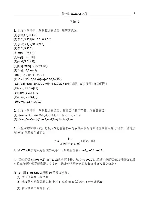
习题 11. 执行下列指令,观察其运算结果, 理解其意义: (1) [1 2;3 4]+10-2i(2) [1 2; 3 4].*[0.1 0.2; 0.3 0.4] (3) [1 2; 3 4].\[20 10;9 2] (4) [1 2; 3 4].^2 (5) exp([1 2; 3 4]) (6)log([1 10 100]) (7)prod([1 2;3 4])(8)[a,b]=min([10 20;30 40]) (9)abs([1 2;3 4]-pi)(10) [1 2;3 4]>=[4,3;2 1](11)find([10 20;30 40]>=[40,30;20 10])(12) [a,b]=find([10 20;30 40]>=[40,30;20 10]) (提示:a 为行号,b 为列号) (13) all([1 2;3 4]>1) (14) any([1 2;3 4]>1) (15) linspace(3,4,5) (16) A=[1 2;3 4];A(:,2)2. 执行下列指令,观察其运算结果、变量类型和字节数,理解其意义: (1) clear; a=1,b=num2str(a),c=a>0, a= =b, a= =c, b= =c (2) clear; fun='abs(x)',x=-2,eval(fun),double(fun)3. 本金K 以每年n 次,每次p %的增值率(n 与p 的乘积为每年增值额的百分比)增加,当增加到rK 时所花费的时间为)01.01ln(ln p n rT +=(单位:年)用MA TLAB 表达式写出该公式并用下列数据计算:r =2, p =0.5, n =12.4.已知函数f (x )=x 4-2x 在(-2, 2)内有两个根。
取步长h =0.05, 通过计算函数值求得函数的最小值点和两个根的近似解。

matlab讲义随机过程实验讲义刘继成华中科技大学数学与统计学院前言 (1)第一章Matlab 简介 (2)第二章简单分布的模拟 (6)第三章基本随机过程 (9)第四章Markov过程 (12)第五章模拟的应用和例子 (16)附录各章的原程序 (51)参考文献 (75)若想检验数学模型是否反映客观现实,最自然的方法是比较由模型计算的理论概率和由客观试验得到的经验频率。
不幸的是,这两件事都往往是费时的、昂贵的、困难的,甚至是不可能的。
此时,计算机模拟在这两方面都可以派上用场:提供理论概率的数值估计与接近现实试验的模拟。
模拟的第一步自然是在计算机程序的算法中如何产生随机性。
程序语言,甚至计算器,都提供了“随机”生成[0,1]区间内连续数的方法。
因为每次运行程序常常生成相同的“随机数”,因此这些数被称为伪随机数。
尽管如此,对于多数的具体问题这样的随机数已经够用。
我们将假定计算机已经能够生成[0,1]上的均匀随机数。
也假定这些数是独立同分布的,尽管它们常常是周期的、相关的、……。
……本讲义的安排如下,第一章是Matlab简介,从实践动手角度了解并熟悉Matlab环境、命令、帮助等,这将方便于Matlab的初学者。
第二章是简单随机变量的模拟,只给出了常用的Matlab 模拟语句,没有堆砌同一种变量的多种模拟方法。
对于没有列举的随机变量的模拟,以及有特殊需求的读者应该由这些方法得到启发,或者参考更详细的其他文献资料。
第三章是基本随机过程的模拟。
主要是简单独立增量过程的模拟,多维的推广是直接的。
第四章是Markov过程的模拟。
包括服务系统,生灭过程、简单分支过程等。
第五章是这些模拟的应用。
例如,计算概率、估计积分、模拟现实、误差估计,以及减小方差技术,特别给读者提供了一些经典问题的模拟,通过这些问题的模拟将会更加牢固地掌握实际模拟的步骤。
平稳过程的模拟、以及利用平稳过程来预测的内容并没有包含在本讲义之内,但这丝毫不影响该内容的重要性,这也是将会增补进来的主要内容之一。