
NMR软件——MestReNova介绍简介
- 格式:ppt
- 大小:1.54 MB
- 文档页数:29


在MestReNova软件中,可以通过以下步骤进行溶剂峰的定标:
1.打开需要定标的核磁数据文件。
选择一般为fid,打开方式中选择MestReNova。
2.在打开的文件界面中,选择需要进行定标的区域。
通常首先观察芳香区,也就是化
学位移在7左右的区域。
3.在软件界面中,找到红框中的键,对溶剂峰进行定标。
选择7.26附近的峰,将ppm
值改为7.26。
4.如果需要手动设置阈值,可以通过“标峰-手动设置阈值”进行设置,将不需要的杂质
峰滤掉。
5.如果需要进行溶剂峰化学位移纠正,可以通过“分析-参考-参考(R)”进行操作。
6.一般情况下,在标准溶剂峰化学位移位置附近寻找最高的峰,将其化学位移修改为
正确的值,然后点击OK即可完成溶剂峰化学位移纠正。
7.最后,可以通过“分析-积分-自动检测区域”得出需要的大部分信息。


核磁数据处理方法核磁共振(NMR)是一种重要的分析技术,广泛应用于化学、生物医学等领域。
在核磁实验中,我们通常需要对得到的数据进行处理和分析,以获得有关样品的结构和性质信息。
本文将详细介绍核磁数据处理的常用方法和步骤。
一、数据预处理1. 原始数据导入:将核磁实验得到的原始数据导入到数据处理软件中,例如Bruker TopSpin、MestReNova等。
2. 数据校正:根据实验条件和仪器参数,对原始数据进行校正,包括频率校正、相位校正等,以确保数据的准确性和可靠性。
3. 噪声滤波:对数据进行噪声滤波处理,以减少噪声对后续分析的影响。
二、数据处理1. 傅里叶变换:对原始数据进行傅里叶变换,将时域数据转换为频域数据,以便进行进一步的分析。
2. 谱线拟合:对傅里叶变换后的频域数据进行谱线拟合,以确定峰的位置、强度和宽度等参数。
3. 化学位移校正:根据已知参考物质的化学位移值,对样品的化学位移进行校正,以获得准确的化学位移数据。
4. 积分峰面积:对谱线进行积分,计算峰的面积,以获得样品中各组分的相对含量。
5. 噪声去除:对数据进行噪声去除处理,以提高信噪比,减少噪声对分析结果的干扰。
6. 数据平滑:对数据进行平滑处理,以减少峰的峰宽,提高峰的分辨率。
三、数据分析1. 化学结构判断:根据化学位移数据和已知的化学结构信息,判断样品中各组分的化学结构。
2. 定量分析:根据峰的面积和已知参考物质的浓度,进行定量分析,计算样品中各组分的绝对含量。
3. 动力学分析:根据数据的时间序列信息,进行动力学分析,研究反应速率、反应机理等。
4. 结构优化:根据实验数据,进行份子结构的优化,以获得最稳定的构象和最低的能量。
四、结果解释和报告撰写1. 结果解释:根据数据处理和分析结果,解释样品的结构和性质信息,提出合理的解释和判断。
2. 报告撰写:根据实验目的和要求,撰写核磁数据处理的报告,包括实验原理、方法、结果和讨论等内容。
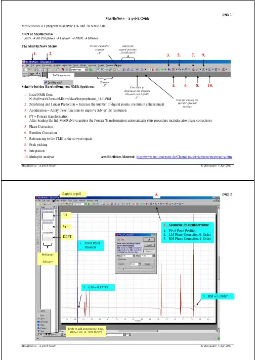
page 1 MestReNova – A quick Guide MestReNova is a program to analyze 1D- and 2D NMR data. Start of MestReNova Start All Programs The MestReNova MenuChemieNMRMNovaCreate expanded regions „E“ Adjust the signal intensity „Scrollwheel“1.2.3.5.7.9.Pulldownmenu Zoomen „Z“Schritte bei der Bearbeitung von NMR-Spektren:1. Load NMR Data N:\Software\Chemie\MNova\data\butyrophenon_1h.fid\fidCrosshair to determine the distance between two signals „C“4.6.8.10.2. Zerofilling and Linear Prediction = Increase the number of digital points, resolution enhancement 3. Apodization = Apply these functions to improve S/N or the resolutionTool for cutting out specific spectral regions4. FT = Fourier transformation After loading the fid, MestReNova applies the Fourier Transformation automatically (this procedure includes also phase correction). 5. Phase Correction 6. Baseline Correction 7. Referencing to the TMS or the solvent signal 8. Peak picking 9. Integration 10. Multiplet analysisMestReNova – A quick GuideAusführliches Manual: http://www.uni-muenster.de/Chemie.oc/service/nmr/mestrenova.htmK. Bergander, 5-Apr-2011Export to pdf5.page 21H 5. Manuelle Phasenkorrektur 1. Pivot Point Position 2. LM Phase Correction 0. Order 3. RM Phase Correction 1. Order 1. Pivot Point Position für die Phasen13CDEPTMultipage Software2. LM = 0.Order 3. RM = 1.OrderTools to add annotations, lines, arrows, etc. to your spectraMestReNova – A quick GuideK. Bergander, 5-Apr-2011page 3 NMR data processing with MestReNova The structure of the MestReNova program is comparable to Powerpoint. So, you can create for each spectrum a separate page: 1H-, 13C-, gCOSY- and gHSQC. After loading the raw data (FID file), the data will be processed (FT, phase correction) automatically. Unfortunately the automatic phase correction doesn’t work properly all the time, thus sometimes it’s necessary to redo the phase correction manually. After you’ve finished the processing, save these data as MNova file. In this way, you will be able to reload these data later, without the necessity to redo the processing. Start the Program•StartAll ProgramsChemieNMRMNova1. Load data• • •Strg O Choose the right fid/ser-file Fourier Transformation and Phase Correction are executed automatically, so that the transformed spectrum will appear after loading the fid. Processing After it, the signal shape will be smoothed.2. Zero Filling and Linear Prediction• •Generally, the data points of the raw data (Spectrum Size) are doubled by zero fillingLinear Prediction is an algorithm to calculate the expected data points at the zero filled end of the FID (forward prediction). The alternative backward prediction is primarily used for nuclei with extreme short T1-values to calculate the beginning of the FID. In this way the problem of baseline distortions (due to probe ringing) is solved.3. Apodization a) Improvement of Signal to Noise (S/N), e.g. in case of 13C NMR spectra The exponential multiplication emphasizes the beginning of the FID (signal), whereas the end of the FID (noise) is weighted less. In this way the S/N ratio is improved, but at the cost of getting broader lines (linebroadening). The bigger the lb value is, the broader appears the resulting line. Typical lb values for 13C: Exponential lb = + 1 Hz. Improvement of Resolution, e.g. in case of 1H spectra to resolve small line splitting The Gaussian multiplication emphasizes the end of the FID’s (coupling and noise), whereas the beginning of the FID (signal) is weighted less. The resolution of the signal will be improved on the cost of a worse signal to noise ratio. Typical values for 1H: Gaussian = 0.1 to 0.5, Exponential: lb= - 0.1 to – 1.0b)MestReNova – A quick GuideK. Bergander, 5-Apr-2011page 4 4. FT = Fourier transformation•The Fourier transformation is executed automatically after opening the fid file.5. Phase correction• •Chose the option Manual Correction within the pull-down menu Phase Correction. The procedure of phase correction is described in detail on the screenshot on the next page. Bear in mind that the automatic phase correction leads quite often to poor results.6. Baseline correction• •Select the option Baseline Correction within the pull-down menu Baseline Correction. Then select the Whittaker Smoother as method. From now on the method Whittaker Smoother is used during the Full Auto baseline correction.7. Reference the TMS or the solvent signal• • •Click on the TMS button. Place the appearing red cursor line to the signal which should be referenced and click the LM. Either you enter the corresponding ppm value manually, or you select the corresponding solvent after clicking the Solvents button.8. Peak-Picking• • •Select the option manual threshold within the pull-down menu Peak Picking. Press the LM left to the signal, hold the LM and drag the cursor over the signal. The appearing horizontal line defines the lowest intensity of all signals which should be labeled with peak picking.9. Integration• • •Select the option Manual within the pull-down menu Integration. Press the LM left to the signal, hold the LM and drag the cursor over the signal. To normalize an integral value, place the cursor to the integral and click the LM two times. Enter the right integral value in the appearing window (e.g. 3 for a single CH3 group).MestReNova – A quick GuideK. Bergander, 5-Apr-2011page 5 10. ZoomenExpandFull Zoom out Enter the limits manually11. Vertical Scale•The easiest way to adjust the vertical scale is done with the scroll wheel.Scale the most intense signal to the height of pageDecrease signal intensity Increase signal intensity erhöhen12. Crosshair to determine line splitting• • • •It appears an info-box and a blue cursor line. Move the blue cursor line to the left signal of the multiplet. Press the LM, hold the LM and move the additional appearing line to the next signal. The info-box will display the line splitting in Hz.13. Stack two or more spectra on one page (e.g. 13C and DEPT)• • • •1st page: Load 13C spectrum (fid) 2nd page: Load DEPT Mark both pages on the left by using the Strg-key + the LM ( Menu bar on the top: Stack Stack Spectrablue border)MestReNova – A quick GuideK. Bergander, 5-Apr-2011page 6 14.•Processing of „stacked“ spectra left menu barAutomatic vertical scale Invert the order of stacked spectra Select spectra for processing13C is activated for processing, so during phase correction only the phase of the carbon spectrum is changed, but not the phase of the dept spectra.15.• • •New Cut function With the aid of this function you can suppress the display of certain spectral regions (e.g. regions, which show no signal). Select the button which shows a signal & scissors on the top menu bar. Move the appearing cursor left to the region which you like to suppress, press and hold the LM and drag the mouse over the region to suppress. Copy/Paste into other Windows programs (Word, Powerpoint)• •16.Click with the LM inside the spectrum, so that a green border will appear around the specified spectrum. Now you can copy the specified spectrum from MNova to e.g. Word by using Ctrl C and Ctrl V. Create spectral expansions on the top of the page17.• • •Click on the button spectrum & glasses, so that the cursor appears as magnifier and a plus sign. Press the LM left to the signal, hold the LM and drag the cursor over the region, which should be expanded. If you like, you can process the expanded region after activating this expanded region by clicking the LM inside the expanded region.MestReNova – A quick GuideK. Bergander, 5-Apr-2011page 7 18.• • •Predict NMR Spectra Draw your structure with ChemDraw and copy and paste this structure on a new page in MNova. 13 Menu bar on the top: Predict C Spectrum. If you move the cursor to a carbon of the structure the corresponding carbon signal will be highlighted by a blue line.If you move the cursor on a specific signal the corresponding carbon of the structure will be highlighted by a red box.blue cursorMestReNova – A quick GuideK. Bergander, 5-Apr-2011page 8 19. • • • • • • • • • Shortcuts Strg C / Strg V Strg O Strg M Strg Z Z C E Hold Space bar Esc : Copy/Paste e.g. to copy a structure from ChemDraw to a page of MNova or to copy a spectrum from MNova to Word. : Open NMR data : New page : Undo the last action : Select the Zoom mode : Select the Crosshair mode : Select the Expand mode : While you’re holding the space bar, the panning mode is selected temporarily. So you can move the displayed spectral region. : Leave the last chosen modeMestReNova – A quick GuideK. Bergander, 5-Apr-2011page 9 20.• • • • •2D spectra with external projections (see screenshot on the next page) 1st page : Load 1H spectrum (fid) 2nd page : Load 13C spectrum (fid) 3rd page : Load gHSQC spectrum (fid oder ser) Left menu bar: Select the pull-down menu Show Traces (Icon with 2D-Plot + projections) and select Setup. Select the right 1H and 13C projections and define them as vertical and horizontal projection (cp. screenshot). Phase correction of phase sensitive 2D NMR Spectra (1J(C,H) correlation = gHSQC)•21.Phase sensitive 2D spectra need a phase correction along the F2 (1H) and the F1 (13C) axis. The main principle of 2D phase correction is comparable to that one for 1D phase correction. The only difference is that you have to choose the direction which should be adjusted (F1 or F2) by clicking on the corresponding F1 or F2 button.MestReNova – A quick GuideK. Bergander, 5-Apr-20112.2D NMR: 1J(C,H)-Korrelation 1. Load ghsqc/fid 2. Select Show Traces 3. Setup 4. Select H for the horizontal trace 5. Select C for the vertical tracepage 103. 4. 5.MestReNova – A quick GuideK. Bergander, 5-Apr-2011page 11 Right phase along F1 und F2: Positive absorption signal in F1 and F2 e.g. CH3 or CH in gHSQC Negative absorption signal in F1 and F2 e.g. diastereotopic CH2 in gHSQCPhase error along F2: Dispersion signal Positive and negative parts along F2Phase error along F1: Dispersion signal along F1 Positive and negative parts along F1Phase error along F1 and F2: Dispersion signal along F1and F2 Positive and negative parts along F1 and F2MestReNova – A quick GuideK. Bergander, 5-Apr-2011page 12 21. MNova by using a Terminalserver If you want to run Mnova from your personal PC at home it’s necessary to install the CISCO client (for details see the next section). After connecting the WWU network by vpn you will be able to start the terminal server on nwzhome.uni-muenster.de. To have access to local saved data, check the option Allow acces to your local disk drives within the pull-down menu Options>>! Start → All Programs → Accessories → Remote Desktop Connectionusername: 22. • • •nwzhome.uni-muenster.de\your nwznet accountInstallation des VPN CISCO Clients First of all, you need to define your Netzzugangspasswort on the internet site Mein ZIV. https://www.uni-muenster.de/ZIV/MeinZIV/index.html Enter https://www.uni-muenster.de/ZIVwiki/bin/view/Anleitungen/CiscoIPSecVPNSetup into your browser download: a) Installationsanleitung des Cisco-VPN-Client für Windows b) The appropriate VPN-client software for your system c) The vpn-standard-profil: vpnstandard.pcf•Install the client software corresponding to the manual a). Define the following exception for the vpn server vpnserver.uni-muenster.de and vpnserver2.uni-muenster.de: UDP-Port 500, IP-Protocol 50 (ESP)Firewall :23. • •Start of the VPN connection Start the Cisco program. Establish the vpn connection by using the “standard.pcf” profile and by entering your account and your “Netzzugangspasswort”.K. Bergander, 5-Apr-2011MestReNova – A quick Guide。