Distributions of discriminants of cubic algebras
- 格式:pdf
- 大小:521.37 KB
- 文档页数:37


Cumulative dominance and probabilistic sophistication*Rakesh Sarin a, Peter P. Wakker ba The Anderson Graduate School of Management, UCLA, Los Angeles, CAb CentER, Tilburg University, Tilburg, The NetherlandsDecember 1998AbstractMachina and Schmeidler gave preference conditions for probabilistic sophistication, i.e., decision making where uncertainty can be expressed in terms of (subjective) probabilities without commitment to expected utility maximization. This note shows that simpler and more general results can be obtained by combining results from qualitative probability theory with a "cumulative dominance" axiom.Keywords: Probabilistic sophistication; Subjective probability; Qualitative probability Corresponding author:Peter WakkerCentER for Economic ResearchTilburg UniversityP.O. Box 90153Tilburg, 5000 LE, The Netherlands--31-13-466.24.57 (O)--31-13-466.32.80 (F)--31-13-466.23.40 (S)*****************.LeidenUniv.NL* The support for this research was provided in part by the Decision, Risk, and Management Science branch of the National Science Foundation.Machina & Schmeidler (1992) pose an interesting question: What conditions on an agent's preferences justify probabilistic sophistication; that is, when can beliefs be represented by probabilities? A probabilistically sophisticated agent may deviate from expected utility in his preferences over lotteries but must express uncertainty in terms of additive probabilities. In this note, we show that a cumulative dominance condition can be used to simplify and extend the results of Machina & Schmeidler (1992). In a previous paper (Sarin & Wakker 1992), we showed that cumulative dominance is a necessary condition for Choquet expected utility, and it can be used to extend expected utility under risk to Schmeidler's (1989) Choquet expected utility under uncertainty. It turns out that cumulative dominance is necessary for probabilistic sophistication as well, and here we show that this axiom can be used to extend qualitative probability for two-consequence acts to probabilistically sophisticated preferences for many-consequence acts.Let S denote the state space; is the algebra of subsets of S, the elements of which are called events; is the set of consequences; is the set of acts, i.e., maps from S to that are finite-valued and measurable (f-1(x)∈ for all consequences x); x denotes both a consequence and the related constant act. By u we denote the preference relation over acts, that also denotes the induced ordering of consequences. The notation s (strict preference), ~ (equivalence), e, and c is as usual. In this note, probability measures are finitely additive and need not be countably additive unless stated otherwise.Following Machina & Schmeidler (1992), an agent is probabilistically sophisticated if there exists a probability measure P over S such that:(i)The agent chooses between acts based on the probability distributions generatedover the consequences.(ii)First-order stochastic dominance is satisfied.Stochastic dominance in (ii) is taken in the strict sense (see Machina & Schmeidler 1992, Section 3.1). It relates to general, possibly nonmonetary, outcomes, and is defined as follows: f s g whenever P(f u x) ≥ P(g u x) for all consequences x with strict inequality for at least one x. We have modified the definition of probabilistic sophistication of Machina & Schmeidler by omitting their "mixture continuity" condition, in order to allow for general models with atoms (e.g., in Theorem 5 below). Machina & Schmeidler show that mixture continuity is implied by Savage's P6, hence it can be seen to be implied in our Theorem 2.We next derive a more likely than relation on events from preferences between two-consequence acts. We write A uλB if there exist consequences x s y such that the act [x if A; y if not A] is preferred to the act [x if B; y if not B]. Obviously, probabilistic sophistication requires that A uλB if and only if P(A)≥P(B), i.e., P is an agreeing probability measure for uλ. For the case where contains only two consequences, one immediately observes that probabilistic sophistication holds if and only if an agreeing probability measure exists. Machina & Schmeidler (1992, Section 3.4) demonstrate that the existence of an agreeing probability measure need not imply probabilistic sophistication when there are more than two consequences. To obtain probabilistic sophistication for general acts, Machina & Schmeidler assume the restrictions of Savage's axioms that guarantee the existence of a probability measure agreeing with uλ, and then add an additional axiom (P4* in their paper) for acts with many consequences.We will follow the first part of their analysis but use cumulative dominance instead of their P4* to ensure probabilistic sophistication. In line with the strict stochastic dominance condition of Machina & Schmeidler, we strengthen the definition of cumulative dominance of Sarin & Wakker (1992) somewhat and define a strict version thereof. Cumulative dominance holds iff ug whenever {s∈S: f(s)u x} uλ {s∈S: g(s)u x} for all consequences x,where the preference between f and g is strict whenever one of the antecedentuλ orderings is strict (sλ).This condition says that if one considers the cumulative event [x or more] more likely under f than under g for every consequence x, then f should be preferred to g, where the more likely than relation uλ is derived from choices. The following elementary lemma shows the way in which cumulative dominance ensures probabilistic sophistication for many-consequence acts in situations where an agreeing probability measure exists for uλ.Lemma 1. The following two statements are equivalent.(i)Probabilistic sophistication holds.(ii)There exists an agreeing probability measure P for uλ and cumulative dominance holds.Proof. If a probability measure P agrees with uλ and if preferences depend only on probability distributions generated over consequences through P, then one immediately sees that cumulative dominance and stochastic dominance are equivalent. So we only have to show:•Under (i), P agrees with uλ: This is elementarily verified.•Under (ii), preferences depend only on probability distributions generated over consequences: If f and g generate the same probability distribution overconsequences, then {s∈S: f(s)u x} ~λ {s∈S: g(s)u x} for all consequences x, and hence f u g and f u g, by twofold application of cumulative dominance. That is, f~ g.∼Preference characterizations of probabilistic sophistication can be derived from the above lemma by substituting preference conditions, obtained from qualitative probability theory, to guarantee the existence of an agreeing probability measure P foruλ. Several such conditions have been presented in qualitative probability theory. Hence, our approach shows a way to derive probabilistic sophistication from results of qualitative probability theory. As a first illustration, we invoke the qualitative probability conditions of Savage (1954); for definitions the reader is referred to Savage (1954) or Machina & Schmeidler (1992). We assume their P1 (weak ordering), P3 (tastes are independent of beliefs), P4 (beliefs are independent of tastes), P5 (nontriviality), and P6 (fineness of the state space); P7 is not needed because we only consider finite-valued acts. We note that P4 need not be stated because it is implied by cumulative dominance (see the proof below), and restrict P2 to two-consequence acts:Postulate P2* (sure-thing principle for two-consequence acts). For all consequences x s y and events A,B,H with A∩H = B∩H = ∅:[x if A; y if not A]u[x if B; y if not B]if and only if[x if A∪H; y if not A∪H] u[x if B∪H; y if not B∪H]Theorem 2. Assume Savage's (1954) P1, P3, P5, and P6. Then the following two statements are equivalent.(i)Probabilistic sophistication holds.(ii)P2* and cumulative dominance hold.Proof. It is obvious that (i) implies (ii), therefore we assume (ii) and derive (i). P4 follows from the restriction of cumulative dominance to two-consequence acts. P1,P2*, P3, P4, P5, and P6 are all that Savage needs to derive an agreeing probability measure. His analysis, as well as that of Machina & Schmeidler (1992), assumes that is the collection of all subsets of S. It is well-known that these proofs and results immediately extend to any sigma-algebra of events (Savage 1954, Section III.4; Machina & Schmeidler 1992, Section 6.2). Our theorem extends the result further to any algebra of events: Savage's axioms P1, P2*, P3, P4, P5, and P6 also imply theexistence of an agreeing probability measure for that case (Wakker 1981). Now the theorem follows from Lemma 1. ∼Machina & Schmeidler (1992) eloquently pose the question what additional conditions are needed to characterize probabilistic sophistication over many-consequence acts once an agreeing probability measure exists for uλ. Once one assumes qualitative probability theory, then our characterization seems to be the simplest way to obtain probabilistic sophistication in the Savage framework. Note here that qualitative probability theory is the special case of additive conjoint measurement with two-element component sets (Fishburn & Roberts 1988).For many results of probability theory, countable additivity of a probability measure is essential. Hence Machina & Schmeidler (1992, Section 6.2) address the characterization of countable additivity in probabilistic sophistication. They conjecture that conditions of Villegas (1964) and Arrow (1965) may be used to imply countable additivity. We prove that that is indeed the case. Following Villegas (1964), monotone continuity holds if for each sequence of events A j that increases to an event A (A j+1⊃A j and ∪A j = A), A j eλB for all j implies A eλB. In the presence of this condition, Savage's structural condition P6 can be weakened to the requirement that no atoms exist. An event A is an atom if it is nonnull but it cannot be partitioned into two nonnull events.Theorem 3. Assume Savage's (1954) P1, P3, and P5, assume that is a sigma algebra, and that there are no atoms. Then the following two statements are equivalent.(i)Probabilistic sophistication holds with respect to a countably additive probabilitymeasure.(ii)P2*, monotone continuity, and cumulative dominance hold.Proof. The implication (i) ⇒ (ii) is straightforward, hence we assume (ii) and derive (i). Cumulative dominance implies P4. P4 in turn implies weak ordering of uλ(i.e.,Villegas 1964, Conditions Q1(a), Q1(b), and Q1(c)). Now, mainly because of P3 and P5, it follows that ∅cλS and, for any event A, ∅eλA eλS (Villegas' ConditionQ1(d)). P2* implies Villegas' condition Q2 for uλ. Now, by Theorem 4.3 of Villegas, there exists a unique countably additive probability measure agreeing with uλ. By our Lemma 1, Statement (i) holds. ∼By means of the above result, it can be demonstrated that the conjecture in Section 6.2 of Machina & Schmeidler (1992) is correct.Corollary 4. In Theorem 2 of Machina & Schmeidler (1992), the probability measure in (ii) is countably additive if in Statement (i) their monotone continuity axiom is added, and the domain of events is assumed a sigma algebra.Proof. Monotone continuity as defined here and in Villegas (1964) follows from the first part of the monotone continuity axiom of Machina & Schmeidler (1992, Section6.2) by defining, for outcomes x c y, f = [y if A, x if A c], E j = A\A j, and g = [y if B, x ifB c]. Their preference conditions imply probabilistic sophistication and hence, by Lemma 1, cumulative dominance. Also there exist no atoms in their model, mainly by P6. Now the result follows from Lemma 1 and Theorem 3. ∼Finally, we give an example of an alternative derivation of probabilistic sophistication using a qualitative probability result different than that of Savage. We invoke the remarkable result provided by Chateauneuf (1985). Chateauneuf provided necessary and sufficient conditions for the existence of an agreeing probability measure in full generality, i.e., without assuming any restrictive condition such as Savage's P6 or nonatomicity. His result extends the earlier results by Kraft, Pratt, & Seidenberg (1959) and Scott (1964), who gave necessary and sufficient conditions for finite state spaces. For brevity, we do not describe the details of these conditions, but refer the reader to the respective papers. Extensions were provided by Lehrer (1991).Theorem 5 (general probabilistic sophistication). The following two statements are equivalent.(i)Probabilistic sophistication holds.(ii)Cumulative dominance holds, and Chateauneuf's (1985) conditions hold for uλ. Proof. See Chateauneuf (1985) and Lemma 1. ∼By means of Chateauneuf's conditions and our Lemma 1, we thus obtain a characterization of probabilistic sophistication in full generality. The above result can be extended to the case where in (i) the probability measure is countably additive. Obviously, many alternative derivations of probabilistic sophistication can be obtained by applying Lemma 1 to other results of qualitative probability theory. For instance, Zhang (1998) shows how to extend results to domains more general than algebras. Fishburn (1986) gives an extensive survey of such results. An alternative approach, using the model of Anscombe and Aumann (1963), is presented by Machina & Schmeidler (1995).A possible objection to our result may be that cumulative dominance is too close to the functional form it seeks to characterize and therefore the proof is trivial. We note, however, that the purpose of characterizations is to provide preference conditions that are simple to understand and that can be directly tested through observable choices. The focus should be on the insights that preference conditions generate and not on the complexity of proofs they entail. The condition of Machina & Schmeidler (1992) is a generalization of independence of beliefs from tastes and in that manner it provides new insights. Our cumulative dominance condition is an extension of stochastic dominance to the case of uncertainty and thus it reveals the nature of probabilistic sophistication in a transparent and empirically meaningful way.ReferencesAnscombe, F.J. & Robert J. Aumann (1963), "A Definition of Subjective Probability,"Annals of Mathematical Statistics 34, 199−205.Arrow, Kenneth J. (1965), "Aspects of the Theory of Risk-Bearing." Academic Bookstore, Helsinki. Elaborated as Kenneth J. Arrow (1971), "Essays in the Theory of Risk-Bearing." North-Holland, Amsterdam.Chateauneuf, Alain (1985), "On the Existence of a Probability Measure Compatible with a Total Preorder on a Boolean Algebra," Journal of Mathematical Economics 14, 43−52.Fishburn, Peter C. (1986), "The Axioms of Subjective Probability," Statistical Science 1, 335−358.Fishburn, Peter C. & Fred S. Roberts (1988), "Unique Finite Conjoint Measurement,"Mathematical Social Sciences 16, 107−143.Kraft, Charles H., John W. Pratt, & A. Seidenberg (1959), "Intuitive Probability on Finite Sets," Annals of Mathematical Statistics 30, 408−419.Lehrer, Ehud (1991), "On a Representation of a Relation by a Measure," Journal of Mathematical Economics 20, 107−118.Machina, Mark J. & David Schmeidler (1992), "A More Robust Definition of Subjective Probability," Econometrica 60, 745−780.Machina, Mark J. & David Schmeidler (1995), "Bayes without Bernoulli: Simple Conditions for Probabilistically Sophisticated Choice," Journal of Economic Theory 67, 106−128.Sarin, Rakesh K. & Peter P. Wakker (1992), "A Simple Axiomatization of Nonadditive Expected Utility," Econometrica 60, 1255-1272.Savage, Leonard J. (1954), "The Foundations of Statistics." Wiley, New York.(Second edition 1972, Dover, New York.)Schmeidler, David (1989), "Subjective Probability and Expected Utility without Additivity," Econometrica 57, 571-587.Scott, Dana (1964), "Measurement Structures and Linear Inequalities," Journal of Mathematical Psychology 1, 233-247.Villegas, C. (1964), "On Quantitative Probability σ-Algebras," Annals of Mathematical Statistics 35, 1787-1796.Wakker, Peter P. (1981), "Agreeing Probability Measures for Comparative ProbabilityStructures," The Annals of Statistics 9, 658-662.Zhang, Jiangkang (1998), "Qualitative Probabilities on Lambda-Systems,"Mathematical Social Sciences, forthcoming.。
Journal of Hazardous Materials132(2006)39–46Generation of urban road dust from anti-skid andasphalt concrete aggregatesHeikki Tervahattu a,b,∗,Kaarle J.Kupiainen b,Mika R¨a is¨a nen c,Timo M¨a kel¨a d,Risto Hillamo da Cooperative Institute for Research in Environmental Sciences,University of Colorado,Boulder,Campus Box216,CO80309,USAb Nordic Envicon Oy,Koetilantie3,FIN-00790Helsinki,Finlandc Department of Geology,University of Helsinki,P.O.Box64,FIN-00014Helsinki,Finlandd Finnish Meteorological Institute,Sahaajankatu20E,FIN-00810Helsinki,FinlandAvailable online19January2006AbstractRoad dust forms an important component of airborne particulate matter in urban areas.In many winter cities the use of anti-skid aggregates and studded tires enhance the generation of mineral particles.The abrasion particles dominate the PM10during springtime when the material deposited in snow is resuspended.This paper summarizes the results from three test series performed in a test facility to assess the factors that affect the generation of abrasion components of road dust.Concentrations,mass size distribution and composition of the particles were studied.Over90% of the particles were aluminosilicates from either anti-skid or asphalt concrete aggregates.Mineral particles were observed mainly in the PM10 fraction,thefine fraction being12%and submicron size being6%of PM10mass.The PM10concentrations increased as a function of the amount of anti-skid aggregate dispersed.The use of anti-skid aggregate increased substantially the amount of PM10originated from the asphalt concrete. It was concluded that anti-skid aggregate grains contribute to pavement wear.The particle size distribution of the anti-skid aggregates had great impact on PM10emissions which were additionally enhanced by studded tires,modal composition,and texture of anti-skid aggregates.The results emphasize the interaction of tires,anti-skid aggregate,and asphalt concrete pavement in the production of dust emissions.They all must be taken into account when measures to reduce road dust are considered.The winter maintenance and springtime cleaning must be performed properly with methods which are efficient in reducing PM10dust.©2005Elsevier B.V.All rights reserved.Keywords:Road dust;Mineral particles;PM10;SEM/EDX;Anti-skid and asphalt concrete aggregates;Paved roads;Studded tires;Hazardous dust;EU limit value1.IntroductionRoad dust has been acknowledged as a dominant source of PM10(particulate matter,aerodynamic diameter<10m)espe-cially during spring in many winter cities of Scandinavia,North America,and Japan and causes serious environmental prob-lems[1–5].Urban road dust is a complex mixture of particles released from several different sources.It is an important com-ponent of urban PM10and its composition is usually dominated by geological material[4,6–10].In addition to many kinds of discomfort,road dust causes negative health effects.Studies of exposure to mineral and resuspension particles have shown evi-dence of toxicity and a possibility of adverse health impacts ∗Corresponding author.Tel.:+135893866030;fax:+1358938694111.E-mail address:heikki.tervahattu@helsinki.fi(H.Tervahattu).[11–13].Respirable mineral particles,e.g.aluminosilicates and crystalline quartz,have been implicated in human diseases with lung cancer as most severe[14–16].Paved road dust is also a source of allergen exposure for the general population [17].The high proportion of road dust has been linked to the snowy winter conditions that makes it necessary to use trac-tion control methods.These measures enhance the generation of mineral particles.A fraction of the particles is deposited in snow and later released when the snow melts.These abra-sion particles are observed in high concentrations,especially during spring in urban areas with high volumes of traffic [4,18].The methods for traction control include dispersion of anti-skid aggregates on the road surface and equipping the tires with metal studs or a special rubber design.High particle concentra-tions have been connected in,e.g.Japan and Norway[1,2,19,20]0304-3894/$–see front matter©2005Elsevier B.V.All rights reserved. doi:10.1016/j.jhazmat.2005.11.08440H.Tervahattu et al./Journal of Hazardous Materials132(2006)39–46to the use of studded tires which also produce direct emissions from wearing of bare asphalt concrete.The use of anti-skid aggregates has also been linked to an increased particle loading in urban air[3,21,22].The formation processes of the particles are the mechanical wear of the actual anti-skid aggregate grains and the wear of asphalt pavement both by tires and by anti-skid aggregate particles[21].Urban road dust is an important issue also from the viewpoint of the European Union limit values for airborne particles(daily maximum for PM10is50g m−3,allowing35exceedances annually).This limit value is commonly exceeded in many Scandinavian cities due to springtime road dust.The Council Directive1999/30/EC allows member states to designate the zones within which the limit values are exceeded due to the resuspension of particulates following the winter sanding of roads.This statement challenges to study the impact of anti-skid aggregates on PM10concentrations.The aim of this work was to study experimentally the factors that affect the generation of abrasion components of road dust from the two mineral dust sources,asphalt concrete and anti-skid aggregates.This paper presents the main results from three test series.Some of the results are reported in[21,23,24].2.Experimental2.1.The test facility and aggregatesThis study was conducted in a test facility,which made it possible to rule out dust contributions from other sources than abrasion of asphalt concrete or anti-skid aggregates,and tires.The test room(180m3in volume)was cooled to a tem-perature of0–2◦C to represent the temperature in dry spring conditions.RH was50–75%.Two wheels were attached to an electrically powered rotating axel,with adjustable rotating speed.The axel system was tuned to move sideways so that the driving space of the tires becomes33cm.The diameter of the test ring was390cm.The tire pressure was2.0bar and the weight for each tire was300kg.The driving ring was sur-rounded with low walls to prevent the traction sand fromflyingoff.The impact of anti-skid aggregates on suspended PM(PM isused for all airborne particulate matter,since the concentrationsof total suspended particles[TSP]were measured)was studiedby using different amounts of sanding aggregates having vari-ous particle size distribution and different modal composition.It is difficult to estimate the shares of the different mineral dustsources,because they often have a similar mineralogical com-position[25].For these tests,aggregates(anti-skid and asphaltconcrete aggregates)with distinguishable mineralogy were cho-sen to be able to estimate the proportions from different dustsources.Tested asphalt concrete and anti-skid aggregates arealso used in real life.The modal compositions of tested aggre-gates are given in Table1.In tests during2001–2002only theasphalt concrete aggregate(mafic volcanic rock)contained themineral hornblende,which was used as a tracer for the min-eral dust from the asphalt concrete pavement.In2003tests theasphalt concrete aggregate was granite,and its minerals quartzand potassium feldspar were used as tracers because anti-skidaggregates did not contained these minerals.Three test seriesand a total of59tests were performed.Tests were performed with studded and friction tires toinvestigate asphalt concrete pavement wear and suspendedPM generation caused by different tires.Different amounts ofanti-skid aggregates were distributed(0,∼300,∼1000,and ∼2000g m−3)including four different natural anti-skid aggre-gates and blast furnace slag anti-skid aggregate.An amount oftraction sand was chosen to represent dirty road conditions foundin springtime when traction sand is accumulated on the pavementfor a long time.Two rock types were used as asphalt concreteaggregates to study the role of asphalt concrete aggregates in thePM generation.The impact of driving speed was studied usinglow speeds(either15or30km h−1).The results showed the fac-tors that affect the emissions as well as the relative importanceand the possible magnitude of the effect of these factors.Thefacility and the test descriptions are presented in more detail inKupiainen et al.[21,23,26]and R¨a is¨a nen et al.[24,27].Table1The modal compositions(%)of aggregatesAggregates Chemical formulaGranite1Granite2(Pernaja)Diabase Mafic volcanic rock(Patavuori)Sanding2001–2002Asphalt2003Sanding all tests Asphalt2001–2002,sanding2003Quartz30.428.4SiO2K-feldspar29.626.3KAlSi3O8Plagioclase32.439.457.429.4(Na,Ca)Al(Si,Al)Si2O8Biotite 5.9 1.8 3.8K(Mg,Fe)3(Al,Fe)Si3O10(OH,F)2 Hornblende53Ca2(Mg,Fe)4Al(Si7Al)O22(OH,F)2 Clinopyroxene17.3(Ca,Mg,Fe)2Si2O6(Augite) Olivine17.5(Mg,Fe)2SiO4Cummingtonite-grunerite12.8(Mg,Fe)7Si8O22(OH)2Others 1.7 4.14 4.8STT20.7 5.211.6 6.2LA10–14/4–5.642/4315/2416/2311/17Mafic volcanic rock was used as an asphalt concrete aggregate in2001–2002and as an anti-skid aggregate in2003.Granites were used as anti-skid aggregate in 2001–2002and as asphalt concrete aggregate in2003.STT:studded tire test value[30];LA10–14/4–5.6:Los Angeles test value for10–14/4–5.6mm[29].H.Tervahattu et al./Journal of Hazardous Materials132(2006)39–4641The particle size distribution of anti-skid aggregates was determined with sieves from0.063to8mm[28].The Los Ange-les test(LA)was used to determine aggregates’resistance to fragmentation[29]and it was performed from fractions10/14 to4/5.6mm,the latter according to Annex A with eight balls. The studded tire test(STT)measures the ability of an aggregate to tolerate the abrasive wear of studded tires[30].Point-counting method with a polarizing microscope was used to determine the modal composition of studied aggregates.The petrographical and mechanical-physical properties of the aggregates used in the tests are presented in more detail in Kupiainen et al.[21,23,26] and R¨a is¨a nen et al.[24,27].2.2.Particle sampling and analysisTwo high volume samplers(Wedding&Associates Sampler—TSP and PM10)were used to measure the concen-trations of suspended particles and to collect samples for the analyses of PM.In one test series the size distribution of the aerosol was studied and samples were collected for a more detailed PM research using two virtual impactors(VI—PM2.5–10 and PM2.5)and two12stage(0.045–10.7m)cascade impactors (SDI,[31]).The VIs were equipped with(Pallflex,type Tis-suquartz2500QAT-UP)quartz and(Millipore,type FS3-m) Polytetrafluoroethylene(PTFE)filters,the SDI with aluminium substrates and(Whatman,type Nuclepore800120)polycarbon-ate membranes and the high volume samplers with glassfiber filters(Munktell,type MG160).All inlets were situated simi-larly,approximately1.5m of the driving ring at a height of2.5m. After each test,the dust was allowed to settle for30–45min,and after that,the room was vacuumed and ventilated.Background concentration was monitored before the tests.The average back-ground was less than10%of the lowest concentration measured in the tests.The morphology,composition,and mineralogy of the parti-cles were determined from high volume TSP-and PM10-filters, and the cascade impactor membranes with individual parti-cle analysis by a scanning electron microscope(SEMZEISS DSM962)coupled with an energy dispersive X-ray analyzer (EDXLINK ISIS with ZAF-4measurement program).A sim-ilar instrumentation has been used in several particle studies [32–37].The analytical method is described in Kupiainen et al. [21,23].The morphology and chemistry offine and submicron parti-cles were studied in detail from the polycarbonate membranes of the cascade impactor.Afield emission SEM(FESEMJEOL JSM-6335F)coupled with an energy dispersive X-ray microan-alyzer(EDXLINK ISIS and INCA)was used for the analyses. Samples were prepared similarly as for conventional SEM,with Cr as the coating material.The acceleration voltage was15kV.The source contributions from asphalt concrete and sanding (in Figs.2,3and5)were estimated by comparing the abundance of minerals in the PM10samples with the mineralogy of the asphalt concrete and sanding materials[21,23].Comparison of five individual analyses from the same PM sample(studded tires, 1000g m−2of granite1)is shown in Kupiainen et al.[23].Based on that comparison the error for source contributions isestimated Fig.1.The correlation between PM10concentrations and the amount of anti-skid aggregate used in tests with the studded tires.The aggregate with lowest resistance against fragmentation(granite1,inside circles)caused higher emis-sions than aggregates having higher LA-values,especially with higher amounts of anti-skid aggregate.Mafic volcanic rock used as asphalt concrete aggregate. to be approximately12%.This error is indicated in Fig.3with error bars.The carbonaceous fractions,elemental carbon(EC),organic carbon(OC),and carbonate carbon,were determined from the VI-quartzfilter samples with a thermal–optical analyzer[38,39].3.Results3.1.Impacts of sanding on dust generationVery high increase in PM10concentrations was observed as a function of the amount of anti-skid aggregate dispersed on the asphalt concrete surface(Fig.1includes tests with studded tires). The concentrations were two fold with∼300g m−2of anti-skid aggregate,four fold with∼1000g m−2of anti-skid aggregate, and nine fold with2000g m−2compared with the experiments without the sanding.The dust concentrations correlated with the amount of anti-skid aggregate even though different sanding and asphalt concrete materials were used.The presented particle concentration data(Fig.1)would lead to conclude that the PM10dust originates mainly from sanding. This data does not,however,give any indication of the origin of the particles.The sources of the dust were investigated by an individual particle analysis studying the amount of particles originating from anti-skid and asphalt concrete aggregates.This was performed by measuring the fraction of different minerals in the PM10samples and comparing these fractions to the modal composition of the rocks(see Section2).Fig.2presents results from tests which show the impact of sanding on the modal composition of PM.Mafic volcanic rock was used as an asphalt concrete aggregate and granite as an anti-skid aggregate.Tests without anti-skid aggregates were used as a reference to show the mineral composition of PM from only asphalt concrete abrasion.Since all the hornblende must orig-inate from the asphalt concrete aggregate,its abundance was used as a basis to study the sources of the particles.Fig.2shows that when anti-skid aggregate was used,the share of hornblende decreased and shares of quartz and K-feldspar increased com-pared with the test without sand(asphalt-ref)indicating that dust was originated both from asphalt concrete and anti-skid42H.Tervahattu et al./Journal of Hazardous Materials132(2006)39–46Fig.2.The modal composition of PM10samples(studied by SEM/EDX); anti-skid-ref:the modal composition of the anti-skid aggregate(granite); sanding:the modal composition of dust sample PM10in the test with 1000g m−2of this anti-skid aggregate;asphalt-ref:the modal composition of dust sample PM10in the test without anti-skid aggregate(mafic volcanic rock as asphalt concrete aggregate). aggregates.This analysis of the dust by SEM/EDX showed that a large percentage of the particles(32–97%;70%on average, see[21])originated from the asphalt concrete.The use of anti-skid aggregates greatly increased the PM10 concentrations but the source of the particles in these experi-ments was predominantly from the asphalt concrete pavement. It was concluded from the analyses of the particle concentra-tions and of the particle chemistry that the anti-skid aggregate was not only crushed into small PM10particles but also increased the asphalt concrete wear.This phenomenon was named as“the sandpaper effect”.Kanzaki and Fukuda[40],and Lindgren[41] have previously suggested that loose particles(e.g.scraped off the road surface)may work as grinding material and increase the wear.Fig.3demonstrates the sandpaper effect.Two tests were performed without anti-skid aggregate.PM in these cases was generated only from asphalt concrete.The white line shows the maximum PM10concentration level of these tests.Anti-skid aggregate was used in all other tests.All the asphalt concrete-based PM above this line indicates PM generation by the sand-paper effect,which was a major source for suspended PM. 3.2.Impacts of asphalt concrete aggregatesThe granite anti-skid aggregates with different grain size dis-tribution was used to study the impact of the grading on the dust concentrations.The comparison of in tests(Fig.4)shows that high percentage offine-grained anti-skid aggregate particles of overall grading greatly increased the PM10concentrations when high amounts of sand were dispersed.This impact was observed both with studded and friction tires.PM from both the anti-skid aggregate and from asphalt concrete aggregate increased.When Fig.3.The fractions of PM10concentrations from the anti-skid aggregate(trac-tion sand)and from asphalt concrete as a function of increased sanding;mafic volcanic rock as asphalt concrete aggregate,granite1and diabase as anti-skid aggregates.Dark grey area represents PM10from asphalt concrete,light grey area from anti-skid aggregates.Tests1and2were performed without sanding. Sanding increased PM10from asphalt concrete:all PM10from asphalt concrete above the white line indicates the abrasive wear of the asphalt concrete by sand grains under the tires(the sandpaper effect).The error bars indicate the error of source contribution.there are morefine-grained particles the number and surface area of particles increase.Therefore,more particles can grind the asphalt concrete and the sandpaper effect increases.The properties of the rock used as anti-skid aggregates affected the PM10concentrations too.The aggregate with low-est resistance against fragmentation(granite1in Fig.1;LA value42/43,see Table1)caused higher emissions and the effect became more significant when more anti-skid aggregate was dis-persed.Diabase resulted in lower PM10concentrations but had a relatively large sandpaper effect.Fig.1showed that sanding greatly increased dust emission. These results were obtained in tests in which mafic volcanic rock was used as asphalt concrete aggregate.In order to study the impact of asphalt concrete aggregate on the generation of airborne PM,granite was used as asphalt concrete aggregate. Fig.5shows the comparison of PM10emissions using these two asphalt concretes and diabase anti-skid aggregate.Both rock aggregates have good mechanical properties[27].Great quanti-ties of PM10were measured in both cases but somewhat(20% on average)more when mafic volcanic rock(A1in Fig.1)was Fig.4.The impact of the grain size distribution of anti-skid aggregate on PM10 concentrations when different amounts of anti-skid aggregate(sand)were used. 1/5.6and2/5.6mm mean1–5.6and2–5.6mm sized grains.H.Tervahattu et al./Journal of Hazardous Materials132(2006)39–4643Fig.5.PM10concentrations generated from anti-skid and asphalt concrete aggregates.Two concretes and diabase as an anti-skid aggregate were used. Asphalt concrete was made out of mafic volcanic rock in A1(2001and2002) and of granite in A2(2003).Both traction and studded tires and different amounts of anti-skid aggregate(1000and2000g m−2)were used.used.The difference was statistically almost significant(Sign test,p=0.063,n=4).In order to know if there is any difference in the compo-sition of PM when different asphalt concrete aggregates were used,investigations were conducted on the shares of particles originated either from asphalt concrete aggregate or anti-skid aggregates using the same anti-skid material(diabase)and two different asphalt concrete aggregates.The results in Fig.5show that the share of PM from asphalt concrete aggregate was rela-tively lower when granite was used as asphalt concrete aggregate (A2in Fig.5).Because the total PM concentrations were also lower with granite,the PM generated from asphalt concrete aggregate was only half(on average)with granite as the aggre-gate material from that generated with mafic volcanic rock.On the other hand,PM10-dust concentrations generated from dia-base anti-skid aggregate were somewhat higher when granite was used as asphalt concrete aggregate.These observations show that the properties of both asphalt concrete and anti-skid aggre-gate as well as their interaction should be taken into account.Due to the circular nature of the test ring and low driving speed,abrasive wear dominates over fragmentation.Therefore, relationship between average hardness of asphalt concrete and anti-skid aggregate has a significant importance to aggregate wear.The average hardness of granite anti-skid aggregate is higher than that of mafic volcanic rock aggregate,because gran-ite consists of a higher percentage of hard minerals(quartz Fig.6.The impact of tire type on PM10concentrations when different amounts of anti-skid aggregate(sand)were used.and feldspars)compared to mafic volcanic rock.Due to low resistance to fragmentation(high LA-value),granite anti-skid aggregate breaks easily to smaller grains that can wear asphalt concrete made out of mafic volcanic rock that has lower average hardness compared to granite anti-skid aggregate.3.3.Impacts of tiresThe differences in PM10-and PM2.5-concentrations between the tires were studied comparing six pairs of measurements from the second set of tests[23].Statistically significant differences were observed,with higher concentrations when studded tires were used(Sign test,PM10p-value0.016and PM2.5p-value 0.031).Similar results were obtained in other test series suggest-ing that the studded tires increased the PM10-concentrations on average by a factor of1.5(Fig.6).The results of the carbon measurements made from the sec-ond set of tests[23]are shown in Table2.The average share of the carbonaceous fraction was5.0%(S.D.2.0%).It was com-posed mostly of organic carbon(4.4%,S.D.1.7%)with trace amounts of elemental(0.2%,S.D.0.3%)and carbonate carbon (0.4%,S.D.0.1%).Carbonate-C was present in all tests,which indicated the presence of dust from the limestone powder used in the asphalt concretefiller.The OC originates either from the asphalt pavement bitumen or from the tires.A statistically significant difference(Sign test, p-value0.016)was observed with higher mass percentages of OC in the tests with friction tires[23].This is probably due to the softer rubber of friction tires,which produced more OC than theTable2Results from the OC measurements from the second set of tests for friction and studded tireOC(mg m−3)OC(%)NotesFriction Studded Friction StuddedNo anti-skid aggregate0.040.028.3 3.0No anti-skid aggregate0.040.10 5.7 3.030km h−1Granite10.150.11 5.9 3.91000g m−2Granite10.180.18 4.0 2.81000g m−2,with<2mm grains Granite20.090.11 6.3 6.21000g m−2Diabase0.130.09 6.4 3.11000g m−2Sign test(p-value)0.6560.01644H.Tervahattu et al./Journal of Hazardous Materials 132(2006)39–46Fig.7.Size distributions of PM with studded and non-studded tires measured by 12stage cascade impactor:(a)for 15km h −1without anti-skid aggregate;(b)for 30km h −1without anti-skid aggregate;(c)for 15km h −1with 880g m −2anti-skid aggregate (figure:modified from Kupiainen et al.[23]).rubber of studded tires.Friction tires could also release more OC from bitumen than studded tires due to higher friction and heat.On the other hand,there was no significant difference between the two tire types for the mass concentrations of OC (Sign test,p -value 0.656).It was concluded that studded tires produced more suspended particles from the asphalt concrete increasing OC-mass from the bitumen,thus compensating higher tire wear from friction tires and leading to non-significant differences for mass concentrations of OC.3.4.Size distribution and the composition of fine particles Mass size distributions of the particles were measured in the second test set and are reported in Kupiainen et al.[23].The comparison of size distributions in tests with studded and non-studded tires are shown in Fig.7a for 15km h −1without anti-skid aggregate,Fig.7b for 30km h −1without anti-skid aggregate,and Fig.7c for 15km h −1with 880g m −2anti-skid aggregate [23].It can be seen that in tests without the sand (Fig.7a and b),studded tires produce much more particles in the main size classes and are more pronounced with higher speed (Fig.7b)which is considered to enhance wearing of the asphalt concrete aggregate by tire studs.When anti-skid aggregates were used (Fig.7c),friction tires produced relatively lot of particles that indicates the importance of the sandpaper effect regardless of the tire type.The average shares of PM 10were approximately 30%of TSP,and shares of PM 2.5approximately 12%of PM 10.The results from the cascade impactor measurements showed that the sub-micron fraction (PM 0.9)was approximately 6%of PM 10.7[23].Particles in the fine and submicron size ranges were present in all measurements.The size distributions are similar to those measured by Chow et al.[42]and Kuhns et al.[43]for paved road dust,Puledda et al.[14]for silica particles,and Silva et al.[44]for soil dust in field conditions.All of these sources are dominated by mineral particles.A FESEM/EDX analysis of the submicron particles from the fifth and sixth stage of the cascade impactor (50%cut off sizes:0.45and 0.69)showed that they were mainly mineral particles from either asphalt concrete or anti-skid aggregates,such as pla-gioclase,hornblende and quartz [23].Results show that mineral particles from mechanical abrasion have a measurable contribu-tion especially in the fine mass but also in the submicron mass fraction.4.Conclusions and recommendationsExperimental results give important information that can be used to evaluate the generation of urban road dust from anti-skid and asphalt concrete aggregates also under field conditions.The use on anti-skid aggregates greatly increases PM 10concentra-tions.However,substantial amount of this increase is caused by the sandpaper effect,i.e.asphalt concrete wear caused by anti-skid aggregate grains between tires and asphalt concrete.This result emphasizes the interaction of tires,anti-skid aggre-gate,and asphalt concrete in the production of dust emissions.Therefore,they all must be taken into account when measures to reduce road dust are considered.The amount of anti-skid aggregate dispersed should be min-imized.Anti-skid aggregate with fine grain size distribution is not appropriate.The modal composition of the anti-skid aggre-gate is also important,and aggregates with low resistance to fragmentation are not recommended for their greater dust emis-sions.Which component is more abraded,asphalt concrete or anti-skid aggregate,depends on the properties of both.Two high quality aggregates were used to produce asphalt concrete.gran-ite was somewhat better than mafic volcanic rock since dust emissions were lower and especially PM from asphalt concrete wear decreased when the same anti-skid aggregate was used.The use of granite in asphalt concrete and diabase as an anti-skid aggregate turned out to be a good combination under these experimental conditions.Studded tires increase PM 10concen-trations compared with friction tires.However,the use of friction tires produced more organic particles from tire wear that should be noticed.The winter maintenance measures are also important to pre-vent springtime dust.Best available technique and combina-tion of practices must be used.Dirty snow must not only be plowed but should be removed frequently from streets.Spring-time cleaning must be performed properly with methods that are efficient in reducing PM 10dust.AcknowledgementsThis work was financed by Traffic research program MOBILE 2,the Finnish Ministry of the Environment,The Finnish Ministry of Transport and Communication,the Finnish Road Administration,the Finnish National Technology Agency,Helsinki Metropolitan Area Council,City of Helsinki。

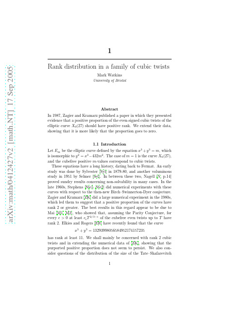
a r X i v :m a t h /0412427v 2 [m a t h .N T ] 17 S e p 200512Mark Watkinsgroups attached to these curves,comment on effects stemming from the arithmetic of m,consider similar questions for quartic twists of X0(32), and discuss random matrix models for these.We briefly review how to compute the central L-value of E m.Thefirst consideration is the sign of the functional equation,which was computed by Birch and Stephens[BS].This is defined byǫ= pǫp where for p=3 we have thatǫp= pne−2πn/√p for p>13and not p≥13as[ZK]claims).Having defined a m(p)for all primes p,we extend it to prime powers via the Hecke relations,and then to all positive integers via multiplicativity.In order to approximate L(E m,1)well,we need to use about C√Rank distribution in a family of cubic twists31.2Numerical data Applying the above method for the cubefree m ≤107with ǫ=+1,we find that about 17.7%of the twists have vanishing central L -value.This is to be compared to 23.3%for the m ≤70000,and 20.5%for m ≤106.If we take the best linear fit to a log-log regression,we find that the number of twists up to x with vanishing central L -value appears to grow like x 0.935.Heuristic models involving the expected size of X as in [ZK]imply that the growth should be more like x 5/6.Stronger models such as those in [CKRS]imply this should be more like Bx 5/6(log x )C for some constants B and C ;in the last section we make remarks about what random matrix theory implies about C .0100000200000300000400000500000600000700000800000012345678910n u m b e r o f e v e n v a n i s h i n g t w i s t s size of twist parameter d in millionsFig.1.1.Number of even vanishing cubic twists of X 0(27)compared to a (dotted)straight line.There is also the question of arithmetic effects of m .Only 6.1%of the prime m in the above range have vanishing central L -value,while 11.3%of the m with two prime factors do,and 17.1%of the m with three prime factors.The number grows to 24.5%for four prime factors,and 35.3%for five prime factors,and is 51.4%for six or more prime factors.However,each of these percentages is about 20%lower than the comparative value when considering only the m ≤106.So even4Mark Watkinsif we restrict to prime m we expect that the proportion of twists withnon-vanishing central L-value tends to zero.Note in this context that3-descent can tell us much about the rank when we limit the number ofprime factors of m(see[C]).For instance,when m is prime and E m haseven functional equation,we know that m≡1,2,5(mod9),and therank is zero in the latter two cases.Thus the6.1%of above might bere-interpreted as18.3%of the cases where descent considerations do notforce the rank to be ing the results of[N],we could similarlyderive such results when m has two prime factors.Also,one can recallthat Elkies(see[E1])has proven that the rank is exactly1for primesm≡4,7(mod9);here in fact the conjecture is that the same is truefor m≡8(mod9).We return to such considerations below when wediscuss random matrix models.We next make some comments about how often various|X|-valuesoccur.Zagier and Kramarz found that26.3%of the even twists form≤70000have rank0and trivial X,while wefind the percentage tobe18.8%for m≤106and14.1%for m≤107.Indeed,already in[ZK]this percentage was noted to be diminishing.More interesting might behow often a given prime divides|X|,under the restriction to rank0twists.For instance,32.4%of the even rank0twists with m≤70000have3dividing|X|.This number increases to40.1%for m≤106,andis45.3%for m≤107.The heuristics of[De]imply a number more like36.1%.There is a strong arithmetic impact from m,as for prime m thepercentage for m≤107is only5.8%.However,this last datum shouldprobably be considered anomalous because of the special role that3plays in the cubic twists.Similarly,2divides|X|about45.7%of the time for even rank0twistswith m≤107,while only42.1%of the time for m≤106and35.5%ofthe time for m≤70000.Here Delaunay predicts58.1%.Here prime mare more likely to cause2-divisibility of|X|,with the percentage herefor m≤107being53.5%.As[ZK]notes,the expectation is that|X|should be of size m1/3≈N1/6for these cubic twists,larger than the expected N1/12in the general case.For5-divisibility of|X|,the per-centage increases from3.6%to5.9%to8.0%.It seems unlikely thatthese percentages(for p=3)will climb all the way to100%,and with-out a better guess,one could posit that they are tending toward thenumber suggested by the Delaunay heuristic.In Table1.1,the“r>0”column counts percentages of curves for which the central L-value van-ishes,while the other four columns denote how often a given primedivides the|X|-value of a nonvanishing twist.Rank distribution in a family of cubic twists5 Table1.1.Data for cubic twistsm≤10522.937.333.7 3.9 1.2m≤10620.542.140.1 5.9 2.4m≤10717.745.745.38.0 3.7prime m≤107 6.153.5 5.814.58.2 Delaunay58.336.120.714.56Mark Watkinsin the question of extra vanishing,and seemed sufficient to answer the question posed by[ZK]on whether the rate remained constant.With today’s technology,extending the experiment to m≤108should be feasible,as should a similar experiment looking at cubic twists with odd functional equation.As stated in[ZK],the computation of the a m(n)takes time O(log n)if n is prime and O(1)time otherwise(using the multiplicativity relations, viewing the values for the primes dividing n as taking negligible time as they are already computed).We computed the values of a1(p)for p≤109once-and-for-all ahead of time,and then read these from disk as needed.Additionally,tricks such as fast modular exponentiation were used to speed up the computation of m(p−1)/3mod p.Similarly,the√computing of e−2πn/N and then for each n multiplied these together as needed to get the desired value.For the computation of L(E m,1),and the question of how far the infinite sum need be computed,we followed a method similar to that of[ZK],calculating the|X|-value S m=T2x should approximate(for small x)the probability density function for values of L(E d,1),where N∼log X and we integrate X0P E(N,x)dx to get an expected proba-Rank distribution in a family of cubic twists7 bility that L(E d,1)is less than X.The idea is that we know that the actual values of L(E d,1)are discretised(due to the Birch–Swinnerton-Dyer formula),and thus we declare(in a somewhat arbitrary manner) sufficiently small values of L(E d,1)to indicate that in fact we have L(E d,1)=0.We recall that BSD implies we haveL(E d,1)|T d|2whereΩd is the real period of E d,the c p are Tamagawa numbers,X d is the Shafarevitch–Tate group,and T d is the torsion group of E d.We are thus thinking of|X d|(which is a square)as our discretised vari-able,with everything else being computable.When d>2the torsiongroup is trivial.For cubefree d we have thatΩd=Ω1/d1/3,except when 9|d in which case we haveΩd=3Ω1/d1/3.Note that in definition(8) of[CKRS],quadratic twists that are not relatively prime to the conduc-tor are excluded;we will similarly exclude twists that are divisible by3, though one could deal with them via making appropriate corrections. For the Tamagawa product we have that c3=3when d≡±1(mod9), c3=2when d≡±2(mod9),and c3=1otherwise,while c p=3for primes p≡1(mod3)and c p=1for primes p≡2(mod3).Given this divergent behaviour based upon prime divisibility,as in Conjecture1 of[CKRS]we decided to restrict to prime twists,and additionally split the primes into congruence classes modulo9.Indeed,it is calculable that the sign of the functional equation is odd when our prime twist d is congruent to4,7,8(mod9),and by3-descent we can verify that the rank is zero when d is2or5(mod9).Moreover,again by3-descent,we know that the rank is at most2(and the functional equation is even) when d puting as with equation(23)in[CKRS]we get the following:Question1.4.1Let V T be the set of primes d less than T congruent to 1modulo9with L(E d,1)=0.Is there some constant c=0such thatd∈V T1∼cT5/6(log T)−5/8?Assuming an affirmative answer,our data give a constant of approxi-mately c=1/6.The argument is similar for quartic twists of X0(32)or sextic twists of X0(27),and we can expect asymptotics for prime twists of order T7/8(log T)−5/8and T11/12(log T)−5/8,and upon restricting to various congruence classes we should get appropriate constants in front8Mark Watkinsof these.Via techniques from prime number theory and considerations from Tamagawa numbers,one should be able to argue as in[CKRS]to get an asymptotic for all cubefree twists.Finally we derive a version of Conjecture2of[CKRS]suitable for cubic,quartic,and sextic twists.For cubic twists,for a given prime p≡1(mod3)there are3solutions to a2+3b2=4p with a≡2(mod3), which correspond to the three possibilities for the Frobenius trace a p. The argument given from(27)-(31)in[CKRS]does not differ(see below), and so we get the following:Question1.4.2Let p≥5be prime,and for1≤q≤p−1let F q p(T)be the set of cubefree positive integers d≡q(mod p)that are less than T such that x3+y3=d has even functional equation.Letting a d(p)be the p th trace of Frobenius for x3+y3=d(where d need not be cubefree),do we havelimT→∞ d∈F Y p(T)1 d∈F Zp(T)1 = p+1−a Z(p)?We can also make a similar calculation for quartic and sextic twists. In Tables1.2-1.4below we list vanishing probabilities in support of an affirmative answer to the above question;the c-column represents which congruence class is used.For p=7the ratios should be[√9:√9:√21].We also have some data(see Tables1.6-1.8)for the vanishing fre-quencies for positive quartic twists of X0(32).For p=5the ratios should be given by √4:√10 ;for p=13they should be √10:√20 .The heuristic for Conjecture2in[CKRS]is based upon supposed cancellation from a quadratic character,whereas in our cubic twist case the source of cancellation is perhaps not so transparent.Therefore we go through the details.We have thatd∈F q p(T)L(E d,1/2)k= d∈F q p(T) ∞ n=1a d(n)n,where b m(n)= n=n1···n k a m(n1)···a m(n k)with the sum being over all ways of writing n as a product of k positive factors.If we invert the order of summation in this last expression,the sum over d should typically have much cancellation since the b d(n)are essentially randomly distributed.This,however,is not the case for n that are a power of p,Rank distribution in a family of cubic twists9 as here the value of a d(p r)isfixed since d isfixed modulo p.Thus we should get a main contribution in the above by restricting to values of n that are powers of p(indeed,if we did this argument with no congruence restriction we would expect n=1to give the main term).As in(31)of [CKRS]we thus get thatd∈F q p(T)L(E d,1/2)k∼ d∈F q p(T) p r b d(p r)p r k== p10Mark Watkins[De] C.Delaunay,Heuristics on Tate-Shafarevitch Groups of Elliptic Curves Defined over Q.Experiment.Math.10(2001),no.2,191–196.[E1]N.D.Elkies,Heegner point computations.In Algorithmic Number Theory, Proceedings of the First International Symposium(ANTS-I)held at Cornell University,Ithaca,New York,May6–9,1994.Edited by L.M.Adleman and M.-D.Huang.Lecture Notes in Computer Science,877.Springer-Verlag, Berlin(1994),122–133.[E2]N. D.Elkies,Curves Dy2=x3−x of odd analytic rank.In Algo-rithmic number theory,Proceedings of the5th International Symposium (ANTS-V)held at the University of Sydney,Sydney,July7–12,2002.Edited by C.Fieker and D.R.Kohel.Lecture Notes in Computer Sci-ence,2369.Springer-Verlag,Berlin(2002),244–251.Available online at /math.NT/0208056[ER]N.D.Elkies,N.F.Rogers,Elliptic curves x3+y3=k of high rank.In Algorithmic number theory,Proceedings of the6th International Sym-posium(ANTS-VI)held at the University of Vermont,Burlington,VT, June13–18,2004.Edited by D.Buell.Lecture Notes in Computer Sci-ence,3076.Springer-Verlag,Berlin(2004),184–193.Available online at /math.NT/0403116[L] D.B.Lieman,Nonvanishing of L-series associated to cubic twists of elliptic curves.Ann.of Math.(2)140(1994),no.1,81–108.[M1]L.Mai,The analytic rank of a family of elliptic curves.Canad.J.Math.45(1993),no.4,847–862.[M2]L.Mai,The average analytic rank of a family of elliptic curves.J.Number Theory45(1993),no.1,45–60.[N]T.Nagell,L’analyse ind´e termin´e e de degr´e sup´e rieur.M´e morial des Sci-ences Math´e matiques,Fascicule XXXIX,Paris,1929.[RVZ] F.Rodriguez Villegas,D.Zagier,Which primes are sums of two cubes?In Number theory,Proceedings of the Fourth Conference of the Canadian Number Theory Association held at Dalhousie University,Halifax,Nova Scotia,July2–8,1994.Edited by K.Dilcher.CMS Conference Proceedings,15.Published by the American Mathematical Society,Providence,RI;forthe Canadian Mathematical Society,Ottawa,ON,(1995),295–306. [Sel] E.S.Selmer,The Diophantine equation ax3+by3+cz3=0.Acta Math.85(1951),203–362,Acta Math.92(1954),191–197.[Ste1]N.M.Stephens,Conjectures concerning elliptic curves.Bull.Amer.Math.Soc.73(1967),160–163.[Ste2]N.M.Stephens,The diophantine equation X3+Y3=DZ3and the conjectures of Birch and Swinnerton-Dyer.J.Reine Angew.Math.231 (1968),121–162.[ST] C.L.Stewart,J.Top,On Ranks of Twists of Elliptic Curves and Power-Free Values of Binary Forms.J.Amer.Math.Soc.,8(1995),no.4,943–973. [Syl]J.J.Sylvester,On Certain Ternary Cubic-Form Equations.American Journal of Mathematics,2(1879),no.3,280–285,no.4,357–393,3(1880), no.1,58–88,no.2,179–189.[ZK] D.Zagier,G.Kramarz,Numerical Investigations Related to the L-series of Certain Elliptic Curves.J.Indian Math.Soc.52(1987),51–69.Rank distribution in a family of cubic twists11Table1.2.p=5,X0(27) 11404638386120.167 21405498385700.168 31406138385750.168 41407508386370.168c#r>0#curvesTable1.4.p=11,X0(27) 1649893784100.172 2652113784080.172 3650013784300.172 4650083784440.172 5649563784230.172 6652083784260.172 7650543784110.172 8647733784220.171 9651643783960.172 10653383784010.173c#r>0#curvesTable1.6.p=5,X0(32) 11560977490890.208 21041367491070.139 32368617491250.316 42159447491820.288c#r>0#curvesTable1.8.p=11,X0(32) 1826533410920.242 2827823410700.243 3825813410690.242 4823923410720.242 5828063411130.243 6824483410610.242 7826613411080.242 8823883410450.242 9827203410910.243 10829483410830.243c#r>0#curves。
2024年高三英语统计学分析单选题30题1.The average height of a group of people is calculated by adding up all the heights and then dividing by the _____.A.number of peopleB.sum of heightsC.difference in heightsD.product of heights答案:A。
本题考查平均数的计算方法。
平均数是所有数据之和除以数据的个数,这里就是把所有人的身高加起来然后除以人数。
选项B“sum of heights”是身高总和,不是计算平均数的除数。
选项C“difference in heights”是身高差,与平均数计算无关。
选项D“product of heights”是身高乘积,也与平均数计算无关。
2.In a statistical survey, the mode is the value that _____.A.appears most frequentlyB.has the highest sumC.is the averageD.is the middle value答案:A。
本题考查众数的概念。
众数是一组数据中出现次数最多的数值。
选项B“has the highest sum”是和最大,与众数无关。
选项C“is the average”是平均数,与众数不同。
选项D“is the middle value”是中位数,不是众数。
3.The median of a set of data is found by arranging the data in orderand then finding the _____.rgest valueB.smallest valueC.middle valueD.average value答案:C。
《概率论与数理统计》基本名词中英文对照表英文中文Probability theory 概率论mathematical statistics 数理统计deterministic phenomenon 确定性现象random phenomenon 随机现象sample space 样本空间random occurrence 随机事件fundamental event 基本事件certain event 必然事件impossible event 不可能事件random test 随机试验incompatible events 互不相容事件frequency 频率classical probabilistic model 古典概型geometric probability 几何概率conditional probability 条件概率multiplication theorem 乘法定理Bayes’s formula 贝叶斯公式Prior probability 先验概率Posterior probability 后验概率Independent events 相互独立事件Bernoulli trials 贝努利试验random variable 随机变量probability distribution 概率分布distribution function 分布函数discrete random variable 离散随机变量distribution law 分布律hypergeometric distribution 超几何分布random sampling model 随机抽样模型binomial distribution 二项分布Poisson distribution 泊松分布geometric distribution 几何分布probability density 概率密度continuous random variable 连续随机变量uniformly distribution 均匀分布exponential distribution 指数分布numerical character 数字特征mathematical expectation 数学期望variance 方差moment 矩central moment 中心矩n—dimensional random variable n—维随机变量two-dimensional random variable 二维离散随机变量joint probability distribution 联合概率分布joint distribution law 联合分布律joint distribution function 联合分布函数boundary distribution law 边缘分布律boundary distribution function 边缘分布函数exponential distribution 二维指数分布continuous random variable 二维连续随机变量joint probability density 联合概率密度boundary probability density 边缘概率密度conditional distribution 条件分布conditional distribution law 条件分布律conditional probability density 条件概率密度covariance 协方差dependency coefficient 相关系数normal distribution 正态分布limit theorem 极限定理standard normal distribution 标准正态分布logarithmic normal distribution 对数正态分布covariance matrix 协方差矩阵central limit theorem 中心极限定理Chebyshev’s inequality 切比雪夫不等式B ernoulli’s law of large numbers 贝努利大数定律statistics 统计量simple random sample 简单随机样本sample distribution function 样本分布函数sample mean 样本均值sample variance 样本方差sample standard deviation 样本标准差sample covariance 样本协方差sample correlation coefficient 样本相关系数order statistics 顺序统计量sample median 样本中位数sample fractiles 样本极差sampling distribution 抽样分布parameter estimation 参数估计estimator 估计量estimate value 估计值unbiased estimator 无偏估计unbiassedness 无偏性biased error 偏差mean square error 均方误差relative efficient 相对有效性minimum variance 最小方差asymptotic unbiased estimator 渐近无偏估计量uniformly estimator 一致性估计量moment method of estimation 矩法估计maximum likelihood method of estimation 极大似然估计法likelihood function 似然函数maximum likelihood estimator 极大似然估计值interval estimation 区间估计hypothesis testing 假设检验statistical hypothesis 统计假设simple hypothesis 简单假设composite hypothesis 复合假设rejection region 拒绝域acceptance domain 接受域test statistics 检验统计量linear regression analysis 线性回归分析。
•字餌蓀索多元柯西分布及其特性李子言(华中师范大学数学与统计学学院湖北•武汉430079)摘要柯西分布是一种基于中位数与中位数绝对偏差的分布,在数学、物理学等中都有重要的意义和作用。
其 中,一元柯西分布被大众所熟知,本文以此引入多元柯西分布的分析,初步介绍了多元柯西分布的定义和相关性质。
关键词多元柯西分布特征函数密度函数中图分类号:〇212文献标识码:ADOI : 10.16400/j .cnki .kjdk .2021.10.020Multivariate Cau c h y Distribution and i t s CharacteristicsLI Ziyan(School o f Mathematics and Statistics, Central China Normal University, Wuhan, Hubei 430079)Abstract Cauchy distribution is a kind of distribution based on median and absolute deviation of median , which hasimportant significance and role in mathematics , physics and so on . Among them , the univariate Cauchy distribution is well known by the public . This paper introduces the analysis of multivariate Cauchy distribution , and introduces the definition and related properties of multivariate Cauchy distribution .Keywords multivariate Cauchy distribution ; characteristic function ; density function 柯西分布也叫作柯西-洛伦兹分布,它是以奧古斯丁 • 路易•柯西与亨德里克•洛伦兹名字命名的连续概率分 布,目前最广泛应用的是一元柯西分布,它的概率密度函 数为:/(x ;x 〇-r ) = ^[(^7T 7]其中心为分布峰值位置的位置参数,y 为最大值一半处 的一半宽度的尺度参数。