Using Soft CSPs for Approximating Pareto-Optimal Solution Sets
- 格式:pdf
- 大小:132.37 KB
- 文档页数:8

一种基于 Pareto 云隶属度的 MOPSO 算法高志强;刘丽霞;刘悦;邱晓华;于广浩【期刊名称】《中国科技论文》【年(卷),期】2015(000)014【摘要】An improved MOPSO algorithm based on Pareto cloud membership is proposed to cope the problem of Pareto-Sort,as well as convergence and variety of MOPSO.First,Logistic map is adopted to initialize the population combined with cuckoo search to enhance the ability on global searching.Meanwhile,cloud membership is used to measure global best and personal best solution in order to maintain the external archive.Finally,experiment results on ZDT test function set show that the proposed al-gorithm outperforms on both convergence and variety than MOPSO and NSGA-Ⅱ.%为定量解决非支配解排序问题,并兼顾多目标粒子群优化算法(multi-objective particle swarm optimization,MOPSO)的收敛性和多样性,提出了一种基于 Pareto 云隶属度的 MOPSO 算法。
利用Logistic 混沌映射优化种群的初始空间分布并融合布谷鸟搜索(cuckoo search,CS)指导粒子跳出局部陷阱,以增强算法的全局寻优能力。

多目标多约束优化问题算法多目标多约束优化问题是一类复杂的问题,需要使用特殊设计的算法来解决。
以下是一些常用于解决这类问题的算法:1. 多目标遗传算法(Multi-Objective Genetic Algorithm, MOGA):-原理:使用遗传算法的思想,通过进化的方式寻找最优解。
针对多目标问题,采用Pareto 前沿的概念来评价解的优劣。
-特点:能够同时优化多个目标函数,通过维护一组非支配解来表示可能的最优解。
2. 多目标粒子群优化算法(Multi-Objective Particle Swarm Optimization, MOPSO):-原理:基于群体智能的思想,通过模拟鸟群或鱼群的行为,粒子在解空间中搜索最优解。
-特点:能够在解空间中较好地探索多个目标函数的Pareto 前沿。
3. 多目标差分进化算法(Multi-Objective Differential Evolution, MODE):-原理:差分进化算法的变种,通过引入差分向量来生成新的解,并利用Pareto 前沿来指导搜索过程。
-特点:对于高维、非线性、非凸优化问题有较好的性能。
4. 多目标蚁群算法(Multi-Objective Ant Colony Optimization, MOACO):-原理:基于蚁群算法,模拟蚂蚁在搜索食物时的行为,通过信息素的传递来实现全局搜索和局部搜索。
-特点:在处理多目标问题时,采用Pareto 前沿来评估解的质量。
5. 多目标模拟退火算法(Multi-Objective Simulated Annealing, MOSA):-原理:模拟退火算法的变种,通过模拟金属退火的过程,在解空间中逐渐减小温度来搜索最优解。
-特点:能够在搜索过程中以一定的概率接受比当前解更差的解,避免陷入局部最优解。
这些算法在解决多目标多约束优化问题时具有一定的优势,但选择合适的算法还取决于具体问题的性质和约束条件。


软件简介1、LINDO主要求解线性规划、整数规划、二次规划问题。
现在版本好像是6.1。
2、GINO最初这也是一个求非线性规划的工具,甚至她还用来求解一些非线性的方程根。
它的特点是:包含了丰富的数学函数,尤其是概率函数!但是随着像Mathematica/Matlab的迅速发展,他逐渐的消亡,并演化为现在的函数引擎LINDO API,现在版本2.0。
3、LINGO/LINGO NLLINGO8.0有两部分:LINGO and LINGO NL,他们分别用于求解线性、整数规划以及非线性、线性、整数规划问题,现在就统一成为了LINGO,它与LINDO的主要主要区别在于:她内建了建模语言,可以简约的得描述大规模的优化问题。
现在版本是9.0。
4、What's the best这是一个组件,主要处理由Excell/Access 生成数据文件的规划问题,安装之后会在你的Office中添加一个名为What's the best的宏,启用后会在Excell中生成一个工具条,就像Adobe的pdf插件一样。
现在版本是7.0。
LINDO是一种专门用于求解数学规划问题的软件包。
由于LINDO执行速度很快、易于方便输入、求解和分析数学规划问题。
因此在数学、科研和工业界得到广泛应用。
LINDO主要用于解线性规划、非线性规划、二次规划和整数规划等问题。
也可以用于一些非线性和线性方程组的求解以及代数方程求根等。
LINDO中包含了一种建模语言和许多常用的数学函数(包括大量概论函数),可供使用者建立规划问题时调用。
一般用LINDO(Linear Interactive and Discrete Optimizer)解决线性规划(LP—Linear Programming)。
整数规划(IP—Integer Programming)问题。
其中LINDO 6 .1 学生版至多可求解多达300个变量和150个约束的规划问题。

parote前沿解集
一、多目标优化问题的目标往往量纲不同、互相冲突,难以像单目标优化问题一样直接比较目标值来确定最优解。
二、Pareto占优思想是一种评价多目标问题解优劣的处理方法,Pareto最优解集是指可行域中所有非劣解的集合(就是你所说的约束变量(x1、x2、……xn)的集合),Pareto最优前沿是Pareto最优解集对应目标值的集合(就是你所说的目标函数空间的值(f1 f2... fn)的集合)。
三、优化问题就是需要人们采用某种方法\技术,将问题的目标进行优化,即评价指标都是针对目标空间上的值来进行的,其对应的解决方法就是问题的解。
评价算法的求解质量优劣,就是你能不能求得目标值更优的解。
四、世代距离(GD)是评价多目标算法在求解质量方面优劣的一种方法,所列举论文中的表述正确,难点在于多目标优化问题中难以确定Pareto最优前沿,在计算GD指标时一般以现有算法的最优解集对应的目标值组合成近似Pareto最优前沿代替真实Pareto最优前沿。
收稿日期:20210909;修回日期:20211028 基金项目:贵州省科技计划项目重大专项项目(黔科合重大专项字[2018]3002,黔科合重大专项字[2016]3022);贵州省公共大数据重点实验室开放课题(2017BDKFJJ004);贵州省教育厅青年科技人才成长项目(黔科合KY字[2016]124) 作者简介:兰周新(1998),男,硕士研究生,主要研究方向为机器学习(lzxc511@163.com);何庆(1982),男(通信作者),副教授,博士,主要研究方向为智能算法、大数据应用.
多策略融合算术优化算法及其工程优化兰周新a,b,何 庆a,b(贵州大学a.大数据与信息工程学院;b.贵州省公共大数据重点实验室,贵阳550025)
摘 要:针对算术优化算法(AOA)在搜索过程中容易陷入局部极值点、收敛速度慢以及求解精度低等缺陷,提出一种多策略集成的算术优化算法(MFAOA)。首先,采用Sobol序列初始化AOA种群,增加初始个体的多样性,为算法全局寻优奠定基础;然后,重构数学优化器加速函数(MOA),权衡全局搜索与局部开发过程的比重;最后,利用混沌精英突变策略,改善算法过于依赖当前最优解的问题,增强算法跳出局部极值的能力。选用12个基准函数和部分CEC2014测试函数进行实验仿真,结果表明MFAOA在求解精度和收敛速度上均有明显的提升;另外,通过对两个工程实例进行优化,验证了MFAOA在工程优化问题上的可行性。关键词:算术优化算法;Sobol序列;数学优化器加速函数;混沌精英突变;工程优化中图分类号:TP18 文献标志码:A 文章编号:10013695(2022)03019075806doi:10.19734/j.issn.10013695.2021.09.0358
Multistrategyfusionarithmeticoptimizationalgorithmanditsapplicationofprojectoptimization
Simulating Soft Shadowswith Graphics HardwarePaul S.Heckbert and Michael HerfJanuary15,1997CMU-CS-97-104School of Computer ScienceCarnegie Mellon UniversityPittsburgh,PA15213email:ph@,herf+@World Wide Web:/phThis paper was written in April1996.An abbreviated version appeared in[Michael Herf and Paul S.Heckbert,Fast Soft Shadows,Visual Proceedings,SIGGRAPH96,Aug.1996,p.145].AbstractThis paper describes an algorithm for simulating soft shadows at interactive rates using graphics hardware.On current graphics workstations,the technique can calculate the soft shadows cast by moving,complex objects onto multiple planar surfaces in about a second.In a static,diffuse scene,these high quality shadows can then be displayed at30Hz,independent of the number and size of the light sources.For a diffuse scene,the method precomputes a radiance texture that captures the shadows and other brightness variations on each polygon.The texture for each polygon is computed by creating registered projections of the scene onto the polygon from multiple sample points on each light source,and averaging the resulting hard shadow images to compute a soft shadow image. After this precomputation,soft shadows in a static scene can be displayed in real-time with simple texture mapping of the radiance textures.All pixel operations employed by the algorithm are supported in hardware by existing graphics workstations. The technique can be generalized for the simulation of shadows on specular surfaces.This work was supported by NSF Young Investigator award CCR-9357763.The views and conclusions contained in this document are those of the authors and should not be interpreted as representing the official policies,either expressed or implied,of NSF or the ernment.Keywords:penumbra,texture mapping,graphics workstation, interaction,real-time,SGI Reality Engine.1IntroductionShadows are both an important visual cue for the perception of spatial relationships and an essential component of realistic images. Shadows differ according to the type of light source causing them: point light sources yield hard shadows,while linear and area(also known as extended)light sources generally yield soft shadows with an umbra(fully shadowed region)and penumbra(partially shad-owed region).The real world contains mostly soft shadows due to thefinite size of sky light,the sun,and light bulbs,yet most computer graphics rendering software simulates only hard shadows,if it simulates shadows at all.Excessive sharpness of shadow edges is often a telltale sign that a picture is computer generated.Shadows are even less commonly simulated with hardware ren-dering.Current graphics workstations,such as Silicon Graphics (SGI)and Hewlett Packard(HP)machines,provide z-buffer hard-ware that supports real-time rendering of fairly complex scenes. Such machines are wonderful tools for computer aided design and visualization.Shadows are seldom simulated on such machines, however,because existing algorithms are not general enough,or they require too much time or memory.The shadow algorithms most suitable for interaction on graphics workstations have a cost per frame proportional to the number of point light sources.While such algorithms are practical for one or two light sources,they are impractical for a large number of sources or the approximation of extended sources.We present here a new algorithm that computes the soft shad-ows due to extended light sources.The algorithm exploits graphics hardware for fast projective(perspective)transformation,clipping, scan conversion,texture mapping,visibility testing,and image av-eraging.The hardware is used both to compute the shading on the surfaces and to display it,using texture mapping.For diffuse scenes,the shading is computed in a preprocessing step whose cost is proportional to the number of light source samples,but while the scene is static,it can be redisplayed in time independent of the num-ber of light sources.The method is also useful for simulating the hard shadows due to a large number of point sources.The memory requirements of the algorithm are also independent of the number of light source samples.1.1The IdeaFor diffuse scenes,our method works by precomputing,for each polygon in the scene,a radiance texture[12,14]that records the color(outgoing radiance)at each point in the polygon.In a diffuse scene,the radiance at each surface point is view independent,so it can be precomputed and re-used until the scene geometry changes. This radiance texture is analogous to the mesh of radiosity values computed in a radiosity algorithm.Unlike a radiosity algorithm, however,our algorithm can compute this texture almost entirely in hardware.The key idea is to use graphics hardware to determine visibility and calculate shading,that is,to determine which portions of a surface are occluded with respect to a given extended light source, and how brightly they are lit.In order to simulate extended light sources,we approximate them with a number of light sample points, and we do visibility tests between a given surface point and each light sample.To keep as many operations in hardware as possible, however,we do not use a hemicube[7]to determine visibility. Instead,to compute the shadows for a single polygon,we render the scene into a scratch buffer,with all polygons except the one being shaded appropriately blackened,using a special projective projection from the point of view of each light sample.These views are registered so that corresponding pixels map to identical points on the polygon.When the resulting hard shadow images are averaged, a soft shadow image results(figure1).This image is then used directly as a texture on the polygon in order to simulate shadows correctly.The textures so computed are used for real-time display until the scene geometry changes.In the remainder of the paper,we summarize previous shadow algorithms,we present our method for diffuse scenes in more detail, we discuss generalizations to scenes with specular and general re-flectance,we present our implementation and results,and we offer some concluding remarks.2Previous Work2.1Shadow AlgorithmsWoo et al.surveyed a number of shadow algorithms[19].Here we summarize soft shadows methods and methods that run at inter-active rates.Shadow algorithms can be divided into three categories: those that compute everything on thefly,those that precompute just visibility,and those that precompute shading.Computation on the Fly.Simple ray tracing computes everything on thefly.Shadows are computed on a point-by-point basis by tracing rays between the surface point and a point on each light source to check for occluders.Soft shadows can be simulated by tracing rays to a number of points distributed across the light source [8].The shadow volume approach is another method for computing shadows on thefly.With this method,one constructs imaginary surfaces that bound the shadowed volume of space with respect to each point light source.Determining if a point is in shadow then reduces to point-in-volume testing.Brotman and Badler used an extended z-buffer algorithm with linked lists at each pixel to support soft shadows using this approach[4].The shadow volume method has also been used in two hardware implementations.Fuchs et ed the pixel processors of the Pixel Planes machine to simulate hard shadows in real-time[10]. Heidmann used the stencil buffer in advanced SGI machines[13]. With Heidmann’s algorithm,the scene must be rendered through the stencil created from each light source,so the cost per frame is proportional to the number of light sources times the number of polygons.On1991hardware,soft shadows in a fairly simple scene required several seconds with his algorithm.His method appears to be one of the algorithms best suited to interactive use on widely available graphics hardware.We would prefer,however,an algorithm whose cost is sublinear in the number of light sources.A simple,brute force approach,good for casting shadows of objects onto a plane,is tofind the projective transformation that projects objects from a point light onto a plane,and to use it to draw each squashed,blackened object on top of the plane[3],[15, p.401].This algorithm effectively multiplies the number of objects in the scene by the number of light sources times the number of receiver polygons onto which shadows are being cast,however, so it is typically practical only for very small numbers of light sources and receivers.Another problem with this method is that occluders behind the receiver will cast erroneous shadows,unless extra clipping is done.Precomputation of Visibility.Instead of computing visibility on thefly,one can precompute visibility from the point of view of each light source.The z-buffer shadow algorithm uses two(or more)passes of z-buffer rendering,first from the light sources,and then from the eye[18].The z-buffers from the light views are used in thefinalFigure 1:Hard shadow images from 22grid of sample points on lightsource.Figure 2:Left:scene with square light source (foreground),triangular occluder (center),and rectangular receiver (background),with shadows on receiver.Center:Approximate soft shadows resulting from 22grid of sample points;the average of the four hard shadow images in Figure 1.Right:Correct soft shadow image (generated with 1616sampling).This image is used as the texture on the receiver at left.pass to determine if a given 3-D point is illuminated with respect to each light source.The transformation of points from one coordinate system to another can be accelerated using texture mapping hard-ware [17].This latter method,by Segal et al.,achieves real-time rates,and is the other leading method for interactive shadows.Soft shadows can be generated on a graphics workstation by rendering the scene multiple times,using different points on the extended light source,averaging the resulting images using accumulation buffer hardware [11].A variation of the shadow volume approach is to intersect these volumes with surfaces in the scene to precompute the umbra and penumbra regions on each surface [16].During the final rendering pass,illumination integrals are evaluated at a sparse sampling of pixels.Precomputation of Shading.Precomputation can be taken fur-ther,computing not just visibility but also shading.This is most relevant to diffuse scenes,since their shading is view-independent.Some of these methods compute visibility continuously,while oth-ers compute it discretely.Several researchers have explored continuous visibility methods for soft shadow computation and radiosity mesh generation.With this approach,surfaces are subdivided into fully lit,penumbra,and umbra regions by splitting along lines or curves where visibility changes.In Chin and Feiner’s soft shadow method,polygons are split using BSP trees,and these sub-polygons are then pre-shaded [6].They achieved rendering times of under a minute for simple scenes.Drettakis and Fiume used more sophisticated computational geometry techniques to precompute their subdivision,and reported rendering times of several seconds [9].Most radiosity methods discretize each surface into a mesh of elements and then use discrete methods such as ray tracing or hemicubes to compute visibility.The hemicube method computes visibility from a light source point to an entire hemisphere by pro-jecting the scene onto a half-cube [7].Much of this computation can be done in hardware.Radiosity meshes typically do not resolve shadows well,however.Typical artifacts are Mach bands along the mesh element boundaries and excessively blurry shadows.Most radiosity methods are not fast enough to support interactive changes to the geometry,however.Chen’s incremental radiosity method is an exception [5].Our own method can be categorized next to hemicube radiosity methods,since it also precomputes visibility discretely.Its tech-nique for computing visibility also has parallels to the method of flattening objects to a plane.2.2Graphics HardwareCurrent graphics hardware,such as the Silicon Graphics Reality Engine [1],can projective-transform,clip,shade,scan convert,and texture tens of thousands of polygons in real-time (in 1/30sec.).We would like to exploit the speed of this hardware to simulate soft shadows.Typically,such hardware supports arbitrary 44homogeneous transformations of planar polygons,clipping to any truncated pyra-midal frustum (right or oblique),and scan conversion with z-buffering or overwriting.On SGI machines,Phong shading (once per pixel)is not possible,but faceted shading (once per polygon)and Gouraud shading (once per vertex)are supported.Phong shadingcan be simulated by splitting polygons into small pieces on input.A common,general form for hardware-supported illumination is dif-fuse reflection from multiple point spotlight sources,with a texture mapped reflectance function and attenuation:cos cos2where,as shown in Figure3,is a3-D point on a reflective surface,and isa point on a light source,is polar angle(angle from normal)at,is the angle at,is the distance between and,,,and are functions of and,is outgoing radiance at point for color channel,due to either emission or reflection,a is ambient radiance,is reflectance,is a Boolean visibility function that equals1if point is visible from point,else0,cos+max cos0,for backface testing,andthe integral is over all points on all light sources,with respect to,which is an infinitesimal area on a light source.The inputs to the problem are the geometry,the reflectance, and emitted radiance on all light sources,the ambient radi-ance a,and the output is the reflected radiance function.Figure3:Geometry for direct illumination.The radiance at point on the receiver is being calculated by summing the contributions from a set of point light sources at on light.3.1Approximating Extended Light SourcesAlthough such integrals can be solved in closed form for planar surfaces with no occlusion(1),the complexity of the visibility function makes these integrals intractable in the general case.We can compute approximations to the integral,however,by replacing each extended light source by a set of point light sources:1where is a3-D Dirac delta function,is sample point on light source,and is the area associated with this sample point. Typically,each sample on a light source has equal area:, where is the area of light source.With this approximation,the radiance of a reflective surface point can be computed by summing the contributions over all sample points on all light sources:a1cos+cos+2(2)Each term in the inner summation can be regarded as a hard shadow image resulting from a point light source at,where is a function of screen.That summand consists of the product of three factors.Thefirst one,which is an area times the reflectance of the receiving polygon, can be calculated in software.The second factor is the cosine of the angle on the receiver,times the cosine of the angle on the lightb+e x Figure4:Pyramid with parallelogram base.Faces of pyramid are marked with their plane equations.source,times the radiance of the light source,divided by2.This can be computed in hardware by rendering the receiver polygon with a single spotlight at turned on,using a spotlight exponent of1and quadratic attenuation.On machines that do not support Phong shading,we will have tofinely subdivide the polygon.The third factor is visibility between a point on a light source and each point on the receiver.Visibility can be computed by projecting all polygons between light source point and the receiver onto the receiver.We want to simulate soft shadows as quickly as possible.To take full advantage of the hardware,we can precompute the shading for each polygon using the formula above,and then display views of the scene from moving viewpoints using real-time texture mapping and z-buffering.To compute soft shadow textures,we need to generate a number of hard shadow images and then average them.If these hard shadow images are not registered(they would not be,using hemi-cubes), then it would be necessary to resample them so that corresponding pixels in each hard shadow image map to the same surface point in 3-D.This would be very slow.A faster alternative is to choose the transformation for each projection so that the hard shadow images are perfectly registered with each other.For planar receiver surfaces,this is easily accomplished by ex-ploiting the capabilities of projective transformations.If wefit a parallelogram around the receiver surface of interest,and then con-struct a pyramid with this as its base and the light point as its apex, there is a44homogeneous transformation that will map such a pyramid into an axis-aligned box,as described shortly.The hard shadow image due to sample point on light is created by loading this special transformation matrix and rendering the receiver polygon.The polygon is illuminated by the ambient light plus a single point light source at,using Phong shading or a good approximation to it.The visibility function is then computed by rendering the remainder of the scene with all surfaces shaded as if they were the receiver illuminated by ambient light:r ar g ag b ab.This is most quickly done with z-buffering off,and clipping to a pyramid with the receiver polygon as its base. Drawing each polygon with an unsorted painter’s algorithm suffices here because all polygons are the same color,and after clipping, the only polygon fragments remaining will lie between the light source and the receiver,so they all cast shadows on the receiver. To compute the weighted average of the hard shadow images so created,we use the accumulation buffer.3.3Projective Transformation of a Pyramid to a BoxWe want a projective(perspective)transformation that maps a pyramid with parallelogram base into a rectangular parallelepiped. The pyramid lies in object space,with coordinates o o o.It has apex and its parallelogram base has one vertex at and edge vectors x and y(bold lower case denotes a3-D point or vector). The parallelepiped lies in what we will call unit screen space,with coordinates u u u.Viewed from the apex,the left and right sides of the pyramid map to the parallel planes u0and u1, the bottom and top map to u0and u1,and the base plane anda plane parallel to it through the apex map to u1and u, respectively.Seefigure4.A44homogeneous matrix effecting this transformation can be derived from these conditions.It will have the form:0001020310111213000130313233and the homogeneous transformation and homogeneous division to transform object space to unit screen space are:1ooo1anduuu1The third row of matrix takes this simple form because a constant uvalue is desired on the base plane.The homogeneous screen coordinates,,and are each affine functions of o,o,and o (that is,linear plus translation).The constraints above specify the value of each of the three coordinates at four points in space–just enough to uniquely determine the twelve unknowns in.The coordinate,for example,has value1at the points, x,and y,and value0at.Therefore,the vector w y xis normal to any plane of constant,thusfixing thefirst three elements of the last row of the matrix within a scale factor: 303132w w.Setting to0at and1at constrains33w w and w1w w,where w.Thefirst two rows of can be derived similarly(seefigure4).The result is:x xx x xy x xz x xy yx y yy y yz y y0001w wx w wy w wz w wwherex w yy x ww y xandx1x xy1y yw1w w Blinn[3]uses a related projective transformation for the genera-tion of shadows on a plane,but his is a projection(it collapses3-D to2-D),while ours is3-D to3-D.We use the third dimension for clipping.3.4Using the TransformationTo use this transformation in our shadow algorithm,wefirstfit a parallelogram around the receiver polygon.If the receiver is a rectangle or other parallelogram,thefit is exact;if the receiver is a triangle,then wefit the triangle into the lower left triangle of the parallelogram;and for more general polygons with four or more sides,a simple2-D bounding box in the plane of the polygon can be used.It is possible to go further with projective transformations, mapping arbitrary planar quadrilaterals into squares(using the ho-mogeneous texture transformation matrix of OpenGL,for example). We assume for simplicity,however,that the transformation between texture space(the screen space in these light source projections)and object space is affine,and so we restrict ourselves to parallelograms.3.5Soft Shadow Algorithm for Diffuse ScenesTo precompute soft shadow radiance textures:turn off z-bufferingfor each receiver polygonchoose resolution for receiver’s texture (x y pixels)clear accumulator image of x y pixels to black create temporary image of x y pixels for each light sourcefirst backface test:if is entirely behind or is entirely behind ,then skip to next for each sample point on light sourcesecond backface test:if x li is behind then skip to next compute transformation matrix M ,where a x li ,and the base parallelogram fits tightly aroundset current transformation matrix to scale x y 1M set clipping planes to u near 1and u far big draw with illumination from x li only,as described in equation (2),into temp image for each other object in scenedraw object with ambient color into temp image add temp image into accumulator image with weight save accumulator image as texture for polygonA hard shadow image is computed in each iteration of the loop.These are averaged together to compute a soft shadow image,which is used as a radiance texture.Note that objects casting shadows need not be polygonal;any object that can be quickly scan converted will work well.To display a static scene from moving viewpoints,simply:turn on z-bufferingfor each object in sceneif object receives shadows,draw it textured but without illumination else draw object with illumination3.6Backface TestingThe cases where cos +cos +0can be optimized using backface testing.To test if polygon is behind polygon ,compute the signed distances from the plane of polygon to each of the vertices of (signed positive on the front of and negative on the back).If they are all positive,then is entirely in front of ,if they are all nonpositive,is entirely in back,otherwise,part of is in front of and part is in back.To test if the apex of the pyramid is behind the receiver that defines the base plane,simply test if w w 0.The above checks will ensure that cos0at every point on the receiver,but there is still the possibility that cos 0on portions of the receiver (i.e.that the receiver is only partially illuminated by the light source).This final case should be handled at the polygon level or pixel level when shading the receiver in the algorithm above.Phong shading,or a good approximation to it,is needed here.3.7Sampling Extended Light SourcesThe set of samples used on each light source greatly influences the speed and quality of the results.Too few samples,or a poorly chosen sample distribution,result in penumbras that appear stepped,not continuous.If too many samples are used,however,the simulation runs too slowly.If a uniform grid of sample points is used,the stepping is much more pronounced in some cases.For example,if a uniform grid ofsamples is used on a parallelogram light source,an occluderedge coplanar with one of the light source edges will causebig steps,while an occluder edge in general position will cause 2small steps.Stochastic sampling [8]with the same number of samples yields smoother penumbra than a uniform grid,because the steps no longer coincide.We use a jittered uniform grid because it gives good results and is very easy to compute.Using a fixed number of samples on each light source is ineffi-cient.Fine sampling of a light source is most important when the light source subtends a large solid angle from the point of view of the receiver,since that is when the penumbra is widest and stepping artifacts would be most visible.A good approach is to choose the light source sample resolution such that the solid angle subtended by the light source area associated with each sample is below a user-specified threshold.The algorithm can easily handle diffuse (non-directional)light sources whose outgoing radiance varies with position,such as stained glass windows.For such light sources,importance sam-pling might be preferable:concentration of samples in the regions of the light source with highest radiance.3.8Texture ResolutionThe resolution of the shadow texture should be roughly equal to the resolution at which it will be viewed (one texture pixel mapping to one screen pixel);lower resolution results in visible artifacts such as blocky shadows,and higher resolution is wasteful of time and memory.In the absence of information about probable views,a reasonable technique is to set the number of pixels on a polygon’s texture,in each dimension,proportional to its size in world space us-ing a “desired pixel size”parameter.With this scheme,the required texture memory,in pixels,will be the total world space surface area of all polygons in the scene divided by the square of the desired pixel size.Texture memory for triangles can be further optimized by packing the textures for two triangles into one rectangular texture block.If there are too many polygons in the scene,or the desired pixel size is too small,the texture memory could be exceeded,causing paging of texture memory and slow performance.Radiance textures can be antialiased by supersampling:gener-ating the hard and initial soft shadow images at several times the desired resolution,and then filtering and downsampling the images before creating textures.Textured surfaces should be rendered with good texture filtering.Some polygons will contain penumbral regions with respect to a light source,and will require high texture resolution,but others will be either totally shadowed (umbral)or totally illuminated by each light source,and will have very smooth radiance functions.Sometimes these functions will be so smooth that they can be ad-equately approximated by a single Gouraud shaded polygon.This optimization saves significant texture memory and speeds display.This idea can be carried further,replacing the textured planar polygon with a mesh of coplanar Gouraud shaded triangles.For complex shadow patterns and radiance functions,however,textures may render faster than the corresponding Gouraud approximation,depending on the relative speed of texture mapping and Gouraud-shaded triangle drawing,and the number of triangles required to achieve a good approximation.3.9ComplexityWe now analyze the expected complexity of our algorithm (worstcase costs are not likely to be observed in practice,so we do not discuss them here).Although more sophisticated schemes are pos-sible,we will assume for the purposes of analysis that the same setFigure5:Shadows are computed on plane and projected onto thereceiving object at right.of light samples are used for shadowing all polygons.Suppose wehave a scene with surfaces(polygons),a total of lightsource samples,a total of radiance texture pixels,and the outputimages are rendered with pixels.We assume the depth complexityof the scene(the average number of surfaces intersecting a ray)isbounded,and that and are roughly linearly related.The averagenumber of texture pixels per polygon is.With our technique,preprocessing renders the scene times.A painter’s algorithm rendering of polygons into an image ofpixels takes time for scenes of bounded depth complexity. The total preprocessing time is thus2,and the required texture memory is.Display requires only z-buffered texturemapping of polygons to an image of pixels,for a time costof.The memory for the z-buffer and output image is .Our display algorithm is very fast for complex scenes.Its cost isindependent of the number of light source samples used,and alsoindependent of the number of texture pixels(assuming no texturepaging).For scenes of low or moderate complexity,our preprocessingalgorithm is fast because all of its pixel operations can be done inhardware.For very complex scenes,our preprocessing algorithmbecomes impractical because it is quadratic in,however.In suchcases,performance can be improved by calculating shadows only ona small number of surfaces in the scene(e.g.floor,walls,and otherlarge,important surfaces),thereby reducing the cost to t, where t is the number of textured polygons.In an interactive setting,a progressive refinement of images canbe used,in which hard shadows on a small number of polygons(precomputation with1,t small)are rendered while the useris moving objects with the mouse,a full solution(precomputationwith large,t large)is computed when they complete a movement,and then top speed rendering(display with texture mapping)is usedas the viewer moves through the scene.More fundamentally,the quadratic cost can be reduced usingmore intelligent data structures.Because the angle of view of mostof the shadow projection pyramids is narrow,only a small fractionof the polygons in a scene shadow a given polygon,on average.Using spatial data structures,entire objects can be culled with a fewquick tests[2],obviating transformation and clipping of most ofthe scene,speeding the rendering of each hard shadow image from to,where3or so.An alternative optimization,which would make the algorithmmore practical for the generation of shadows on complex curved ormany-faceted objects,is to approximate a receiving object with aplane,compute shadows on this plane,and then project the shadowsonto the object(figure5).This has the advantage of replacingmany renderings with a single rendering,but its disadvantage is thatself-shadowing of concave objects is not simulated.3.10Comparison to Other AlgorithmsWe can compare the complexity of our algorithm to other algo-rithms capable of simulating soft shadows at near-interactive rates. The main alternatives are the stencil buffer technique by Heidmann, the z-buffer method by Segal et al.,and hardware hemicube-based radiosity algorithms.The stencil buffer technique renders the scene once for each light source,so its cost per frame is,making it difficult to support soft shadows in real-time.With the z-buffer shadow algorithm,the preprocessing time is acceptable,but the memory cost and display time cost are.This makes the algorithm awkward for many point light sources or extended light sources with many samples(large).When soft shadows are desired,our approach appears to yield faster walkthroughs than either of these two methods,because our display process is so fast.Among current radiosity algorithms,progressive radiosity using hardware hemicubes is probably the fastest method for complex scenes.With progressive radiosity,very high resolution hemicubes and many elements are needed to get good shadows,however.While progressive radiosity may be a better approach for shadow genera-tion in very complex scenes(very large),it appears slower than our technique for scenes of moderate complexity because every pixel-level operation in our algorithm can be done in hardware,but this is not the case with hemicubes,since the process of summing differential form factors while reading out of the hemicube must be done in software[7].4Scenes with General ReflectanceShadows on specular surfaces,or surfaces with more general reflectance,can be simulated with a generalization of the diffuse algorithm,but not without added time and memory costs.Shadows from a single point light source are easily simulated by placing just the visibility function in texture memory, creating a Boolean shadow texture,and computing the remaining local illumination factors at vertices only.This method costs t for precomputation,and for display.Shadows from multiple point light sources can also be simulated. After precomputing a shadow texture for each polygon when illu-minated with each light source,the total illumination due to light sources can be calculated by rendering the scene times with each of these sets of shadow textures,compositing thefinal image using blending or with the accumulation buffer.The cost of this method is one-bit texture pixels and display time.Generalizing this method to extended light sources in the case of general reflectance is more difficult,as the computation involves the integration of light from polygonal light sources weighted by the bidirectional reflectance distribution functions(BRDFs).Specular BRDF’s are spiky,so careful integration is required or the highlights will betray the point sampling of the light sources.We believe, however,that with careful light sampling and numerical integration of the BRDF’s,soft shadows on surfaces with general reflectance could be displayed with memory and time.5ImplementationWe implemented our diffuse algorithm using the OpenGL sub-routine library,running with the IRIX5.3operating system on an SGI Crimson with100MHz MIPS R4000processor and Reality Engine graphics.This machine has hardware for texture mapping and an accumulation buffer with24bits per channel.The implementation is fairly simple,since OpenGL supports loading of arbitrary44matrices,and we intentionally cast our。
交互式Pareto前沿可视化决策胡佳鑫; 杨乐平【期刊名称】《《国防科技大学学报》》【年(卷),期】2019(041)005【总页数】6页(P128-133)【关键词】高维多目标可视化; Pareto前沿; 决策偏好【作者】胡佳鑫; 杨乐平【作者单位】国防科技大学空天科学学院湖南长沙410073【正文语种】中文【中图分类】TP18在高维多目标优化问题中,目标向量构成了多目标优化问题的非劣最优目标域,称为Pareto前沿。
一般地,各子目标之间存在复杂的冲突性,决策者需要深度发掘Pareto前沿特性并结合实际需求作出最终选择。
高维多目标可视化技术将Pareto 前沿投影至低维观测空间,提供用户直观有效的决策辅助,广泛应用于数据挖掘、决策分析、任务规划以及多学科优化设计等领域,成为高维多目标优化问题的研究热点之一[1]。
为辅助决策者正确分析多维目标信息,多目标可视化技术应满足直观、有效以及简单等特点。
目前,高维多目标可视化问题的研究成果主要分两类:一类是完好无损地表现目标各维度信息,保证信息的不缺失。
平行坐标系[2]与热图[3]是目前广泛应用的多目标可视化方法,其特点是将所有目标信息通过单一的视图呈现,虽然效果直观,但高维度空间势必会引起视觉混乱。
散点图[4-5]通过将目标的各维度信息两两组合成图表进行对比分析,图表的数量随维度增长呈指数级增加,对于决策者在实际应用中十分不便。
n维图表[6]是基于决策偏好的Pareto前沿可视化方法,该方法提出一种目标全局信息的共享机制,采用多图表分别绘制权重分配下各维度信息与全局信息的对比结果,能够有效地反映目标信息与决策偏好。
但是,该方法的权重分配对于同时多个目标偏好的分层效果不佳。
另一类是对原始数据进行压缩降维,然后投影至低维观测空间进行可视化分析,如主成分图(Principal Component Biplots, PCB)[7]、星图[8]、基于分形的降维方法以及旋转其可视化方法[9]等。
浙江大学博士学位论文不确定系统的鲁棒优化方法及应用研究姓名:***申请学位级别:博士专业:系统工程指导教师:***2001.12.1浙江大学博士学位论文中文摘要从哲学观点看,不确定性是所有事物所固有的。
在系统科学与系统工程学科中,对系统和过程进行决策必须考虑系统的不确定性,这时的决策才能称得上是科学决策。
不确定性包括系统的结构不确定性和参数的不确定性等。
本论文主要是研究参数的不确定系统的优化问题及一些应用。
本论文的研究目标是解决模型参数为区间数的不确定系统的优化问题,以此为目的,结合一些智能的计算方法,提出解决本问题的一些有效优化算法,如混合基因优化算法,动力学优化算法,基于目标函数分类的交互式多目标优化算法等。
并把其中的解决MINIMAX的混合优化算法,应用到控制系统的鲁棒控制器设计。
提出了~个解决不确定优化问题的多目标优化算法。
最后根据作者的在城市供水系统自动化的工程实践,在总结了成功工程的基础上,提出了行业的一些研究前景。
/本文的主要研究工作与主要贡献如下:1.对参数不确定系统的优化问题的研究范围和研究和应用现状进行了详尽的分析与综述。
特别详述了参数不确定系统的一个重要分支,即用区间数描述的参数不确定性系统的优化命题的研究现状。
2.针对模型参数为区间数的不确定系统优化命题,在总结前人工作的基础上,本文基于序和后悔度的概念,受顾基发研究员的“物理一事理一人理(WSR)”[GuJ.,ZhuZ.,(1995)]的系统科学思想的启发,创造性的提出了一个结合目标函数期望,不确定度和后悔度的三目标鲁棒优化命题,本优化命题可作为原不确定系统优化命题的替代命题。
并通过实例分析了本优化命题的合理性。
目前,尚未见到有关研究报道。
3.三目标鲁棒优化命题的最后解决,离不开单目标优化算法的实现和最小后悔度目标MINIMAX优化等一些基本优化问题的解决。
本文在综合前人研究的基础上,创造性的提出了几种有效的优化方法:3.1混合基因优化算法用于解决可微或不可微的单目标优化命题。
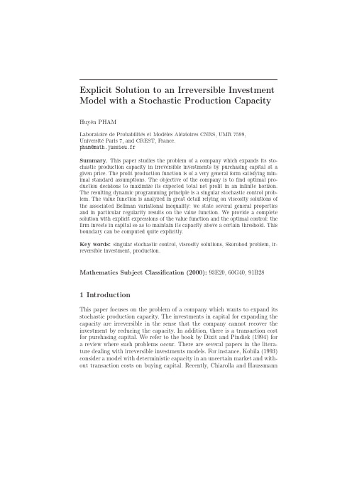
Using Soft CSPs for Approximating Pareto-Optimal Solution SetsMarc Torrens and Boi FaltingsSwiss Federal Institute of Technology(EPFL),Lausanne,SwitzerlandMarc.Torrens@epfl.ch,Boi.Faltings@epfl.chAbstractWe consider constraint satisfaction problems where so-lutions must be optimized according to multiple crite-ria.When the relative importance of different criteriacannot be quantified,there is no single optimal solution,but a possibly very large set of Pareto-optimal solutions.Computing this set completely is in general very costlyand often infeasible in practical applications.We consider several methods that apply algorithms forsoft CSP to this problem.We report on experiments,both on random and real problems,that show that suchalgorithms can compute surprisingly good approxima-tions of the Pareto-optimal set.We also derive variantsthat further improve the performance.IntroductionConstraint Satisfaction Problems(CSPs)(Tsang1993;Ku-mar1992)are ubiquitous in applications like configuration,planning,resource allocation,scheduling,timetabling andmany others.A CSP is specified by a set of variables and aset of constraints among them.A solution to a CSP is a setof value assignments to all variables such that all constraintsare satisfied.In many applications of constraint satisfaction,the objec-tive is not only tofind a solution satisfying the constraints,but also to optimize one or more preference criteria.Suchproblems occur in resource allocation,scheduling and con-figuration.As an example,we consider in particular elec-tronic catalogs with configuration functionalities:a hard constraint satisfaction problem defines the avail-able product configurations,for example different fea-tures of a PC.the customer has different preference criteria that need tobe optimized,for example price,certain functions,speed,etc.More precisely,we assume that optimization criteria aremodeled as functions that map each solution into a numer-ical value that indicates to what extent the criterion is vio-lated;i.e.the lower the value,the better the solution.1MAX-SOFT is a maximum value for soft constraints.By usinga specific maximum valuation for soft constraints,we can easilydifferenciate between a hard violation and soft violation.4) Figure1:Example of solutions in a CSP with two preference cri-teria.The two coordinates show the values indicating the degrees to which criteria(horizontal)and(vertical)are violated.and two solutions and of:and dominatesThe idea of Pareto-optimality(Pareto18961987)is to consider all solutions which are not dominated by another one as potentially optimal:Definition3.Any solution which is not dominated by an-other is called Pareto-optimal.Definition4.Given a MCOP,the Pareto-optimal set2is the set of solutions which are not dominated by any other one.In Figure1,the Pareto-optimal set is,as solu-tion7is dominated by4and6,5is dominated by3and4, and2is dominated by1.Pareto-optimal solutions are hard to compute because un-less preference criteria involve only few of the variables,the dominance relation can not be evaluated on partial solutions. Research on better algorithms for Pareto-optimality is still ongoing(see,for example,Gavanelli(Gavanelli2002)),but since it cannot escape this fundamental limitation,generat-ing all Pareto-optimal solutions is likely to always remain computationally very hard.Therefore,Pareto-optimality has so far found little use in practice,despite the fact that it characterizes optimality in a more realistic way.This is especially true when the Pareto-optimal set must be computed very quickly,for example in interactive configuration applications(e.g.electronic cata-logs).Another characteristic of the Pareto-optimal set is that it usually contains many solutions;in fact,all solutions could be Pareto-optimal.Thus,it will be necessary to have the endelectronic catalogs return a list of possibilities thatfit the criteria in decreasing degree.In general,these solutions have been calculated assuming a certain weight distribution among constraints.It appears that listing a multitude of nearly optimal solutions is intended to compensate for the fact that these weights,and thus the optimality criterion,are usually not accurate for the particular user.For example,in Figure1,if we assume that constraints have equal weight,the order of solutions would be,and the top four according to this weighting are also the Pareto-optimal ones.The questions we address in this paper follow from this observation:how closely do the top-ranked solutions generated by a scheme with known constraint weights,in particular MAX-CSP,approximate the Pareto-optimal set,and can we derive variations that cover this set better while maintaining efficiency?We have performed experiments in the domain of config-uration problems that indicate that MAX-CSP can indeed provide a surprisingly close approximation of the Pareto-optimal set both in real settings and in randomly gener-ated problems,and derive improvements to the methods that could be applied in general settings.Using Soft CSP Algorithms for ApproximatingPareto-optimal SetsTo approximate the set of Pareto-optimal solutions,the sim-plest solution is to simply map the MCOP into an opti-mization problem with a single criterion obtained by afixed weighting of the different criteria,called a weighted con-strained optimization problem(WCOP):Definition5.A WCOP is an MCOP with an associated weight vector,.The optimal solution to a COP is a tuple that minimizes the valuation functionThe best solutions to a WCOP is the set of the solutions with the lowest cost.is called the valuation of.We call feasible solutions to a WCOP those solutions which do not violate any hard constraint.Note that when the weight vector consists of all1s, WCOP is equivalent to MAX-CSP and is also an instanti-ation of the semiring CSP framework.WCOP can be solved by branch-and-bound search algorithms.These algorithms can be easily adapted to return not only the best solution,but an ordered list of the best solutions.In our work we use Partial Forward Checking(Freuder&Wallace1992)(PFC), which is a branch and bound algorithm with propagation. Pareto-optimality of WCOP SolutionsAs mentioned before,in practice it turns out that among the best solutions to a WCOP,many are also Pareto-optimal.Theorem1shows indeed that the optimal solution of a WCOP is always Pareto-optimal,and that furthermore among the best solutions all those which are not dominated by another one are Pareto-optimal for the whole problem: Theorem1.Let be the set of the best solutions ob-tained by optimizing with weights.If and is not dominated by anythen is Pareto-optimal.Proof.Assume that is not Pareto-optimal.Then,there is a solution which dominates solution,and by Definition2:andAs a consequence,we also have:i.e.must be better than according to the weighted optimization function.But this contradicts the fact that .This justifies the use of soft CSP tofind not just one,but a larger set of Pareto-optimal solutions.In particular,by filtering the best solutions returned by a WCOP algorithm to eliminate the ones which are dominated by another one in the set,wefind only solutions which are Pareto-optimal for the entire problem.We can thus bypass the costly step of proving non-dominance on the entire solution set.Thefirst algorithm is thus tofind a subset of the Pareto set by modeling it as a WCOP with a single weight vector, generating the best solutions,andfiltering them to retain only those which are not dominated(Algorithm1).Input::MCOP.:the maximal number of solutions to com-pute.Output::an approximation of the Pareto-optimal set.PFC(WCOP(P,),)eliminateDominatedSolutions()Input::MCOP.:the maximal number of solutions to com-pute.:is a collection of weight vectors.Output::an approximation of the Pareto-optimal set.PFC(WCOP(P,),) foreach doiterations,one for each cuple of constraints.The iteration for the constraints and,is performed with the weight vector,where,and .Method5:Algorithm2with100020003000400050006000700080003456789101112n u m b e r o f p a r e t o o p t i m a l s o l u t i o n snumber of criteria (soft constraints)Random problem with n=5, d=10, hc=20%hard tightness = 20%hard tightness = 40%hard tightness = 60%hard tightness = 80%Figure 2:Number of Pareto-optimal solutions depending on how many soft constraints we consider for random generated problems with 5variables,10values per domain and 20%of hard unary/binary constraint density.The number of of solutions in average for the generated problems are:for hard tightness =20%,for hard tightness =40%,for hard tightness =60%and 778for hard tightness =80%.number of criteria (soft constraints).In Figure 2,it is shown that the number of Pareto-optimal solutions clearly increases when the number of criteria increases.The same phenom-ena applies for instances with 5and 10variables.On the other hand,we have observed that even if the number of Pareto-optimal solutions decreases when the problem gets more constrained (less feasible solutions)the percentage in respect to the total number of solutions increases.Thus,the proportion of the Pareto-optimal solutions is more important when the problem gets more constrained.We have evaluated the proposed methods for each type of generated problems.Figure 3shows the proportion in avarage of Pareto-optimal solutions found by the different methods for problems with 6soft constrains.We emphasize the results of the methods up to 530solutions because in real applications it could not be feasible to compute a largerset of solutions.When computing up tosolutions,the behavior of the different methods does not change sig-nificantly.The 50randomly generated problems used for Figure 3had in avarage feasible solutions (satisfy-ing hard constraints)andPareto-optimal solutions.The iterative methods perform better than the single search al-gorithm (Method 1)in respect to the total number of solu-tions computed.It is worth to note that the iterative meth-ods based on Algorithm 2find more Pareto-optimal solu-tions when the number of iterations increase.Lexicographic Fuzzy method (Method 6)results in finding a very low per-centage of Pareto-optimal solutions (less than ).With Method 6,Theorem 1does not apply,thus the percentage shown of Pareto-optimal solutions is computed a posteriori by filtering out the Pareto-optimal solutions that were not really Pareto-optimal for the entire problem.Another way of comparing the different methods is to% o f P a r e t o o p t i m a l s o l u t i o n s f o u n dTotal number of computed solutionsEvaluation of different methodsFigure 3:Pareto-optimal solutions found by the different proposed methods (in %).Methods are applied to 50ran-domly generated problems with 10variables,10values per domain,40%of density of hard unary/binary constraints with 40%of hard tightness and 6criteria (soft constraints).The number of total computed solutions for each method varies from 30to 530in steps of 100.% o f P a r e t o o p t i m a l s o l u t i o n s f o u n dTime in secondsEvaluation of different methodsFigure 4:Number of Pareto-optimal solutions found by the different proposed methods with respect to the computing time.For this plot,the problems have 10variables,10values per domain with 40%of hard unary/binary constraints with 40%of hard tightness and 6criteria (soft constraints).compare the number of Pareto-optimal solutions found withrespect to the computing time(Figure4).Using this com-parison,Method1performs the best.The performance ofthe variants of Method2decreases when the number of it-erations increases.Method3performs better than method4 which performs better than method5in terms of computingtime.In general,we can observe that when the number of it-erations of the methods increases the performance regardingthe total number of computed solutions also increases but theperformance regarding the computing time decreases.This is due to the fact that the computing time offinding the bestsolutions with PFC is not linear with respect offinding the best solutions with iterations(solutions per itera-tion).For example,computing solutions with one it-eration takes seconds and computing solutionswith7iterations(of solutions)takes seconds.Even if the tests based on Algorithm2takes more timethan Algorithm1for getting the same percentage of Pareto-optimal solutions,they are likely to produce a more repre-sentative set of the Pareto-optimal set.Using a brute force algorithm that computes all the feasi-ble solutions andfilter out those which are dominated took inavarage seconds for the same problems as in the above figures.This demonstrates the interest of using approxima-tive methods for computing Pareto-optimal solutions,espe-cially for interactive configuration applications(e.g.elec-tronic catalogs).Empirical Results in a Real Application The Air Travel ConfiguratorThe problem of arranging trips is here modeled as a softCSP(see(Torrens,Faltings,&Pu2002)for a detailed de-scription of our travel configurator).An itinerary is a set of legs,where each leg is represented by a set of origins,a set of destinations,and a set of possible dates.Leg variables represent the legs of the itinerary and their domains are the possibleflights for the associated leg.Another variable rep-resents the set of possible fares3applicable to the itinerary. The same itinerary can have several different fares depend-ing on the cabin class,airline,schedule and so u-ally,for each leg there can be about60flights,and for each itinerary,there can be about40fares.Therefore,the size of the search space for a round trip is and for a three leg trip is.Constraint sat-isfaction techniques are well-suited for modeling the travel planning problem.In our model,two types of configuration constraints(hard constraints)guarantee that:1.aflight for a leg arrives before aflight for a legtakes off,and2.a fare can be really applicable to a set offlights(depend-ing on the fare rules).Users normally have preferences about the itinerary they are willing to plan.They can have preferences about the schedule of the itinerary,the airlines,the class of service,tofind a certain number of Pareto-optimal solutions,even if this set only represents a small fraction of all the Pareto-optimal solutions.Actually,we consider that the number of total solutions that can be shown to the user must be small because of the limitations of the current graphical user inter-faces.Related WorkThe most commonly used approach for solving a Multi-criteria Optimization Problem is to convert a MCOP into several COPs which can be solved using standard mono-criteria optimization techniques.Each COP will give then a Pareto-optimal solution to the problem.Steuer’s book(Steuer1986)gives a deep study on different ways to translate a MCOP to a set of COPs.The most used strategy is to optimize by one linear function of all crite-ria with positive weights.The drawback of the method is that some Pareto-optimal solutions cannot be found if the efficient frontier is not concave4.Our methods are based on this approach.Gavanelli(Gavanelli2002;2001)addresses the problem of multi-critera optimization in constraint problems directly. His method is based in a branch and bound schema where the Paerto dominance is checked against a set of previously found solutions using Point Quad-Trees.Point Quad-Trees are useful for efficiently bounding the search.However,the algorithm can be very costly if the number of criteria or if the number of Pareto-optimal solutions are high.Gavanelli’s method significantly improves the approach of Wassenhove-Geders(Wassenhove&Gelders1980).The Wassenhove-Geder’s method basically consists of performing several search processes,one for each criteria.Each iteration takes the previous solution and tries to improve it by optimizing another ing this method,each search produces one Pareto-optimal solution,so a lot of search process must be done in order to approximate the Pareto-optimal set. The Global Criterion Method tries to solve a MCOP as a COP where the criteria to optimize is a minimization func-tion of a distance function to an ideal solution.The ideal solution is precomputed by optimizing each criteria inde-pendently(Salukvadze1974).Incomplete methods have also been developed for solving multi-criteria optimization,basically:genetic algorithms(Deb1999)and methods based on tabu search(Hansen1997).ConclusionsThis paper deals with a very well-studied topic,Pareto-optimality in multi-criteria optimization.It has been com-monly understood that Pareto-optimality is intractable to compute,and therefore has not been studied further.In-stead,many applications have simply mapped multi-criteria search into a single criterion with a particular weighting and returned a list of the best solutions rather than a single best one.This solution allows leveraging the well-developedKumar,V.1992.Algorithms for Constraint Satisfaction Problems:A Survey.AI Magazine13(1):32–44. Pareto,V.1896-1987.Cours d’´e conomie politique profess´e `a l’universit´e de Lausanne,usanne:F.Rouge. Salukvadze,M.E.1974.On the existence of solu-tion in problems of optimization under vector valued cri-teria.Journal of Optimization Theory and Applications 12(2):203–217.Steuer,R.E.1986.Multi Criteria Optimization:Theory, Computation,and Application.New York:Wiley. Torrens,M.;Faltings,B.;and Pu,P.2002.Smartclients: Constraint satisfaction as a paradigm for scaleable intel-ligent information systems.CONSTRAINTS:an interna-tional journal7:49–69.Tsang,E.1993.Foundations of Constraint Satisfaction. London,UK:Academic Press.Wassenhove,L.N.V.,and Gelders,L.F.1980.Solving a bicriterion scheduling problem.European Journal of Op-erational Research4(1):42–48.。