R. Hartley Self-cal.ibration from multiple views with a rotating camera

Reference: 1. M. Turk and A. Pentland, "Eigenfaces for recognition", J. of Cognitive Neuroscience, Vol. 3, No. 1, pp. 71-86, 1991. 2. M. Turk and B. Moghaddam, and T. Starner, “View-based and modular eigenspaces for face recognition", Proc. of CVPR, pp. 21-23, 1994.
Introduction
Identification
– When an unknown face is input, the system determines the identity through a one-to-many matching with all the known individuals in the database.
Let the a set of training face images be represented by a X x , , x N by M matrix: 1 M N: the number of pixels in images; M: image number
T C xi mxi m
Face Recognition
[name]
Outline
Introduction Difficulties for face recognition Methods
– Feature based face recognition – Appearance based face recognition – Elastic Bunch Graph Matching Face Database

Initial parameters
Calibration settings 'pose' 'params' …
CalibModelID
Observed points
Calibration result
Data gathering and parameter setup are handled by flexible operators
set_calib_data_observ_points (:: ► CalibDataID, ► CameraIndex, ► CalibObjIndex, ► CalibObjPoseIndex, ► Row, Column, 0 ► Index, ► Pose :)
1 2
0
3
1
Configure optimization parameters
Planare about object geometry?
Yes
Feature points
Vector to pose
No 3D object model
Planar
3D reconstruction
Primitive fitting
CAD model
Yes
Unknown
Multi-view Stereo
Sheet-of-light technique
Select Your Solution: Planar
Geometric primitives?
No Clear edges?
Yes
Perspective, deformable matching
Configuration Create model create_calib_data

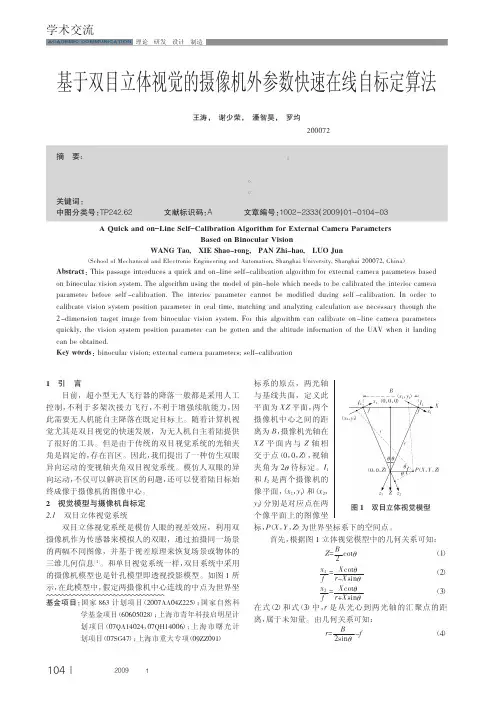
基金项目：国家863计划项目（2007AA04Z225）；国家自然科学基金项目（60605028）；上海市青年科技启明星计划项目（07QA14024，07QH14006）；上海市曙光计划项目（07SG47）；上海市重大专项（09ZZ091）!!!!!!!!!!!!!!!!基于双目立体视觉的摄像机外参数快速在线自标定算法王涛，谢少荣，潘智昊，罗均（上海大学机械电子工程与自动化学院，上海200072）1引言目前，超小型无人飞行器的降落一般都是采用人工控制，不利于多架次接力飞行，不利于增强续航能力，因此需要无人机能自主降落在既定目标上。

随着计算机视觉尤其是双目视觉的快速发展，为无人机自主着陆提供了很好的工具。

但是由于传统的双目视觉系统的光轴夹角是固定的，存在盲区。

因此，我们提出了一种仿生双眼异向运动的变视轴夹角双目视觉系统。

模仿人双眼的异向运动，不仅可以解决盲区的问题，还可以使着陆目标始终成像于摄像机的图像中心。

2视觉模型与摄像机自标定2.1双目立体视觉系统双目立体视觉系统是模仿人眼的视差效应，利用双摄像机作为传感器来模拟人的双眼，通过拍摄同一场景的两幅不同图像，并基于视差原理来恢复场景或物体的三维几何信息［1］。

和单目视觉系统一样，双目系统中采用的摄像机模型也是针孔模型即透视投影模型。

如图1所示，在此模型中，假定两摄像机中心连线的中点为世界坐标系的原点，两光轴与基线共面，定义此平面为XZ 平面，两个摄像机中心之间的距离为B ，摄像机光轴在XZ 平面内与Z 轴相交于点（0，0，Z ），视轴夹角为2θ待标定。

I 1和I 2是两个摄像机的像平面，（x 1，y 1）和（x 2，y 2）分别是对应点在两个像平面上的图像坐标，P （X ，Y ，Z ）为世界坐标系下的空间点。

首先，根据图1立体视觉模型中的几何关系可知：Z =B 2cot θ（１）x 1=X cot θ（２）x 2f =X cot θr+X sin θ（3）在式（2）和式（3）中，r 是从光心到两光轴的汇聚点的距离，属于未知量。

Single-Pixel Imaging via Compressive SamplingMarco F.Duarte,Mark A.Davenport,Dharmpal Takhar,Jason skaTing Sun,Kevin F.Kelly,Richard G.BaraniukRice UniversityHumans are visual animals,and imaging sensors that extend our reach–cameras–have improved dramatically in recent times thanks to the introduction of CCD and CMOS digital technology.Consumer digital cameras in the mega-pixel range are now ubiquitous thanks to the happy coincidence that the semiconductor material of choice for large-scale electronics integration (silicon)also happens to readily convert photons at visual wavelengths into electrons.On the contrary,imaging at wavelengths where silicon is blind is considerably more complicated,bulky, and expensive.Thus,for comparable resolution,a$500digital camera for the visible becomes a $50,000camera for the infrared.In this paper,we present a new approach to building simpler,smaller,and cheaper digital cameras that can operate efficiently across a much broader spectral range than conventional silicon-based cameras.Our approach fuses a new camera architecture based on a digital mi-cromirror device(DMD–see Sidebar:Spatial Light Modulators)with the new mathematical theory and algorithms of compressive sampling(CS–see Sidebar:Compressive Sampling in a Nutshell).CS combines sampling and compression into a single nonadaptive linear measurement process [1–4].Rather than measuring pixel samples of the scene under view,we measure inner products between the scene and a set of test functions.Interestingly,random test functions play a key role, making each measurement a random sum of pixel values taken across the entire image.When the scene under view is compressible by an algorithm like JPEG or JPEG2000,the CS theory enables us to stably reconstruct an image of the scene from fewer measurements than the number of reconstructed pixels.In this manner we achieve sub-Nyquist image acquisition.Our“single-pixel”CS camera architecture is basically an optical computer(comprising a DMD,two lenses,a single photon detector,and an analog-to-digital(A/D)converter)that computes random linear measurements of the scene under view.The image is then recovered orFig.1.Aerial view of the single-pixel compressive sampling(CS)camera in the lab[5].processed from the measurements by a digital computer.The camera design reduces the required size,complexity,and cost of the photon detector array down to a single unit,which enables the use of exotic detectors that would be impossible in a conventional digital camera.The random CS measurements also enable a tradeoff between space and time during image acquisition.Finally, since the camera compresses as it images,it has the capability to efficiently and scalably handle high-dimensional data sets from applications like video and hyperspectral imaging.This article is organized as follows.After describing the hardware,theory,and algorithms of the single-pixel camera in detail,we analyze its theoretical and practical performance and compare it to more conventional cameras based on pixel arrays and raster scanning.We also explain how the camera is information scalable in that its random measurements can be used to directly perform simple image processing tasks,such as target classification,withoutfirst reconstructing the underlying imagery.We conclude with a review of related camera architectures and a discussion of ongoing and future work.I.The Single-Pixel CameraArchitectureThe single-pixel camera is an optical computer that sequentially measures the inner products y[m]= x,φm between an N-pixel sampled version x of the incident light-field from the scene under view and a set of two-dimensional(2D)test functions{φm}[5].As shown in Fig.1,thelight-field is focused by biconvex Lens1not onto a CCD or CMOS sampling array but rather onto a DMD consisting of an array of N tiny mirrors(see Sidebar:Spatial Light Modulators).Each mirror corresponds to a particular pixel in x andφm and can be independently oriented either towards Lens2(corresponding to a1at that pixel inφm)or away from Lens2(corre-sponding to a0at that pixel inφm).The reflected light is then collected by biconvex Lens2and focused onto a single photon detector(the single pixel)that integrates the product x[n]φm[n]to compute the measurement y[m]= x,φm as its output voltage.This voltage is then digitized by an A/D converter.Values ofφm between0and1can be obtained by dithering the mirrors back and forth during the photodiode integration time.To obtainφm with both positive and negative values(±1,for example),we estimate and subtract the mean light intensity from each measurement,which is easily measured by setting all mirrors to the full-on1position.To compute CS randomized measurements y=Φx as in(1),we set the mirror orientations φm randomly using a pseudo-random number generator,measure y[m],and then repeat the process M times to obtain the measurement vector y.Recall from Sidebar:Compressive Sampling in a Nutshell that we can set M=O(K log(N/K))which is≪N when the scene being imaged is compressible by a compression algorithm like JPEG or JPEG2000.Since the DMD array is programmable,we can also employ test functionsφm drawn randomly from a fast transform such as a Walsh,Hadamard,or Noiselet transform[6,7].The single-pixel design reduces the required size,complexity,and cost of the photon detector array down to a single unit,which enables the use of exotic detectors that would be impossible in a conventional digital camera.Example detectors include a photomultiplier tube or an avalanche photodiode for low-light(photon-limited)imaging(more on this below),a sandwich of several photodiodes sensitive to different light wavelengths for multimodal sensing,a spectrometer for hyperspectral imaging,and so on.In addition to sensingflexibility,the practical advantages of the single-pixel design include the facts that the quantum efficiency of a photodiode is higher than that of the pixel sensors in a typical CCD or CMOS array and that thefill factor of a DMD can reach90%whereas that of a CCD/CMOS array is only about50%.An important advantage to highlight is the fact that each CS measurement receives about N/2times more photons than an average pixel sensor,which significantly reduces image distortion from dark noise and read-out noise.Theoretical advantages(a)(b)(c)Fig.2.Single-pixel photo album.(a)256×256conventional image of a black-and-white R.(b)Single-pixel camera reconstructed image from M=1300random measurements(50×sub-Nyquist).(c)256×256 pixel color reconstruction of a printout of the Mandrill test image imaged in a low-light setting using a single photomultiplier tube sensor,RGB colorfilters,and M=6500random measurements.that the design inherits from the CS theory include its universality,robustness,and progressivity.The single-pixel design falls into the class of multiplex cameras[8].The baseline standard for multiplexing is classical raster scanning,where the test functions{φm}are a sequence of delta functionsδ[n−m]that turn on each mirror in turn.As we will see below,there are substantial advantages to operating in a CS rather than raster scan mode,including fewer total measurements (M for CS rather than N for raster scan)and significantly reduced dark noise.Image acquisition examplesFigure2(a)and(b)illustrates a target object(a black-and-white printout of an“R”)x and reconstructed image x taken by the single-pixel camera prototype in Fig.1using N=256×256 and M=N/50[5].Fig.2(c)illustrates an N=256×256color single-pixel photograph of a printout of the Mandrill test image taken under low-light conditions using RGB colorfilters and a photomultiplier tube with M=N/10.In both cases,the images were reconstructed using Total Variation minimization,which is closely related to wavelet coefficientℓ1minimization[2].Structured illumination configurationIn a reciprocal configuration to that in Fig.1,we can illuminate the scene using a projector displaying a sequence of random patterns{φm}and collect the reflected light using a single lens and photodetector.Such a“structured illumination”setup has advantages in applications where we can control the light source.In particular,there are intriguing possible combinations of single-pixel imaging with techniques such as3D imaging and dual photography[9].Shutterless video imagingWe can also acquire video sequences using the single-pixel camera.Recall that a traditional video camera opens a shutter periodically to capture a sequence of images(called video frames) that are then compressed by an algorithm like MPEG that jointly exploits their spatio-temporal redundancy.In contrast,the single-pixel video camera needs no shutter;we merely continuously sequence through randomized test functionsφm and then reconstruct a video sequence using an optimization that exploits the video’s spatio-temporal redundancy[10].If we view a video sequence as a3D space/time cube,then the test functionsφm lie concentrated along a periodic sequence of2D image slices through the cube.A na¨ıve way to reconstruct the video sequence would group the corresponding measurements y[m]into groups where the video is quasi-stationary and then perform a2D frame-by-frame reconstruction on each group.This exploits the compressibility of the3D video cube in the space but not time direction.A more powerful alternative exploits the fact that even though eachφm is testing a different 2D image slice,the image slices are often related temporally through smooth object motions in the video.Exploiting this3D compressibility in both the space and time directions and inspired by modern3D video coding techniques[11],we can,for example,attempt to reconstruct the sparsest video space/time cube in the3D wavelet domain.These two approaches are compared in the simulation study illustrated in Fig.3.We employed simplistic3D tensor product Daubechies-4wavelets in all cases.As we see from thefigure,3D reconstruction from2D random measurements performs almost as well as3D reconstruction from 3D random measurements,which are not directly implementable with the single-pixel camera.II.Single-Pixel Camera TradeoffsThe single-pixel camera is aflexible architecture to implement a range of different multiplex-ing methodologies,just one of them being CS.In this section,we analyze the performance of CS and two other candidate multiplexing methodologies and compare them to the performance of a brute-force array of N pixel sensors.Integral to our analysis is the consideration of Poisson photon counting noise at the detector,which is image-dependent.We conduct two separate analyses to assess the“bang for the buck”of CS.Thefirst is a theoretical analysis that provides general guidance.The second is an experimental study that indicates how the systems typically perform(a)frame32(b)2D meas(c)2D meas(d)3D meas+2D recon+3D recon+3D reconFig.3.Frame32from a reconstructed video sequence using(top row)M=20,000and(bottom row) M=50,000measurements(simulation from[10]).(a)Original frame of an N=64×64×64video of a disk simultaneously dilating and translating.(b)Frame-by-frame2D measurements+frame-by-frame 2D reconstruction;MSE=3.63and0.82,respectively.(c)Frame-by-frame2D measurements+joint3D reconstruction;MSE=0.99and0.24,respectively.(d)Joint3D measurements+joint3D reconstruction; MSE=0.76and0.18,respectively.in practice.Scanning methodologiesThe four imaging methodologies we consider are:•Pixel array(PA):a separate sensor for each of the N pixels receives light throughout the total capture time T.This is actually not a multiplexing system,but we use it as the gold standard for comparison.•Raster scan(RS):a single sensor takes N light measurements sequentially from each of the N pixels over the capture time.This corresponds to test functions{φm}that are delta functions and thusΦ=I.The measurements y thus directly provide the acquired image x.•Basis scan(BS):a single sensor takes N light measurements sequentially from different combinations of the N pixels as determined by test functions{φm}that are not delta functions but from some more general basis[12].In our analysis,we assume a Walsh basis modified to take the values0/1rather than±1;thusΦ=W,where W is the0/1Walsh matrix.The acquired image is obtained from the measurements y by x=Φ−1y=W−1y.•Compressive sampling(CS):a single sensor takes M≤N light measurements sequentially from different combinations of the N pixels as determined by random0/1test functions {φm}.Typically,we set M=O(K log(N/K))which is≪N when the image is com-pressible.In our analysis,we assume that the M rows of the matrixΦconsist of randomlydrawn rows from a0/1Walsh matrix that are then randomly permuted(we ignore thefirst row consisting of all1’s).The acquired image is obtained from the measurements y via a sparse reconstruction algorithm such as BPIC(see Sidebar:Compressive Sampling in a Nutshell).Theoretical analysisIn this section,we conduct a theoretical performance analysis of the above four scanning methodologies in terms of the required dynamic range of the photodetector,the required bit depth of the A/D converter,and the amount of Poisson photon counting noise.Our results are pessimistic in general;we show in the next section that the average performance in practice can be considerably better.Our results are summarized in Table I.An alternative analysis of CS imaging for piecewise smooth images in Gaussian noise has been reported in[13].Dynamic range:Wefirst consider the photodetector dynamic range required to match the performance of the baseline PA.If each detector in the PA has a linear dynamic range of0to D, then it is easy to see that single-pixel RS detector need only have that same dynamic range.In contrast,each Walsh basis test function contains N/21’s,and so directs N/2times more light to the detector.Thus,BS and CS each require a larger linear dynamic range of0to ND/2.On the positive side,since BS and CS collect considerably more light per measurement than the PA and RS,they benefit from reduced detector nonidealities like dark currents.Quantization error:We now consider the number of A/D bits required within the required dynamic range to match the performance of the baseline PA in terms of worst-case quantization distortion.Define the mean-squared error(MSE)between the true image x and its acquired version x as MSE=1ND2−B−1[14].Due to its larger dynamic range,BS requires B+ log2N bits per measurement to reach the same MSE distortion level.Since the distortion of CS reconstruction is up to C N times larger than the distortion in the measurement vector(see Sidebar: Compressive Sensing in a Nutshell),we require up to an additional log2C N bits per measurement. One empirical study has found roughly that C N lies between8and10for a range of different random measurement configurations[15].Thus,BS and CS require a higher-resolution A/D converter than PA and RS to acquire an image with the same worst-case quantization distortion.TABLE IComparison of the four camera scanning methodologies.Raster Scan Compressive Sampling N ND ND NDNB N(B+log2N)P N P(3N−2)P<3C2NM P3C2N, the MSE of CS is lower than that of RS.We emphasize that in the CS case,we have only a fairly loose upper bound and that there exist alternative CS reconstruction algorithms with better performance guarantees,such as the Dantzig Selector[3].Summary:From Table I,we see that the advantages of a single-pixel camera over a PA come at the cost of more stringent demands on the sensor dynamic range and A/D quantization and larger MSE due to photon counting effects.Additionally,the linear dependence of the MSE on the number of image pixels N for BS and RS is a potential deal-breaker for high-resolution imaging.The promising aspect of CS is the logarithmic dependence of its MSE on N through the relationship M=O(K log(N/K)).Experimental resultsSince CS acquisition/reconstruction methods often perform much better in practice than the above theoretical bounds suggest,in this section we conduct a simple experiment using real data from the CS imaging testbed depicted in Fig.1.Thanks to the programmability of the testbed, we acquired RS,BS,and CS measurements from the same hardware.Wefixed the number of A/D converter bits across all methodologies.Figure4shows the pixel-wise MSE for the capture of a N=128×128pixel“R”test image as a function of the total capture time T.Here the MSE combines both quantization and photon counting effects.For CS we took M=N/10total measurements per capture and used a Daubechies-4wavelet basis for the sparse reconstruction.We make two observations.First,the performance gain of BS over RS contradicts the aboveFig.4.Average MSE for Raster Scan(RS),Basis Scan(BS),and Compressive Sampling(CS)single-pixel images as a function of the total image capture time T(real data).worst-case theoretical calculations.We speculate that the contribution of the sensor’s dark current, which is not accounted for in our analysis,severely degrades RS’s performance.Second,the performance gain of CS over both RS and BS is clear:images can either be acquired in much less time for the same MSE or with much lower MSE in the same amount of time.rmation Scalability and the Smashed FilterWhile the CS literature has focused almost exclusively on problems in signal and image reconstruction or approximation,reconstruction is frequently not the ultimate goal.For instance, in many image processing and computer vision applications,data is acquired only for the purpose of making a detection,classification,or recognition decision.Fortunately,the CS framework is information scalable to a much wider range of statistical inference tasks[17–19].Tasks such as detection do not require reconstruction,but only require estimates of the relevant sufficient statistics for the problem at hand.Moreover,in many cases it is possible to directly extract these statistics from a small number of random measurements without ever reconstructing the image.The matchedfilter is a key tool in detection and classification problems that involve searching for a target template in a scene.A complicating factor is that often the target is transformed in some parametric way—for example the time or Doppler shift of a radar return signal;the translation and rotation of a face in a face recognition task;or the roll,pitch,yaw,and scale of a vehicle viewed from an aircraft.The matchedfilter detector operates by forming comparisons between the given test data and all possible transformations of the template tofind the match that optimizes some performance metric.The matchedfilter classifier operates in the same waybut chooses the best match from a number of different potential transformed templates.The na¨ıve approach to matchedfiltering with CS wouldfirst reconstruct the images under consideration and then apply a standard matchedfiltering technique.In contrast,the smashed filter(for dimensionally reduced matchedfilter)performs all of its operations directly on the random measurements[18].The two key elements of the smashedfilter are the generalized likelihood ratio test and the concept of an image appearance manifold[20].If the parametric transformation affecting the template image is well-behaved,then the set of transformed templates forms a low-dimensional manifold in the high-dimensional pixel space R N with the dimension K equal to the number of independent parameters.1Thus,the matchedfilter classifier can be interpreted as classifying a test image according to the closest template manifold in R N.The smashedfilter exploits a recent result that the structure of a smooth K-dimensional manifold in R N is preserved with high probability under a random projection to the lower dimensional space R M as long as M=O(K log N)[21].This is reminiscent of the number of measurements required for successful CS but with K now the manifold dimension.Thus,to classify an N-pixel test image,we can alternatively compare M random measurements of the test image to the M-dimensional projections(using the sameΦ)of the candidate image template manifolds.The upshot is that all necessary computations can be made directly in R M rather than in R N.As in the conventional matchedfilter,a byproduct of the closest manifold search is an estimate of the template parameters that best match the test image.Previous work in the computer science community(the other“CS”)has also employed the Johnson-Lindenstrauss lemma[22] to reduce the data dimensionality prior to computing features for classification;however,they have not considered the intrinsic manifold structure manifested in many image processing and computer vision settings.Figure5demonstrates the effectiveness of smashedfiltering for the task of classifying an N= 128×128pixel test image under an unknown translation in the vertical and horizontal directions (hence K=2).The three classes correspond to different translations of a bus,truck,or tank.The test data was generated randomly from one of the three classes.The random measurements were 1For the purposes of the discussion here,a K-dimensional manifold can be interpreted as a K-dimensional hypersurface in R N.Fig.5.Smashedfilter image classification performance plotted as a function of the number of random measurements M from a simulated single-pixel CS camera and the total acquisition time T.produced using a simulated single-pixel CS camera that takes into account the Poisson photon counting noise associated with a total measurement interval of length T.We average over10,000 iterations of each experiment.We see that increasing the number of measurements improves performance atfirst;however,performance then degrades due to the reduced time available to obtain each measurement.Correspondingly,increasing the total capture time improves the performance of the algorithm.IV.Other Multiplexing Camera ArchitecturesTwo notable existing DMD-driven imaging applications involve confocal microscopy(which relates closely to the raster scan strategy studied above)[23,24]and micro-optoelectromechanical (MOEM)systems[12,25,26].In a MOEM system,a DMD is positioned between the scene and the sensing array to perform column-wise multiplexing by allowing only the light from the desired pixels to pass through.In[12,25]the authors propose sets of N Hadamard patterns,which enables simple demultiplexing,and randomized Hadamard patterns,which yield a uniform signal-to-noise ratio among the measurements.Other compressive cameras developed to date include[27,28],which employ optical elements to perform transform coding of multispectral images.These designs obtain sampled outputs that correspond to coded information of interest,such as the wavelength of a given light signal or the transform coefficients in a basis of interest.The elegant hardware designed for these purposes uses optical projections,group testing,and signal inference.Recent work in[29]has compared several single and multiple pixel imaging strategies of varying complexities;their simulationresults for Poisson counting noise agree closely with those above.Finally,in[30]the authors use CS principles and a randomizing lens to boost both the resolution and robustness of a conventional digital camera.V.ConclusionsFor certain applications,CS promises to substantially increase the performance and capabil-ities of data acquisition,processing,and fusion systems while lowering the cost and complexity of deployment.A useful practical feature of the CS approach is that it off-loads processing from data acquisition(which can be complicated and expensive)into data reconstruction or processing (which can be performed on a digital computer,perhaps not even co-located with the sensor).We have presented an overview of the theory and practice of a simple yetflexible single-pixel architecture for CS based on a DMD spatial light modulator.While there are promising potential applications where current digital cameras have difficulty imaging,there are clear tradeoffs and challenges in the single-pixel design.Our current and planned work involves better understanding and addressing these tradeoffs and challenges.Other potential avenues for research include extending the single-pixel concept to wavelengths where the DMD fails as a modulator,such as THz and X-rays.Sidebar:Compressive Sampling in a NutshellCompressive Sampling(CS)is based on the recent understanding that a small collection of nonadaptive linear measurements of a compressible signal or image contain enough information for reconstruction and processing[1–3].For a tutorial treatment see[4]or the paper by Romberg in this issue.The traditional approach to digital data acquisition samples an analog signal uniformly at or above the Nyquist rate.In a digital camera,the samples are obtained by a2D array of N pixel sensors on a CCD or CMOS imaging chip.We represent these samples using the vector x with elements x[n],n=1,2,...,N.Since N is often very large,e.g.in the millions for today’s consumer digital cameras,the raw image data x is often compressed in the following multi-step transform coding process.Thefirst step in transform coding represents the image in terms of the coefficients{αi}of an orthonormal basis expansion x= N i=1αiψi where{ψi}N i=1are the N×1basis vectors.Forming the coefficient vectorαand the N×N basis matrixΨ:=[ψ1|ψ2|...|ψN]by stacking the vectors{ψi}as columns,we can concisely write the samples as x=Ψα.The aim is to find a basis where the coefficient vectorαis sparse(where only K≪N coefficients arenonzero)or r-compressible(where the coefficient magnitudes decay under a power law withscaling exponent−r).For example,natural images tend to be compressible in the discrete cosinetransform(DCT)and wavelet bases on which the JPEG and JPEG-2000compression standardsare based.The second step in transform coding encodes only the values and locations of the Ksignificant coefficients and discards the rest.This sample-then-compress framework suffers from three inherent inefficiencies:First,wemust start with a potentially large number of samples N even if the ultimate desired K is small.Second,the encoder must compute all of the N transform coefficients{αi},even though it will discard all but K of them.Third,the encoder faces the overhead of encoding the locations of the large coefficients.As an alternative,CS bypasses the sampling process and directly acquires a condensedrepresentation using M<N linear measurements between x and a collection of test functions{φm}M m=1as in y[m]= x,φm .Stacking the measurements y[m]into the M×1vector y and the test functionsφT m as rows into an M×N matrixΦwe can writey=Φx=ΦΨα.(1)The measurement process is non-adaptive in thatΦdoes not depend in any way on the signal x.The transformation from x to y is a dimensionality reduction and so loses information in general.In particular,since M<N,given y there are infinitely many x′such thatΦx′=y. The magic of CS is thatΦcan be designed such that sparse/compressible x can be recovered exactly/approximately from the measurements y.While the design ofΦis beyond the scope of this review,an intriguing choice that works with high probability is a random matrix.For example,we can draw the elements ofΦas independent and identically distributed(i.i.d.)±1random variables from a uniform Bernoulli distribution[22]. Then,the measurements y are merely M different randomly signed linear combinations of the elements of x.Other possible choices include i.i.d.,zero-mean,1/N-variance Gaussian entries (white noise)[1–3,22],randomly permuted vectors from standard orthonormal bases,or random。