6-2-分子动力学简介

分子动力学综述分子动力学模拟方法综述（电子科技大学，微电子与固体电子学院，刘家豪）摘要：任何物质从微观的角度去看，都是由原子分子或者离子构成。

这些原子，分子或离子之间的相互作用，它们之间的关系直接决定了由此原子组成的宏观物质的各种参数，包括热传导性，温度，压力，粘性等等。

随着现代计算机技术的发展，利用统计物理学的知识，分子动力学（Molecular Dynamics）模拟方法已经成为现代科研过程中除理论研究，实验研究之外的第三种有效科研手段，自1957年发展至今，分子动力学（MD）已经广泛应用于物理，化学，生物，材料等各个学科之中。

什么是分子动力学，分子动力学就是利用计算机技术，对由原子核，电子所构成的多体系的整个运动过程进行模拟，从而实时将分子的行为显示在计算机屏幕上，进而从理论上得出宏观物体的各种性质。

本文将从理论角度出发简要论述分子动力学模拟方法。

关键字：分子动力学，势能函数，势能模型一．分子动力学基本原则：1.各个原子，分子遵循经典牛顿力学定律：在经典分子动力学模拟方法中，忽略了电子的作用，因此忽略了量子效应，同时各个原子满足牛顿运动学方程满足叠加定理，所以可以使用经典物理学的手段去处理原子的运动问题。

2.适用范围：经典的分子动力学模拟只考虑了多体系统中的原子核，忽略了量子效应，这种忽略对于很多经典的材料是十分适用的，当我们要考虑原子核的转动，平动或者频率的时候，才考虑量子效应。

3.前提，假设：已知微观粒子的相互作用。

分子为球形，之间的相互作用只由其之间的距离决定。

、二．分子动力学模拟主要步骤：1.选取要研究的系统与其边界，根据实际需求建立合理的势能模型：1.1系统：在分子动力学中所研究的系统主要有三种：（1）微正则系宗（NET）：微正则系宗为孤立系统，系统内的原子数，能量，体积等参数不随时间发生改变。

（2）正则系宗（NVT）：在正则系宗里，系统的原子数，体积，温度不发生改变，同时系统的总动量为零。

第六章 分子动力学方法6.1引言对于一个多粒子体系的实验观测物理量的数值可以由总的平均得到。

但是由于实验体系又非常大，我们不可能计算求得所有涉及到的态的物理量数值的总平均。

按照产生位形变化的方法，我们有两类方法对有限的一系列态的物理量做统计平均：第一类是随机模拟方法。

它是实现Gibbs的统计力学途径。

在此方法中，体系位形的转变是通过马尔科夫(Markov)过程，由随机性的演化引起的。

这里的马尔科夫过程相当于是内禀动力学在概率方面的对应物。

该方法可以被用到没有任何内禀动力学模型体系的模拟上。

随机模拟方法计算的程序简单，占内存少，但是该方法难于处理非平衡态的问题。

另一类为确定性模拟方法，即统计物理中的所谓分子动力学方法（Molecular Dynamics Method）。

这种方法广泛地用于研究经典的多粒子体系的研究中。

该方法是按该体系内部的内禀动力学规律来计算并确定位形的转变。

它首先需要建立一组分子的运动方程，并通过直接对系统中的一个个分子运动方程进行数值求解，得到每个时刻各个分子的坐标与动量，即在相空间的运动轨迹，再利用统计计算方法得到多体系统的静态和动态特性, 从而得到系统的宏观性质。

因此，分子动力学模拟方法可以看作是体系在一段时间内的发展过程的模拟。

在这样的处理过程中我们可以看出：分子动力学方法中不存在任何随机因素。

系统的动力学机制决定运动方程的形式：在分子动力学方法处理过程中，方程组的建立是通过对物理体系的微观数学描述给出的。

在这个微观的物理体系中，每个分子都各自服从经典的牛顿力学。

每个分子运动的内禀动力学是用理论力学上的哈密顿量或者拉格朗日量来描述，也可以直接用牛顿运动方程来描述。

这种方法可以处理与时间有关的过程，因而可以处理非平衡态问题。

但是使用该方法的程序较复杂，计算量大，占内存也多。

适用范围广泛：原则上，分子动力学方法所适用的微观物理体系并无什么限制。

这个方法适用的体系既可以是少体系统，也可以是多体系统；既可以是点粒子体系，也可以是具有内部结构的体系；处理的微观客体既可以是分子，也可以是其它的微观粒子。

分子动力学原理1. 介绍分子动力学（Molecular Dynamics）是一种计算物质运动的方法。

它基于牛顿运动定律和量子力学的原理，通过模拟分子之间的相互作用和运动来研究物质的力学行为。

分子动力学方法在材料科学、生物物理学、化学和环境科学等领域有广泛的应用。

2. 分子动力学的基本原理分子动力学的基本原理是通过求解分子粒子的运动方程来模拟物质的运动。

常用的分子动力学模拟方法包括经典分子动力学（Classical Molecular Dynamics）和量子分子动力学（Quantum Molecular Dynamics）。

2.1 经典分子动力学原理经典分子动力学方法基于经典力学的原理，假设分子中的原子为经典粒子，其运动满足牛顿运动定律。

该方法所研究的系统可以用经典力场来描述，其中分子之间的相互作用由势能函数表示。

通过数值计算得到每个原子的运动轨迹和能量变化。

2.2 量子分子动力学原理量子分子动力学方法考虑了波粒二象性，适用于研究原子和分子的量子效应。

在量子分子动力学中，波函数描述了系统的量子态，通过求解薛定谔方程可以得到系统的动力学行为。

与经典分子动力学不同的是，量子分子动力学方法需要考虑电子结构和核-电子相互作用等量子效应。

3. 分子动力学模拟步骤对于一个分子动力学模拟，一般需要经过以下步骤：3.1 设定初始条件设定模拟系统的初始结构和初始速度。

初始结构可以通过实验测量或计算得到，初始速度可以根据温度和速度分布函数生成。

3.2 计算相互作用计算模拟系统中各个分子之间的相互作用。

相互作用通过势能函数描述，常见的势能函数有Lennard-Jones势和Coulomb势。

3.3 求解运动方程根据分子之间的相互作用和牛顿运动定律，求解分子的运动方程。

常用的求解算法有Verlet算法和Leapfrog算法。

3.4 更新位置和速度根据求解得到的分子的运动方程，更新分子的位置和速度。

3.5 重复模拟重复以上步骤，进行多次模拟并记录模拟结果。

【专业】计算物理【研究方向】分子动力学模拟【学术讲坛】1、分子动力学简介：分子动力学方法是一种计算机模拟实验方法，是研究凝聚态系统的有力工具。

该技术不仅可以得到原子的运动轨迹，还可以观察到原子运动过程中各种微观细节。

它是对理论计算和实验的有力补充。

广泛应用于材料科学、生物物理和药物设计等。

经典MD模拟，其系统规模在一般的计算机上也可达到数万个原子，模拟时间为纳秒量级。

2006年进行了三千二百亿个原子的模拟（IBM lueGene/L）。

分子动力学总是假定原子的运动服从某种确定的描述，这种描叙可以牛顿方程、拉格朗日方程或哈密顿方程所确定的描述，也就是说原子的运动和确定的轨迹联系在一起。

在忽略核子的量子效应和Born-Oppenheimer绝热近似下，分子动力学的这一种假设是可行的。

所谓绝热近似也就是要求在分子动力学过程中的每一瞬间电子都处于原子结构的基态。

要进行分子动力学模拟就必须知道原子间的相互作用势。

在分子动力学模拟中，我们一般采用经验势来代替原子间的相互作用势，如Lennard-Jones势、Mores势、EAM原子嵌入势、F-S多体势。

然而采用经验势必然丢失了局域电子结构之间存在的强相关作用信息，即不能得到原子动力学过程中的电子性质。

详细介绍请见附件。

2、分子模拟的三步法和大致分类三步法：第一步：建模。

包括几何建模，物理建模，化学建模，力学建模。

初始条件的设定，这里要从微观和宏观两个方面进行考虑。

第二步：过程。

这里就是体现所谓分子动力学特点的地方。

包括对运动方程的积分的有效算法。

对实际的过程的模拟算法。

关键是分清楚平衡和非平衡，静态和动态以及准静态情况。

第三步：分析。

这里是做学问的关键。

你需要从以上的计算的结果中提取年需要的特征，说明你的问题的实质和结果。

因此关键是统计、平均、定义、计算。

比如温度、体积、压力、应力等宏观量和微观过程量是怎么联系的。

有了这三步，你就可以做一个好的分子动力学专家了。

分子动力学弛豫分子动力学(MD)是一种数值模拟方法，用于研究原子和分子在经典力学的框架下的运动。

通过模拟和计算原子和分子之间的相互作用，可以了解物质内部的结构、动力学行为以及宏观属性。

在分子动力学模拟中，我们需要定义原子和分子的初始位置、速度和受到的力场，并根据牛顿第二定律的偏微分方程对其进行时间推演。

以下是一些与分子动力学弛豫相关的参考内容：1. 弛豫方法和步骤：- 了解分子动力学弛豫的基本思想和原理- 理解分子动力学弛豫的模拟步骤和流程- 详细介绍如何选择合适的时间步长和弛豫时间- 解释如何在模拟中应用周期性边界条件和几何约束条件2. 力场和势函数：- 介绍常用的分子力场模型，如经典力场、量子力场等- 分析力场参数的确定方法和可靠性评估- 讨论势函数的形式和特点，如Lennard-Jones势、Coulomb 势等3. 温度和压力控制：- 描述分子动力学模拟中温度和压力的控制方法- 介绍NVT（定温定容）和NPT（定温定压）模拟- 讨论控温和控压算法的原理和适用范围4. 弛豫过程分析：- 分析分子动力学弛豫的输出结果和统计物理性质- 解释如何计算能量、体积、压强等宏观性质- 讨论分子组织、结构演化、动力学行为的可视化和数据分析方法5. 分子动力学的应用领域：- 介绍分子动力学在材料科学、生物物理学、化学等领域的应用- 讨论分子动力学模拟在材料制备、催化剂设计、药物筛选等方面的具体案例- 探讨分子动力学模拟和实验、理论计算的结合方法和优势6. 分子动力学软件和工具：- 介绍常用的分子动力学模拟软件，如LAMMPS、GROMACS等- 评价不同软件平台的计算效率、功能和易用性- 推荐一些用于分子动力学模拟的可视化、数据分析和建模工具以上内容提供了一个基本框架，可供撰写关于分子动力学弛豫的参考内容。

请注意，为避免链接，应避免引用特定的文献或网络资源；相反，应更多地集中于对基本概念、原理和方法的描述和解释。

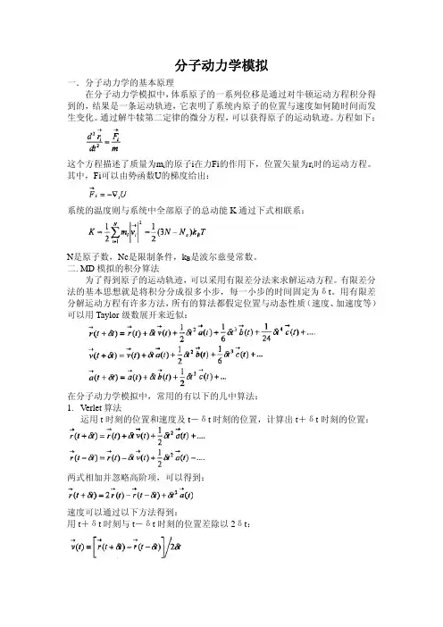
分子动力学模拟一．分子动力学的基本原理在分子动力学模拟中，体系原子的一系列位移是通过对牛顿运动方程积分得到的，结果是一条运动轨迹，它表明了系统内原子的位置与速度如何随时间而发生变化。

通过解牛犊第二定律的微分方程，可以获得原子的运动轨迹。

方程如下：这个方程描述了质量为m i的原子i在力Fi的作用下，位置矢量为r i时的运动方程。

其中，Fi可以由势函数U的梯度给出：系统的温度则与系统中全部原子的总动能K通过下式相联系：N是原子数，Nc是限制条件，k B是波尔兹曼常数。

二. MD模拟的积分算法为了得到原子的运动轨迹，可以采用有限差分法来求解运动方程。

有限差分法的基本思想就是将积分分成很多小步，每一小步的时间固定为δt。

用有限差分解运动方程有许多方法，所有的算法都假定位置与动态性质（速度、加速度等）可以用Taylor级数展开来近似：在分子动力学模拟中，常用的有以下的几中算法：1. Verlet算法运用t时刻的位置和速度及t－δt时刻的位置，计算出t＋δt时刻的位置：两式相加并忽略高阶项，可以得到：速度可以通过以下方法得到：用t＋δt时刻与t－δt时刻的位置差除以2δt：同理，半时间步t+δt时刻的速度也可以算：Verlet算法执行简单明了，存储要求适度，但缺点是位置r(t＋δt)要通过小项与非常大的两项2r(t)与r(t－δt)的差相加得到，容易造成精度损失。

另外，其方程式中没有显示速度项，在没有得到下一步的位置前速度项难以得到。

它不是一个自启动算法：新位置必须由t时刻与前一时刻t－δt的位置得到。

在t＝0时刻，只有一组位置，所以必须通过其它方法得到t－δt的位置。

一般用Taylor级数：2. Velocity－Verlet算法3. Leap-frog算法为了执行Leap-frog算法，必须首先由t-0.5δt时刻的速度与t时刻的加速度计算出速度v(t+δt)，然后由方程计算出位置r(t+δt)。

T时刻的速度可以由：得到。

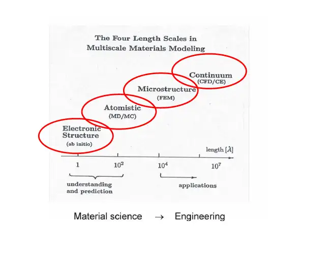
分⼦动⼒学与原⼦多体势解析⼀．分⼦动⼒学简介随着纳⽶科技的到来，许多新的学科产⽣了，例如纳⽶电⼦学、纳⽶⽣物学、纳⽶材料学、纳⽶机械学等。

⼈们的注意⼒逐渐从宏观物体转向⼩尺度及相应的器件，其中微机械系统(mieromachine)或称微型机电系统(mieroe⼀eetro⼀meeh耐ealsystem，MEMs)尤其取得了成功，并正被拓展应⽤于各种⼯业过程。

由图1可知，分⼦动⼒学正是处于nm尺度下的研究⽅法。

图1.不同模拟⽅法所对应的空间和时间尺度1957年Alder和Wainwright[1]开创了分⼦动⼒学(Moleeularnynamies，MD)⽅法，之后经过多位科学家的努⼒，拓展了分⼦动⼒学⽅法的理论、技术及应⽤领域，尤其是在20世纪80年代由Andersen等[2]先后完成的恒温、定压分⼦动⼒学⽅法，标志着分⼦动⼒学⽅法的科研应⽤进⼊了⼀个新阶段。

分⼦动⼒学⽅法是研究纳⽶尺度物理现象的重要⼿段。

随着越来越多的材料原⼦间作⽤势函数被精确描述并经过实验验证、计算机硬件⽔平的快速更新以及⾼效率新算法的提出，分⼦动⼒学模拟被⼴泛应⽤于纳⽶尺度⼒学⾏为和纳⽶材料⼒学性能的研究。

在纳⽶尺度下，材料由离散的原⼦排列⽽成，由于⽐表⾯积⼤、表⾯效应明显，材料的⼒学性能和⼒学⾏为将与宏观材料迥异。

基于连续性假设的宏观连续介质理论在研究材料的损伤演化、失效过程时，往往在时间和空间上将原⼦尺度的缺陷进⾏平均化处理，但这种处理仅适⽤于⼤量缺陷分布在材料中计算区域的情形，⽽对许多细微观材料和⼒学实验观测到的现象都⽆法解释，如疲劳与蠕变过程中的位错模式、塑性变形的不均匀性、脆性断裂的统计本质、尺⼨效应等。

因此，连续介质理论显然难以准确求解纳⽶尺度的⼒学问题。

同时，如果直接从第⼀原理出发进⾏计算，除了类氢原⼦以外其他材料的薛定愕⽅程求解难度都太⼤，⽽且局域密度泛函近似理论并不是总能满⾜实际问题的需要。

另⼀⽅⾯，材料本⾝在空间、时间和能量等⽅⾯存在藕合和脱祸现象[3,4]，直接从头开始的量⼦⼒学计算难以很好地应⽤到⼏百个原⼦以下的计算规模中，⽆法达到⼀般纳⽶材料和器件的模拟要求。

分子动力学分子动力学方法是一种计算机模拟实验方法，是研究凝聚态系统的有力工具。

该技术不仅可以得到原子的运动轨迹，还可以观察到原子运动过程中各种微观细节。

它是对理论计算和实验的有力补充。

分子动力学总是假定原子的运动服从某种确定的描述，这种描叙可以牛顿方程、拉格朗日方程或哈密顿方程所确定的描述，也就是说原子的运动和确定的轨迹联系在一起。

在忽略核子的量子效应和Born-Oppenheimer绝热近似下，分子动力学的这一种假设是可行的[1]。

所谓绝热近似也就是要求在分子动力学过程中的每一瞬间电子都处于原子结构的基态。

要进行分子动力学模拟就必须知道原子间的相互作用势。

在分子动力学模拟中，我们一般采用经验势来代替原子间的相互作用势，如Lennard-Jones势、Mores势、EAM原子嵌入势、F-S多体势。

然而采用经验势必然丢失了局域电子结构之间存在的强相关作用信息，即不能得到原子动力学过程中的电子性质[1]。

事实上，分子动力学就是模拟原子系统的趋衡过程。

实际上，分子动力学方法就是确定某一描述与初始条件、边值关系的数值解。

我们假定系统经过M步长之后达到稳定，而这一稳定状态正是我们所求的。

１、分子动力学的算法分析首先，我们假定我们研究的系统服从 Newton 方程所确定的描述，即：)(1)(..t F mt r =（1） 式中r(t)表征原子在t 时刻的位置矢量F(t)表征原子在t 时刻所受到的力，它与所有原子的位置矢有关m 表征原子的质量。

如果我们给定初始条件，即方程（１）的定解条件r(0)和v(0)，那么方程（１）的解就可以确定。

６０年代中期发展了大量的分子动力学算法，如两步差分算法[2]、预测-校正算法[3]、中心差分算法[4]、蛙跳算法[5]等等。

为了方便导出它们，我们以Euler 一步法[6]来讨论之。

我们令)()(..t r t v =（表征粒子的速度），则有：)()()(1)()(....t v t r t F m t r t v === （２）记⎥⎥⎥⎦⎤⎢⎢⎢⎣⎡=⎥⎦⎤⎢⎣⎡=)()(1)()()()(.t v t F m t f t r t v t w （３）则有)()(.t f t w = ？？？？？？ （４） 欧拉一步法就是用向前差商来替代一阶导数，即：)()()1(.t w hk w k w =-+，其中h 是时间步长，将之代入（４）则有：)()()1(t hf k w k w =-+ （５）即：⎥⎥⎦⎤⎢⎢⎣⎡=⎥⎦⎤⎢⎣⎡-+-+)()(1)()1()()1(k v k F m h k r k r k v k v )()()1()(1)()1(k hv k r k r k F mhk v k v +=++=+ （６） 对于（６）式,因为给定了r(0)和v(0),故r(k+1) 和v(k+1)可以确定。

分子动力学原理、算法简介与Gromacs的使用与G的使用部分内容选自超算中心2012年Gromacs培训教材中国科学院超级计算中心杨科大计算化学虚拟实验室（VLCC）计算化学虚拟实验室（VLCC）•高性能计算化学应用的新型虚拟科研组织•由网络中心和大连化物所于2004年发起成立•联合国内外知名计算化学科学家的平台•高性能计算化学与e‐Science应用研究•高性能计算化学应用促进研发SCChem系统、ICT‐HPCC国际会议、用户培训应用技术支持VLCC能为您的工作提供哪些帮助？1.提供正版计算化学软件1提供版计算化学软件2计算化学高性能计算的解决方案2.计算化学高性能计算的解决方案最近的工作：蛋白质折叠的新型高精度模拟软件的开发和移植最近的工作蛋白质折叠的新型高精度模拟软件的开发和移植AMNW在天河‐2节点上实现近30万核的并行执行，并行效率超过30%包含106个氨基酸的蛋白质体系，3392个子任务在142秒内实现5ps的蛋白质折叠计算模拟53计算程序的GPU/MIC并行移植3.计算程序的GPU/MIC并行移植最近的工作：1.耗散粒子动力学程序的GPU移植1耗散粒子动力学程序的GPU移植开发了新的大规模计算算法实现了相比于单CPU核约50倍的加速2.计算化学软件的MIC上编译实现2计算化学软件的MIC上编译实现NWchemAmber大家有计算化学方面的软件，硬件或合作问题，请联系我们：E‐mail: vlcc@微博：主要内容一：分子动力学模拟原理二：分子动力学模拟算法二分子动力学模拟算法三：Gromacs使用初步一：分子动力学模拟原理1.1 分子动力学模拟及其应用12分子动力学基本方程1.2 分子动力学基本方程1.3 分子力场1.3分子力场1.4 分子模拟的一般流程1.1分子动力学模拟及其应用Why MD simulations?•Model phenomena that cannot be observed experimentally •Access to thermodynamics quantities (free energies, binding energies,…)•Simulators and experimentalists can have a synergistic relationship, leading to new insights into materialsproperties•…First molecular dynamics simulation(1957/59)Hard disks and spheres⎧>dr 0(calculation of collision times)⎩⎨≤∞=dr r u ij )(IBM-704:solid phase liquid phaseliquid-vapour-phaseN=32: 7000 collisions / h Production run ~20000steps N=32 → 6.5x105coll. → 4 daysN=500: 500 collisions / hProduction run ~20000 stepsN=500 →107coll. → 2.3 years今天的分子动力学模拟生命科学纳米材料凝聚态物理如：水结晶，相分离（如：蛋白质折叠）如：分子马达药物设计2013年诺贝尔化学奖年诺贝尔化学奖将实验带入信息时代Martin KarplusArieh WarshelMichael Levitt复杂化学体系多尺度模型的发展算模结将实带信代量化计算与分子模拟的结合*所有图片来源于10m10mScaleLength Scale15Newton’s equations of motion)体系内粒子之间的相互作用能) (very important)1.3分子力场1.Bonded : covalent bond-stretching, angle-bending, and1.3 分子力场dihedrals. These are computed on the basis of fixed lists.2.Non-bonded : Lennard-Jones or Buckingham, and Coulomb or modified Coulomb. The nonbondedinteractions are computed on the basis of a neighbor list (a list of non-bonded atoms within a certain radius), in which exclusions are already removed.3.Restraints : position restraints, angle restraints, distance restraints, orientation restraints and dihedral restraints, all 17based on fixed lists.181.3.1 Bonded Interactionsbondalong rotate bend bond stretch bond bonded U U U U −−−−++=g Torsion anglesAre 4-body Non-bondedypairAngles A 3b d BondsA 2b d Are 3-body Are 2-body19Bonded Interactions: Bond StretchingHarmonic potential bHarmonic potentialFourth power potential p p Morse potential bond stretching for reasons of computational efficiency overstretching leads to infinitely low energies The for reasons of computational efficiency.overstretching leads to infinitely low energies. The integration time step is therefore limited to 1 fs .21t t h =−K b = Force Constant =Ideal Bond Length()2b o n d stretch b o p a irsU K b b −∑20b o = Ideal Bond LengthBonded Interactions:dihedral angleThe angle between planes (i,j,k) and (j,k,l)Figure 4.8: Principle of improper dihedral angles. Out of plane bending for rings (left),substituents of rings (middle), out of tetrahedral (right).Improper dihedralsFi 49I dih d l i lNote that in the input in topology files, angles are given indegrees and force constants in kJ/mol/rad 2.21Figure 4.9: Improper dihedral potential.1.3.2The Lennard-Jones interaction1264ij ij σσε=−(45)22(()())ij ij r r (4.5)occupies a certain amount of space. If atoms are brought too close together, there isrepulsion), and this may affect the molecule's preferred shapeNon‐Bonded Interactions: van der Waals Buckingham potentialFigure 4.2: The Buckingham interaction.23The25二：分子动力学模拟算法2.1 非键接力的计算211短程相互作用计算2.1.1 短程相互作用计算2.1.2 静电相互作用2.2 积分、压力和温度控制2.3 能量最小化23能量最小化2.1.1短程相互作用计算Short-range force calculation→ save CPU time by using neighbor lists neighbor list:neighbor list:27cell list:most efficient is a combination ofVerlet and cell list. (8 neighbor cellsfor 2D 26neighbor cells for 3D )update when a particle hasmade a displacementfor 2D, 26 neighbor cells for 3D.)made a displacement > (r skin -r cut )/2大规模并行策略：Domain decomposition•Partition space, instead of atoms, over nodes•Good for load balancing (uniform system, what about non-uniform system?)•Bad for communication bandwidth•Each node ‘imports’ coordinate and exports forces from neighbors within a sphere with radius=cutoff.2.1.2静电相互作用周期性边界条件下静电相互作用的计算2.1.2 静电相互作用q q 11N N i jU =11042|+|=x y z coul n n n i j ij x y z n n n πε==++∑∑∑∑∑r n n x y z算法复杂度：N 2NonbondedInteractions: EwaldSum Ewald Sum近程相互作用远程相互作用FFT is a finite and discrete Fourier transformation th s point charges ith 关联相互作用Standard Ewald implementation scales like N 2Most costly part: Fourier transformation transformation, thus point charges with continuous coordiates have to be replacedby a grid based charge density (step 1).Process can be speeded up by a method called “Fast Fourier Transformation” (FFT)PME的并行策略：2.2 Numeric Integration MethodVerlet’s Numeric Integration MethodTaylor expansion:Verlet’s Method*Verlet., L. Computer experiments on classical fluids. i. thermodynamical properties of lennard-jones molecules. Phys. Rev.159:98–103, 1934Leap‐frogNumericIntegration MethodThe MD program utilizes the so-called leap-frog algorithm* for the integration of the equations of motion. The leap-frog algorithm uses positions r at time t and velocities at time /2;it updates positions and velocities using the forces )determined v at time t -Δt /2 ; it updates positions and velocities using the forces F (t ) determined by the positions at time t :Figure 3.6: The Leap-Frog integration method. The algorithm is called Leap-Frog because rIt is equivalent to the Verlet algorithm. The algorithm is of third order in r and is time-reversible.and v are leaping like frogs over each others’ back.time reversible.Berendsen temperature couplingThe Berendsen algorithm mimicsthe number of degrees of freedom and d W a Wiener process. There are no additionalThis thermostat produces a correct canonical ensemble and still has thethermostat: first order decay of temperature deviations and no oscillations.When an NVT ensemble is used, the conserved energy quantity is written to the energy and log file.Berendsen et al. Molecular dynamics with coupling to an external bath. J. Chem. Phys. 81:3684 (1984)Nose-Hoover (chain) temperature couplingThe Berendsentarget temperature,τTkinetic energy between the system and the reservoir instead. It is directly related to Q and T0via(3.29)This provides a much more intuitive way of selecting the Nose-Hoover coupling strength (similar to theis independent of system size and reference temperature.2.2 Temperature control schemesIt is however important to keep the difference between the weak coupling scheme and the Nose-Hoover algorithm in mind:¾Using weak coupling you get a strongly damped exponential relaxation,while the Nose-Hoover approach produces an oscillatory relaxation.¾The actual time it takes to relax with Nose-Hoover coupling is several times larger than the period of the oscillations that you select.¾These oscillations (in contrast to exponential relaxation) also means that the time constant normally should be 4–5 times larger than the relaxation time used with weak coupling,but your mileage may vary.li b ilGroup temperature couplingIn GROMACS temperature coupling can be performed on groups of atoms, typically a protein andIn GROMACS temperature coupling can be performed on groups of atoms typically a protein and solvent. The reason such algorithmes were introduced is that energy exchange between different components is not perfect, due to different effects including cutoffs etc. If now the whole system is coupled to one heat bath, water (which experiences the largest cutoff noise) will tend to heat up and the protein will cool down.Typically 100 K differences can be obtained. With the use of proper electrostatic methods (PME) these difference are much smaller but still not negligable. The parameters for temperature coupling in groups are given in the mdp file. One special case should be mentioned: it is possible to T-couple only part of the system(or nothing at all obviously)This is done by specifying is possible to T couple only part of the system (or nothing at all obviously). This is done by specifying zero for the time constant τT for the group of interest.2.2 Simulating at constant P In the same spirit as the temperature coupling, the system can also be coupled to a ‘pressure bath’. GROMACS supports both theBerendsen algorithm * that scales coordinates and box vectors every step, and the extended ensemble Parrinello-Rahman approach . Both of these can be combined with any of the temperature coupling methods above.Berendsen pressure couplingTh B d l ith l th di t d b t t ith t i The Berendsen algorithm rescales the coordinates and box vectors every step with a matrix ,which has the effect of a first-order kinetic relaxation of the pressure towards a given reference pressure P 0:The scaling matrix is given byHere is the isothermal compressibility of the system. In most cases this will be a βp y ydiagonal matrix, with equal elements on the diagonal, the value of which is generally not known.For water at 1atm and 300K:=46-10-1=46-5-1Berendsen et al. Molecular dynamics with coupling to an external bath. J. Chem. Phys. 81:3684 (1984)For water at 1 atm and 300 K: β= 4.6×1010Pa 1= 4.6×105Bar 12.2 Simulating at constant P Parrinello Rahman pressure coupling Parrinello-Rahman pressure couplingIn cases where the fluctuations in pressure or volume are important per se (e.g. to calculate thermodynamic properties) it might at least theoretically be a problem that the exact bl i ll d fi d f h k li hensemble is not well-defined for the weak coupling scheme.For this reason, GROMACS also supports constant-pressure simulations using theParrinello-Rahman approach*, which is similar to the Nose-Hoover temperature coupling. With th P i ll R h b t t th b t t d b th t i b With the Parrinello-Rahman barostat, the box vectors as represented by the matrix b obey the matrix equation of motion.The volume of the box is denoted V , and W is a matrix parameter that determines thestrength of the coupling. The matrices P and P are the current and reference pressures, g p g ref p ,respectively.The (inverse) mass parameter matrix W -1determines the strength of the coupling, and howthe box can be deformed the box can be deformed.Y l h id h i i h l ibili i d h40You only have to provide the approximate isothermal compressibilities βand the pressure time constant τp in the input file (L is the largest box matrix element)2.2 Simulating at constant PThe equations of motion for the particles are also changed, just as for the Nose-Hoover coupling. In most cases you would combine the Parrinello-Rahman barostat with the Nose Hoover thermostat, but to keep it simple we only show the Parrinello Rahman Nose-Hoover thermostat,but to keep it simple we only show the Parrinello-Rahman modification here:Just as for the Nose-Hoover thermostat, you should realize that the Parrinello-Rahman time Just as for the Nose-Hoover thermostat you should realize that the Parrinello-Rahman time constant is not equivalent to the relaxation time used in the Berendsen pressure coupling algorithm.In most cases you will need to use a 4–5 times larger time constant with Parrinello-Rahman I t ill d t45ti l ti t t ith P i ll R h coupling. If your pressure is very far from equilibrium, the Parrinello-Rahman coupling may result in very large box oscillations that could even crash your run. In that case you would have to increase the time constant, or (better) use the weak coupling scheme to reach would have to increase the time constant or(better)use the weak coupling scheme to reach the target pressure, and then switch to Parrinello-Rahman coupling once the system is in equilibrium.412.3 能量最小化EnergyMolecular dynamicsuses thermal energyto explore the energysurfacefState AState BEnergy minimizationEnergy minimizationstops at local minimaSteepest descent (SD,最陡下降算法):The simplest iteration scheme consists of following the “steepest descent” direction:)(1k k k x f x x ∇−=+α(αsets the minimum along the line definedby the gradient)Usually, SD methods leads to improvement quickly, but then exhibit slow progress toward a solution.Th l d d f i iti l i i i ti it ti by the gradient)They are commonly recommended for initial minimization iterations,when the starting function and gradient-norm values are very large.43Illustration of the steepest (gradient) descent method.DisadvantagesAs per the examples, the disadvantagesof this method are as follows:•it is relatively slow close to the minimum;•the linear search may cause problems;integrator = steep emtol = 100.0 ; in kJ mol^-1 nm^-1emstep = 0.002 ; in nm44•it might 'zigzag' down valleys.Conjugate gradients (CG):In each step of conjugate gradient methods, a search vector p defined by a recursive formula:[])()(1k k x f x f ∇−∇•+45])()(1k k x f x f ∇−∇+Conjugate gradients (CG)：A comparison of the convergence of gradientdescent(in green)and conjugate gradient(in red)In general,steepest descents willbring you close to the nearest localminimum very quickly,whileconjugate gradients brings you veryclose to the local minimum,butperforms worse far away from theminimum.46Newton’s methodL-BFGS is particularly well suited for optimization problems with a large number of dimensions.In practice this seems to converge faster than Conjugate Gradients, but due to the correction steps necessary it is三：Gromacs使用初步3.1 Gromacs的安装32输入文件准备3.2 输入文件准备3.3 作业运行、提交3.3作业运行、提交3.4 练习3.1 Gromacs的安装Install Gromacs4.5.5Check compiler and mpi environment which ifortwhich iccwhich mpiccwhich mpicc...INSTALLATIONInstall Gromacs4.5.5 –Serial version source /opt/intel/Compiler/11.1/073/bin/ifortvars.sh intel64source /opt/intel/Compiler/11.1/073/bin/iccvars.sh intel64export MKL_PATH=/opt/intel/Compiler/11.1/073/mklexport CC=icc./configure --prefix=/opt/gromacs-4.5.5makemake installmake links (optional)k li k(ti l)Note: default is to use “--enable-shared”。

分子动力学中文
分子动力学是一门结合物理、数学和化学的综合技术，是一套分子模拟方法。

该方法主要依靠牛顿力学来模拟分子体系的运动，以在由分子体系的不同状态构成的系综中抽取样本，从而计算体系的构型积分，并以构型积分的结果为基础进一步计算体系的热力学量和其他宏观性质。

分子动力学是一种计算机辅助模拟工具，用于描述物质或分子中的原子级运动过程。

其基本过程为：1. 设置研究对象组成原子的初始位置和速度；2. 计算每个原子受到的合力，并基于牛顿第二定律计算原子的加速度；3. 计算原子下一时刻的速度；4. 计算原子下一时刻的位置；5. 循环2-4的过程，得到一系列时刻原子的位置和速度；6. 基于位置和速度信息得到描述对象性质和行为的物理量。

分子动力学在多个领域中都有广泛的应用，如固态、液态、软物质、粗粒化物质等领域。

其中，LAMMPS是一款开源的分子动力学模拟软件，可以支持十亿级原子规模的计算，在计算能力和效率方面表现出色。