stata软件meta分析操作详细攻略报告

meta分析步骤详解，以及常见问题解析Meta分析的完整步骤，根据个⼈的体会，结合各位友⼈的经验总结⽽成，meta的精髓就是对⽂献的⼆次加⼯和定量合成，所以这个总结也算是对⼤家经验的meta分析吧。

▽⼀、选题和⽴题1形成需要解决的临床问题系统评价可以解决下列临床问题:1. 病因学和危险因素研究;2. 治疗⼿段的有效性研究;3. 诊断⽅法评价;4. 预后估计;5. 病⼈费⽤和效益分析等。

进⾏系统评价的最初阶段就应对要解决的问题进⾏精确描述,包括⼈群类型(疾病确切分型、分期)、治疗⼿段或暴露因素的种类、预期结果等,合理选择进⾏评价的指标。

2指标的选择直接影响⽂献检索的准确性和敏感性，关系到制定检索策略。

3制定纳⼊排除标准。

⼆、⽂献检索1检索策略的制定这是关键，要求查全和查准。

推荐Mesh联合free word检索。

2⽂献检索，获取摘要和全⽂国内的有维普全⽂VIP，CNKI，万⽅数据库，外⽂的有medline ,SD，OVID等。

3⽂献管理强烈推荐使⽤endnote，procite，noteexpress等⽂献管理软件进⾏检索和管理⽂献。

查找⽂献全⽂的途径在这⾥，讲⼀下找⽂献的过程，以请后来的朋们参考（不包括⽹上有电⼦全⽂的）：1. 查找免费全⽂（1）在pubmed center中看有⽆免费全⽂。

有的时候虽然没有显⽰free full text，但是点击进去看全⽂链接也有提供免费全⽂的。

我就碰到⼏次。

（2）在google中搜⼀下。

少数情况下，NCBI没有提供全⽂的，google有可能会找到，使⽤“学术搜索”。

本⼈虽然没能在google中找到⼀篇所需的⽂献，但发现了⼀篇⾮常重要的综述，⾥⾯包含了所有我需要的⽂献（当然不是数据），但起码提供了⼀个信息，所需要的⽂献也就这么多了，因为⽼外的综述也只包含了这么多的内容。

这样，到底找多少⽂献，找什么⽂献，⼼⾥就更有底了。

（3）免费医学全⽂杂志⽹站。

提供很过超过收费期的免费全⽂。

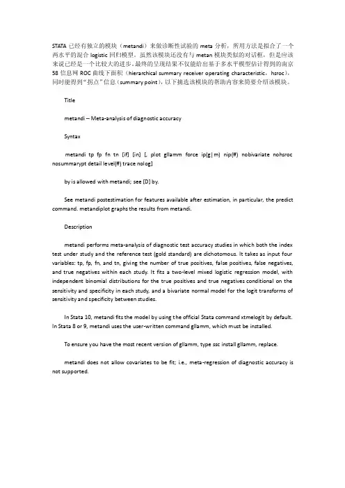
STATA已经有独立的模块（metandi）来做诊断性试验的meta分析，所用方法是拟合了一个两水平的混合logistic回归模型。

虽然该模块还没有与metan模块类似的对话框，但是应该来说已经是一个比较大的进步。

最终的呈现结果不仅能给出基于多水平模型估计得到的南京58信息网ROC曲线下面积（hierarchical summary receiver operating characteristic，hsroc），同时能得到“拐点”信息（summary point），以下摘选该模块的帮助内容来简要介绍该模块。

Titlemetandi -- Meta-analysis of diagnostic accuracySyntaxmetandi tp fp fn tn [if] [in] [, plot gllamm force ip(g|m) nip(#) nobivariate nohsroc nosummarypt detail level(#) trace nolog]by is allowed with metandi; see [D] by.See metandi postestimation for features available after estimation, in particular, the predict command. metandiplot graphs the results from metandi.Descriptionmetandi performs meta-analysis of diagnostic test accuracy studies in which both the index test under study and the reference test (gold standard) are dichotomous. It takes as input four variables: tp, fp, fn, and tn, giving the number of true positives, false positives, false negatives, and true negatives within each study. It fits a two-level mixed logistic regression model, with independent binomial distributions for the true positives and true negatives conditional on the sensitivity and specificity in each study, and a bivariate normal model for the logit transforms of sensitivity and specificity between studies.In Stata 10, metandi fits the model by using the official Stata command xtmelogit by default. In Stata 8 or 9, metandi uses the user-written command gllamm, which must be installed.To ensure you have the most recent version of gllamm, type ssc install gllamm, replace.metandi does not allow covariates to be fit; i.e., meta-regression of diagnostic accuracy is not supported.。

stata meta回归结果详细解读Meta回归是一种统计方法，用于整合多个独立研究的结果，以得出一个总体效应估计。

在Stata中进行Meta回归分析后，我们主要通过以下几种统计量和图形进行结果的解读：1. 森林图：这是一种用于展示多个研究的效应量、置信区间和权重的图形。

横线上的点代表单个研究的效应量，横线长度代表该效应量的95%置信区间范围，横线上的方块大小代表该研究的权重，即该项研究对Meta分析的贡献度。

图中的菱形则代表合并后的结果；图中的垂直实线是无效线，用于判定结果差异有无统计学意义，若单个研究或合并效应量的95%置信区间与该直线相交，则代表两组的差异没有统计学意义。

2. Q统计量和I2统计量：Q统计量是服从自由度为K-1的卡方分布，本质是卡方检验，属于异质性定性分析的方法。

一般认为当P<0.1时，表明各研究间存在异质性。

3. 气泡图：这是另一种用于展示Meta回归结果的图形，例如以年龄为协变量的气泡图。

在进行Meta回归分析时，还需要注意以下几点：- 异质性检验：通过Q统计量和I2统计量进行异质性检验，以判断各研究间是否存在显著差异。

- 亚组分析和敏感性分析：这些分析可以帮助我们更深入地了解Meta回归结果的稳定性和可靠性。

我们还可以通过查看回归系数和其95%置信区间来评估每个协变量对因变量的影响。

如果回归系数的95%置信区间不包含零，那么我们可以得出结论说该协变量对因变量有显著影响。

我们还需要注意可能存在的一些偏倚问题，如出版偏倚、选择偏倚等。

这些问题可能会影响到Meta回归结果的准确性和可靠性。

因此，在进行Meta回归分析时，我们需要尽可能地选择那些经过同行评审的研究，并考虑使用一些方法来修正可能存在的偏倚问题。

Meta回归是一种强大的统计工具，可以帮助我们从大量的独立研究中提取出有用的信息。

然而，正确地解读Meta回归结果需要一定的专业知识和经验。

如果你不确定如何解读你的结果，或者你对结果有任何疑问，你应该寻求专业的统计咨询。

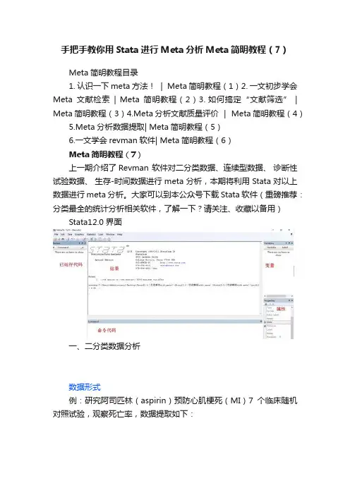
手把手教你用Stata进行Meta分析Meta简明教程（7）Meta简明教程目录1. 认识一下meta方法！ | Meta简明教程（1）2. 一文初步学会Meta文献检索| Meta简明教程（2）3. 如何搞定“文献筛选” | Meta简明教程（3）4.Meta分析文献质量评价 | Meta简明教程（4）5.Meta分析数据提取| Meta简明教程（5）6.一文学会revman软件| Meta简明教程（6）Meta简明教程（7）上一期介绍了Revman 软件对二分类数据、连续型数据、诊断性试验数据、生存-时间数据进行meta分析，本期将利用Stata对以上数据进行meta分析。

大家可以到本公众号下载Stata软件（重磅推荐：分类最全的统计分析相关软件，了解一下？请关注、收藏以备用）Stata12.0 界面一、二分类数据分析数据形式例：研究阿司匹林（aspirin）预防心肌梗死（MI）7个临床随机对照试验，观察死亡率，数据提取如下：操作步骤1.构建数据1)启动Stata 12.0 软件后，可以直接点击工具栏中DataEditor (edit)按钮。

也可在在菜单栏中点击Data→Data Editor→ DataEditor (edit)，出现以下界面。

2）点击变量名位置，依次输入研究名称（research），阿司匹林组死亡数(a)，阿司匹林组存活数(b)，安慰剂组死亡数(c)，安慰剂组存活数(d)3）录入数据：在变量值区域输入数据2. 数据分析1）导入meta模块：在Command窗口中进行编程，首先需要在Stata中安装meta 模块:在Command窗口输入“ssc install metan”，选中点回车。

结果窗口中出现下面的结果，说明已经安装了meta模块。

2）输入meta分析代码：在Command窗口输入“Command窗口输入“metan a b c d, or fixed”,点回车，完成结果分析。

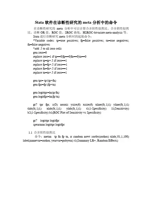
Stata软件在诊断性研究的meta分析中的命令在诊断性研究的meta分析中可以计算合并阳性似然比、合并阴性似然比、诊断OR值、ROC值、SROC曲线、HSROC-bivariate meta-analysis等。

Stata进行诊断研究meta分析时的起始命令：*Variable codes: tp=true positives; fp=false positives; tn=true negatives;fn=false negatives*add .5 to all zero cellsgen zero=0replace zero=1 if tp==0|fp==0|fn==0|tn==0replace tp=tp+.5 if zero==1replace fp=fp+.5 if zero==1replace fn=fn+.5 if zero==1replace tn=tn+.5 if zero==1gen tpr= tp/(tp+fn)gen fpr=fp/(fp+tn)gen logittpr=ln(tp/fn)gen logitfpr=ln(fp/tn)gr7 tpr fpr, s(O) noaxis ysize(6) xsize(6) xline(0(.1)1) yline(0(.1)1) tlab(0(.1)1) xlab(0(.1)1) ylab(0(.1)1) t1(1-Specificity) l1(Sensitivity) b2(1-Specificity) b1(ROC Plot of Sensitivity vs Specificity)gr7 logittpr logitfprspearman logittpr logitfpr1.1 合并阳性似然比命令：metan tp fn fp tn, rr random nowt sortby(author) xlab(.01,1,100) label(namevar=author, yearvar=pubyear) t1(Summary LR+, Random Effects)2.2 合并阴性似然比命令：metan fn tp tn fp, rr random nowt sortby(author) xlab(.01,1,100) label(namevar=author, yearvar=pubyear) t1(Summary LR-, Random Effects)2.3 合并诊断OR值命令：metan tp fn fp tn, or random nowt sortby(author) xlab(.01,1,100) label(namevar=author, yearvar=pubyear) t1(Summary Diagnostic Odds Ratio, Random Effects)2.4 ROC值命令：gr7 tpr fpr, s(O) noaxis ysize(6) xsize(6) xline(0(.1)1) yline(0(.1)1) tlab(0(.1)1) xlab(0(.1)1) ylab(0(.1)1) t1(1-Specificity) l1(Sensitivity) b2(1-Specificity) b1(ROC Plot of Sensitivity vs Specificity)2.5 SROC曲线命令：gen sum= logittpr+ logitfprgen diff= logittpr- logitfprregress diff sumpredict yhatgr7 diff yhat sum, ylab(3,4,5,6,7,8) xlab(-4,-3,-2,-1,0,1,2) c(.l) s(oi)gen tse=1/(1+(1/(exp(_cons/1-_b)*(fpr/spec)^1+_b/1-_b)))(constant and b are derived from the above regression model)*plot SROC curve (generic)gr7 se tse fpr, ysize(6) xsize(6) noaxis xline(0(.1)1) yline(0(.1)1) tlab(0(.1)1) xlab(0(.1)1)ylab(0(.1)1) s(Oi) c(.s) l1(Sensitivity) b2(1-Specificity) ti(Summary ROC Curve) key1(" ")key2(" ")2.6 HSROC-bivariate meta-analysis命令：metandi tp fp fn tn, plot （基于SROC命令）2.7 发表偏倚命令：gen or=(tp*tn)/(fp*fn)gen lnor=ln(or)gen selnor=(1/tp)+(1/fp)+(1/fn)+(1/tn)*Begg and Egger test for publication bias with Begg's funnel plot: metabias lnor selnor, graph(begg)*Begg and Egger tests for subgroups (eg. Covariate=1)metabias lnor selnor if covariate==1, graph(begg)。

Meta回归stata结果解读在统计学中，meta回归分析是一种用于结合多个独立研究结果的方法，以产生一个综合的估计值。

这种方法可以帮助研究者更准确地评估一个特定效应的大小和方向，并且可以提供对这个效应的整体理解。

在本文中，我们将介绍meta回归分析的基本概念，并对使用Stata软件进行meta回归分析的结果进行解读。

1. 概念在研究领域，通常会有多个独立的研究对同一个问题或效应进行研究，并且产生了不同的估计值。

meta回归分析的主要目的就是将这些独立研究的结果进行合并，得出综合的效应估计。

这样做的好处是可以增加研究结果的统计功效，并且可以提供更准确的估计。

2. Stata软件进行meta回归分析利用Stata软件进行meta回归分析可以帮助研究者更方便地进行数据处理和结果解读。

我们需要将已有的研究结果数据导入Stata软件中，然后使用meta命令进行meta回归分析。

在得到结果后，我们可以对各个参数进行解读，并得出综合的效应值和其置信区间。

3. 结果解读在meta回归分析的结果中，我们通常会看到各个研究的效应值、加权效应值、置信区间等参数。

在解读这些结果时，我们需要重点关注综合的效应值和其置信区间。

如果置信区间包含0，说明综合效应值可能不显著；而如果置信区间不包含0，说明综合效应值可能是显著的。

我们还需要关注异质性检验的结果，以确定研究结果是否存在显著的异质性。

4. 个人观点个人对meta回归分析的理解是，这种方法可以帮助研究者更全面地评估一个效应的大小和方向，尤其是当存在多个独立研究时。

利用Stata软件进行meta回归分析，可以更加方便地进行数据处理和结果解读，为研究者提供了一个强大的工具。

总结在本文中，我们介绍了meta回归分析的基本概念，并介绍了利用Stata软件进行meta回归分析的方法和结果解读。

通过对结果的解读，我们可以更全面地评估一个效应的大小和方向，从而得出对研究问题的更深入理解。

Both the output and the graph show that there is a clear effect of streptokinase in protecting against death following myocardial infarction. The meta-analysis is dominated by the large GISSI-12and ISIS-23trials which contribute 76·2% of the weight in this analysis. If required, the text showing the weights or treatment effects may be omitted from the graph (options nowt and nostats, respectively). The metan command will perform all the commonly used fixed effects (inverse variance method, Mantel–Haenszel method and Peto’s method) and random effects (DerSimonian and Laird) analyses. These methods are described in Chapter 15. Commands labbe to draw L’Abbé plots (see Chapters 8 and 10) and funnel to draw funnel plots (see Chapter 11) are also included. 352Note that meta performs both fixed and random effects analyses by default and the tabular output includes the weights from both analyses. It is clear that the smaller studies are given relatively more weight in the random effects analysis than with the fixed effect model. Because the meta command requires only the estimated treatment effect and its standard error, it will be particularly useful in meta-analyses of studies in which the treatment effect is not derived from the standard 2 ×2 table. Examples might include crossover trials, or survival trials, when the treatment effect might be measured by the hazard ratio derived from Cox regression. Example 2: intravenous magnesium in acute myocardial infarction The following table gives data from 16 randomised controlled trials of intravenous magnesium in the prevention of death following myocardial infarction. These trials are a well-known example where the results of a meta-analysis8were contradicted by a single large trial (ISIS-4)9–11(see also Chapters 3 and 11).355Dealing with zero cellsWhen one arm of a study contains no events – or, equally, all events – we have what is termed a “zero cell” in the 2 ×2 table. Zero cells create problems in the computation of ratio measures of treatment effect, and the standard error of either difference or ratio measures. For trial number 8 (Bertschart), there were no deaths in the intervention group, so that the estimated odds ratio is zero and the standard error cannot be estimated. A common way to deal with this problem is to add 0·5 to each cell of the 2 ×2 table for the trial. If there are no events in either the intervention or control arms of the trial, however, then any measure of effect summarised as a ratio is undefined, and unless the absolute (risk difference) scale is used instead, the trial has to be discarded from the meta-analysis.The metan command deals with the problem automatically, by adding 0·5 to all cells of the 2 ×2 table before analysis. For the commands which require summary statistics to be calculated (meta,metacum,metainf, metabias and metareg) it is necessary to do this, and to drop trials with no events or in which all subjects experienced events, before calculating the treatment effect and standard error.To drop trials with no events or all events:drop if dead1==0&dead0==0drop if dead1==tot1&dead0==tot0357By the late 1970s, there was clear evidence that streptokinase prevented death following myocardial infarction. However it was not used routinely until the late 1980s, when the results of the large GISSI-1 and ISIS-2 trials became known (see Chapter 1). The cumulative meta-analysis plot makes it clear that although these trials reduced the confidence interval for the summary estimate, they did not change the estimated degree of protection.Examining the influence of individual studiesThe influence of individual studies on the summary effect estimate may be displayed using the metainf command.15This command performs an influence analysis, in which the meta-analysis estimates are computed omitting one study at a time. The syntax for metainf is the same as that for the meta command. By default, fixed-effects analyses are displayed. Let’s perform this analysis for the magnesium data:metainf logor selogor, eform id (trialnam)361The label above the vertical axis indicates that the treatment effect estimate (here, log odds ratio) has been exponentiated. The meta-analysis is dominated by the ISIS-4 study, so omission of other studies makes little or no difference. If ISIS-4 is omitted then there appears to be a clear effect of magnesium in preventing death after myocardial infarction.Funnel plots and tests for funnel plot asymmetryThe metabias command16,17performs the tests for funnel-plot asymmetry proposed by Begg and Mazumdar18and by Egger et al.11(see Chapter 11). If the graph option is specified the command will produce either a plot of standardized effect against precision11(graph(egger)) or a funnel plot (graph(begg)). For the magnesium data there is clear evidence of funnel plot asymmetry if the ISIS-4 trial is included. It is of more interest to know if there was evidence of bias before the results of the ISIS-4 trial were known. Therefore in the following analysis we omit the ISIS-4 trial:metabias logor selogor if trial<16, graph(begg)Note: default data input format (theta, se_theta) assumed.if trialno < 16362The funnel plot appears asymmetric, and there is evidence of bias using the Egger (weighted regression) method (P for bias 0·007) but not using the Begg (rank correlation method). This is compatible with a greater statistical power of the regression test, as discussed in Chapter 11. The horizontal line in the funnel plot indicates the fixed-effects summary estimate (using363To use the metareg command, we need to derive the treatment effect estimate (in this case log risk ratio) and its standard error, for each study.generate logrr=log((cases1/tot1)/(cases0/tot0)) generate selogrr=sqrt((1/cases1)-(1/tot1)+(1/cases0)-(1/tot0))In their meta-analysis, Colditz et al. noted the strong evidence for heterogeneity between studies, and concluded that a random-effects meta-analysis was appropriate:meta logrr selogrr, eformMeta-analysis (exponential form)Pooled95% CI Asymptotic No. ofies MethodEst Lower Upper z_value p_value stud Fixed0.6500.6010.704-10.6250.00013 Random0.4900.3450.695-3.9950.000Test for heterogeneity: Q= 152.233 on 12 degrees of freedom (p= 0.000)Moment-based estimate of between studies variance = 0.309366。

用stata软件做单个样本率的meta分析
本实例采用的数据是本人的另一个贴子用的数据是这个贴子中我能用stata做患病率的meta分析了，大家交流交流啊 - 丁香园论坛中网友在别的文章中看到并上传的一个森林图：
这个森林图中的数据其实不太好，因为异质性太大，但数据简单，也就给大家摸拟一下。

重要的是知道怎样用stata软件做单样本率meta 分析就可以了。

在stata中要做meta分析，最重要的就是要知道两个变量，一个是ES也就是效应量，另一个是seES,也就效应量，所有关于率的meta,做meta的关键也就是如何去寻找这两个东东了,
我这里采用的就是直接用率做为ES,而ES的标准误其实也不难求出,大家可以看看孙振球教授《医学统计学》中的这个例子或许会有所启发:如下图
这个是基于正态近似法的公式,在样本量较,数据正态时使用,这算ES 的标准误也是如用的这个公式
下面开始具体操作:
1,输入数据,数据的格式是study,率，以及样本量
第二步：generate ser=sqrt(r*(1-r)/n)
3，用随机效应模型进行分析命令如下：metan r ser, random label(namevar=study)
继续
4，输入如下命令得到漏斗图:metafunnel r ser。

使用stata进行meta分析的详细具体过程和方法meta, stata最近使用stata 8进行meta分析，之前已经使用refman 5进行了初步处理，但是refman 的漏斗图只能粗略看是否对称，无法定量，据说stata可以进行发表性偏倚定量评价，所以自己摸索stata中的meta分析方法，在DXY中学习了不少战友的帖子（zhangdog战友），都感觉不是很系统，有的还有些问题。

结合自己的体会，写个详细的总结，希望对像我一样的初学者有所帮助，尤其对很多非统计学专业的人员有用，当然我也不是统计学专业的，问题再所难免，共同学习，还望战友指点。

1.stata的安装，建议下载8.0的版本，有战友反映9.0和10.0的版本好象有些问题，反正基本功能有了，meta分析的菜单在8.0以后版本都有了，所以不必追求最新的。

我是在上下载的。

baidu，google上都能找到。

2.原始数据的录入，这是应用stata进行分析的基础。

（1）命令窗口输入：Input no study event1 total1 event0 total0: |( g; m- [2 `; b3 `（分别表示纳入研究序号，名称，暴露组或处理组例数，总例数，对照组例数，对照组总例数，因为我是用refman中导出数据，这后4项可以直接输出），作用是产生变量。

然后可以逐行输入数据，以end命令结束，我建议初学者跳到下面的输入更简单。

* s# ?- w; d: B6 v$ L- j（2）点Data——Data editor（或ctrl＋7快捷键），可以直接录入数据，可以直接复制，粘贴数据。

输完后点击preserve保存退出Data editor 窗口。

6 z7 T5 M3 H5 ~%第一步（1）也可以省略，进入第二步后，先输入数据，然后双击自动产生的变量var1,var2....进行变量名称的修改，个人感觉这样快捷。

1 Deng SL 2004 31 114 8 100* Z4 U' m+ R$ i4 i8 V( P&2 Ding HF 2006 19 25 5 8^3 h2 l* t6 W9 ?" \$ _" o- S3 Fang ZL 2002 35 36 20 35+ C& ?* ^) Q3 y! l R, F' F14 Ito K 2006 36 40 31 40@5 ?* E& [!5 Kao JH 2003 81 127 4 35m/ y4 w2 R. y: h4 ~5 a6 Yuen MF 2004 60 66 101 1351 V3 [0 M& Y4 ~. B. x- a. B% l*完毕在命令窗输入list命令查看数据。

用stata软件做单个样本率的meta分析
本实例采用的数据是本人的另一个贴子用的数据是这个贴子中我能用stata做患病率的meta分析了，大家交流交流啊- 丁香园论坛中网友在别的文章中看到并上传的一个森林图：
这个森林图中的数据其实不太好，因为异质性太大，但数据简单，也就给大家摸拟一下。

重要的是知道怎样用stata软件做单样本率meta分析就可以了。

在stata中要做meta分析，最重要的就是要知道两个变量，一个是ES也就是效应量，另一个是seES,也就效应量，所有关于率的meta,做meta的关键也就是如何去寻找这两个东东了,
我这里采用的就是直接用率做为ES,而ES的标准误其实也不难求出,大家可以看看孙振球教授《医学统计学》中的这个例子或许会有所启发:如下图
这个是基于正态近似法的公式,在样本量较,数据正态时使用,这算ES的标准误也是如用的这个公式
下面开始具体操作:
1,输入数据,数据的格式是study,率，以及样本量
第二步：generate ser=sqrt(r*(1-r)/n)
3，用随机效应模型进行分析命令如下：metan r ser, random label(namevar=study)
继续
4，输入如下命令得到漏斗图:metafunnel r ser。

Stata教程：两组连续变量的Meta分析一、问题与数据Siristatidis等人拟探讨在辅助生殖技术中，使用促性腺激素释放激素激动剂的时间长短是否会对患者卵母细胞的数量产生影响。

试验组：卵巢刺激前至少2周开始使用；对照组：卵巢刺激开始时再使用。

研究者通过检索数据库，对最终纳入的文献，提取了如下信息：作者、发表年代、试验组样本量、试验组卵母细胞数量的均值、试验组卵母细胞数量的标准差、对照组样本量、对照组卵母细胞数量的均值、对照组卵母细胞数量的标准差。

最终纳入4篇研究，合计227名妇女。

各研究提取得到的数据如表1。

试问：在辅助生殖技术中，卵巢刺激前至少2周开始使用促性腺激素释放激素激动剂的患者，其卵母细胞的数量是否多于卵巢刺激开始时再使用的患者？表1. 文献信息提取表如果原始研究直接报告了结局变量的均值和标准差，则直接使用报告的值，如本例中试验组和对照组卵母细胞数量的均值和标准差。

如果原始研究未直接报告结局变量的均值和标准差，但报告了干预前、后结局变量的均值和标准差，则可以参照Cochrane Handbook 5.0.2中16.1.3.2提供的方法，计算干预前后结局变量变化的均值和标准差，即我们进行Meta分析所需要的均值和标准差：Mean E, change=Mean E, final - Mean E, baseline其中，Corr 取0.40或0.50。

举例说明：拟探讨胸腺五肽联合常规抗结核方案的复治菌阳肺结核患者，其CD3+的水平是否高于常规抗结核治疗的患者。

试验组：胸腺五肽联合常规抗结核方案；对照组：常规抗结核治疗。

(1) 打开数据录入窗口：Data →Data Editor →Data Editor (Edit)关于数据录入细节，可参考文章：Stata做Meta分析：以诊断试验准确性为例。