随机模拟(仿真)-simulation
- 格式:ppt
- 大小:665.50 KB
- 文档页数:28
蒙特卡诺(Monte-Carlo)方法(一)Monte-Carlo模拟简介Monte-Carlo方法亦称为随机模拟(Random Simulation)方法,有时也称作随机抽样(Random Sampling)技术或统计试验(Statistical Testing)方法。
它的基本思想是,为了求解数学、物理、工程技术以及生产管理等方面的问题,首先建立一个概率模型或过程的观察或抽样试验来计算所求参数的统计特征,最后给出所求解的近似值。
是由Metropolis在二次世界大战期间提出的Manhattan计划,用于研究与原子弹有关的中子输运过程中提出的。
应用Monte-Carlo方法解决实际问题:1、对求解的问题建立简单而又便于实现的概率统计模型,使所求的解恰好是所建立模型的概率分布或数学期望。
2、根据概率统计模型的特点和计算实践的需要,尽量改进模型,以便减小方差和降低费用,提高计算效率。
3、建立对随机变量的抽样方法,其中包括建立产生伪随机数的方法和建立对所遇到的分布产生随机变量的随机抽样方法。
4、给出获得所求解的统计估计值及其方差或标准误差的方法。
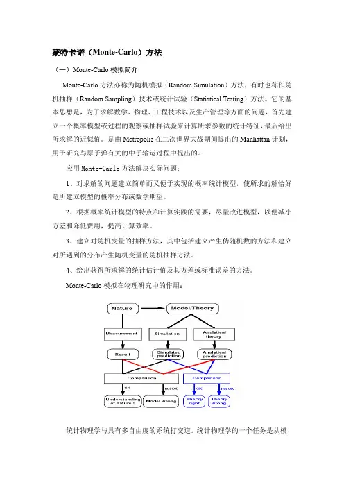
Monte-Carlo模拟在物理研究中的作用:统计物理学与具有多自由度的系统打交道。
统计物理学的一个任务是从模型的哈密顿量计算出所要的各种平均性质,例如每个自由度的平均能量E 或平均磁化强度M ,E =<H>t ∕N, M=<i iS ∑>t ∕N (2.7.1) 其中<>t 代表热平均。
A(x)表示任何可观察量,例如A=H, i i S∑等等,x 是相空间中的矢量,代表所考虑的自由度的一组变量的集合,在我们的研究范畴内,x=(12,,,N S S S ),表示系统的自旋组态。
对下式,222()()()()1x Heisenberg ij i j x ii j i x y z i i i H J S S H S S S S <>=--++=∑∑式x=(12,,,N S S S )的热平均在正则系综中由下式定义:<A(x)>T =1exp[()/]()B dx H x k T A x Z ⋅-⎰, (2.7.2) Z=exp[()/]B dx H x k T ⋅-⎰.归一化的Boltzmann 因子P(x)=1exp[()]l B x k T Z -H (2.7.3) 起着一个概率密度的作用,它描写位形x 出现在热平衡中的权重。
Monte Carlo 数值模拟法
Monte Carlo 方法亦称为随机模拟(Random simulation )方法,有时也称作随机抽样技术或统计试验方法。
基本思想是,为了求解数学、物理以及工程技术等方面的问题,首先建立一个概率模型或抽样试验来计算所求参数的统计特征,最后求出所求解的近似值,而解的精确度可以用估计值的标准差来表示。
Monte Carlo 随机模拟法被认为具有较为广泛的适用性,可以解决与随机变量有关的大量工程实际问题,在随机参数转子系统动力学响应问题分析方法中占有主导地位,其分析结果往往用来作为验证其它分析方法正确性重要指标。
Monte Carlo 随机模拟法通用性强,但是,其样本独立性问题与随机收敛性问题一直没有得到较好的解决,同时,计算工作量大,工作效率低。
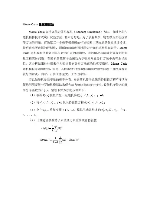
若已知随机参数变量的概率分布,根据随机转子系统的特征值方程[9]可以方便地利用蒙塔卡罗随机模拟法来研究动力响应等的统计特性。
设随机变量r 的概率分布函数为()r P x ,蒙塔卡罗方法的步骤如下:
(1)根据()r P x 模拟产生一组随机参数12,,,i i i m r r r ,i =1;
(2)将i m i i r r r ,,,21 ,i =1代入特征值方程求i
m i i w w w ,,,21 ;
(3)令i =2,3,...重复步骤(1)、(2)模拟生成足够多的12,,,i i i m w w w ,i =1,2, ,L ;
(4)计算随机参数转子系统动力响应的统计特征值
()11()L i k k i E L ωω==∑
211()(())1L i k k k i Var E L ωωω==--∑。
仿真算法知识点总结一、简介仿真算法是一种通过生成模型和运行模拟来研究系统或过程的方法。
它是一种用计算机模拟真实世界事件的技术,可以用来解决各种问题,包括工程、商业和科学领域的问题。
仿真算法可以帮助研究人员更好地理解系统的行为,并预测系统未来的发展趋势。
本文将对仿真算法的基本原理、常用技术和应用领域进行总结,以期帮助读者更好地了解和应用仿真算法。
二、基本原理1. 离散事件仿真(DES)离散事件仿真是一种基于离散时间系统的仿真技术。
在离散事件仿真中,系统中的事件和状态都是离散的,而时间是连续变化的。
离散事件仿真通常用于建模和分析复杂系统,例如生产线、通信网络和交通系统等。
离散事件仿真模型可以用于分析系统的性能、验证系统的设计和决策支持等方面。
2. 连续仿真(CS)连续仿真是一种基于连续时间系统的仿真技术。
在连续仿真中,系统中的状态和事件都是连续的,而时间也是连续的。
连续仿真通常用于建模和分析动态系统,例如电力系统、控制系统和生态系统等。
连续仿真模型可以用于分析系统的稳定性、动态特性和系统参数的设计等方面。
3. 混合仿真(HS)混合仿真是一种同时兼具离散事件仿真和连续仿真特点的仿真技术。
混合仿真可以用于建模和分析同时包含离散和连续过程的系统,例如混合生产系统、供应链系统和环境系统等。
混合仿真模型可以用于分析系统的整体性能、协调离散和连续过程以及系统的优化设计等方面。
4. 随机仿真随机仿真是一种基于概率分布的仿真技术。
在随机仿真中,系统的状态和事件都是随机的,而时间也是随机的。
随机仿真通常用于建模和分析具有随机性质的系统,例如金融系统、天气系统和生物系统等。
随机仿真模型可以用于分析系统的风险、概率特性和对策选择等方面。
5. Agent-Based ModelingAgent-based modeling (ABM) is a simulation technique that focuses on simulating the actions and interactions of autonomous agents within a system. This approach is often used for modeling complex and decentralized systems, such as social networks, biologicalecosystems, and market economies. In ABM, individual agents are modeled with their own sets of rules, behaviors, and decision-making processes, and their interactions with other agents and the environment are simulated over time. ABM can be used to study the emergent behavior and dynamics of complex systems, and to explore the effects of different agent behaviors and interactions on system-level outcomes.三、常用技术1. Monte Carlo方法蒙特卡洛方法是一种基于随机模拟的数值计算技术。


仿真是一种模拟真实系统的过程,仿真数据则是通过仿真过程产生的数据。
对于很多领域如工程、医学、科学研究等来说,仿真数据在很多时候都是非常有用的。
然而,要正确地理解和分析仿真数据并不是一件容易的事情。
在这篇文章中,我们将讨论如何正确地看懂仿真数据。
1. 了解仿真模型仿真数据是由仿真模型产生的,因此要理解仿真数据,首先需要了解仿真模型。
仿真模型是对真实系统的一种抽象和简化,它包括系统的结构、行为和动态特性等。
在理解仿真数据时,我们需要了解仿真模型的基本原理和假设条件,从而更好地理解仿真数据的产生过程和含义。
2. 确定仿真数据的类型和特征在看懂仿真数据之前,我们需要先确定仿真数据的类型和特征。
仿真数据可以是连续的时间序列数据,也可以是离散的事件数据。
仿真数据可能具有随机性和不确定性,也可能包含有周期性和趋势性。
通过对仿真数据的类型和特征进行分析,我们可以更好地选择合适的分析方法和工具,从而更准确地理解仿真数据。
3. 进行数据预处理和清洗在分析仿真数据之前,我们通常需要进行数据预处理和清洗,以确保数据的质量和可靠性。
数据预处理包括数据的去噪、缺失值处理、异常值检测和处理等。
通过数据预处理和清洗,我们可以更好地理解和分析仿真数据,避免因数据质量不佳而导致的分析错误。
4. 使用合适的分析方法和工具针对不同类型和特征的仿真数据,我们需要选择合适的分析方法和工具。
对于连续的时间序列数据,可以使用时间序列分析方法;对于具有周期性和趋势性的数据,可以使用周期性分析和趋势预测方法。
对于具有随机性和不确定性的数据,可以使用概率统计方法和模拟方法进行分析。
通过选择合适的分析方法和工具,我们可以更好地理解和分析仿真数据。
5. 结合仿真模型进行解释和验证在看懂仿真数据时,我们需要将仿真数据和仿真模型进行结合,进行数据的解释和验证。
通过将仿真数据和仿真模型进行对比和分析,我们可以更准确地理解仿真数据的含义和产生过程,从而验证仿真模型的准确性和有效性。

对海上落水人员漂流轨迹的预测研究刘凯燕【摘要】为了在海难事故发生后,在最短时间内确定遇难人员的漂移方向和位置,对海上落水人员进行受力分析,量化影响目标漂移的因素,建立海上落水人员漂移模型,并在假设初始位置误差为0以及相同的风压模型的前提下,对流场数据进行线性插值计算,增大流场数据在时间上的精确度,减小目标漂流轨迹预测的误差值.【期刊名称】《电子设计工程》【年(卷),期】2013(021)023【总页数】4页(P1-3,6)【关键词】漂移模型;蒙特卡罗法;风压模型;线性插值【作者】刘凯燕【作者单位】上海海事大学信息工程学院,上海201306【正文语种】中文【中图分类】TN919随着我国海洋经济的发展,海上遇险事故的发生也在所难免的避免。
如何在海难事故发生后尽快的找到遇难人员,减少生命损失一直都是研究的重点[1],也是我国目前海上搜救研究的难点。
海上搜救是我国根据《1979年国际海上搜寻救助公约》所承担的一项重要国际义务和一项十分重要的社会职能,也是我国履行国际义务,维护良好声誉的要求。
国内外学者对海上漂浮的漂移特性都进行了许多实验和研究。
其中,Allen A和Plourde J.V等人[2]在总结前人研究的基础上对风压作用漂浮物的运动特性进行了比较系统的研究,将海上漂浮物进行详细分类,并通过线性回归的方法建立了风压与海面10 m高处风速之间的线性经验回归方程。
Breivik等 [3]建立了挪威海和北海的搜救模型,其流场计算采用POM模式,并采用了蒙特卡洛算法确定搜寻区域,计算效果较好。
国内于卫红等[4]通过计算海流、风生流、风压差等对搜寻目标的影响,预测搜寻基准,并考虑位置或然误差、可用搜寻力量和覆盖因数等,对搜寻区域确定进行研究,建立搜寻区域确定模型,但模型是基于解析法,整体误差过大。
对此本文以落水人员为研究对象,利用粒子仿真法在计算机上模拟目标漂移的概率过程,讨论了对流场数据进行线性插值算法之后,漂移模型的误差变化。

仿真验证的常见方法仿真验证是一种帮助设计、优化和评估运行中的系统的常见方法。
它通过模拟系统的行为和性能来获得关于系统行为的详细信息,从而传达设计决策的影响和改进方案的潜在效果。
随着计算能力的提升,仿真验证已成为工程领域不可或缺的工具。
本文将介绍几种常见的仿真验证方法。
1.离散事件仿真(DES):离散事件仿真适用于模拟系统中离散事件的发生和处理过程。
它将系统建模为由一系列事件组成的网络,每个事件代表一个系统状态的改变。
通过模拟事件的发生和处理过程,离散事件仿真可以帮助评估不同的决策方案对系统性能的影响。
2.连续仿真(CS):连续仿真适用于模拟连续系统的行为。
它将系统建模为一组连续的方程和约束条件,并使用数值方法来模拟系统的运行。
连续仿真在评估系统的动态性能和响应性方面非常有用。
3. 蒙特卡罗仿真(Monte Carlo Simulation):蒙特卡罗仿真是一种基于随机抽样的方法,用于评估系统在不同参数组合下的行为和性能。
它通过从概率分布中抽取大量样本,利用这些样本的统计特性来估计系统的行为。
蒙特卡罗仿真可以帮助评估系统的风险和不确定性。
4. Agent-Based Modeling(ABM):Agent-Based Modeling是一种建立于个体行为的仿真方法。
它将系统建模为一组独立的个体,每个个体都有自己的行为规则和互动方式。
通过模拟个体之间的互动,Agent-Based Modeling可以帮助评估不同决策对系统整体行为的影响。
5. 虚拟现实仿真(Virtual Reality Simulation):虚拟现实仿真是一种基于计算机生成的环境和交互技术的仿真方法。
它通过模拟真实场景和用户交互,提供一种沉浸式的仿真体验。
虚拟现实仿真可以帮助评估设计决策在真实环境中的效果和用户体验。
6. 博弈论仿真(Game Theory Simulation):博弈论仿真是一种用于评估决策者之间策略选择和博弈行为的仿真方法。


随机车流荷载模拟方法及应用研究作者:张杰耿波来源:《科教导刊·电子版》2013年第23期摘要通过采集过桥交通流荷载数据,确定影响车流荷载随机特性的参数。
从车型、车重、车道分布、车间距出发设计,模拟随机车流。
将模拟的车流荷载加载与桥梁单元应力影响线得到应力历程,通过雨流计数法得到模拟的应力谱,比较模拟应力谱与实测应力谱,验证荷载模拟在疲劳分析中的可用性。
关键词随机车流随机特性参数应力谱中图分类号:U441.2 文献标识码:A1概述对随机车流的分析总体上分三个阶段:以随机过程为理论基础的模拟分析阶段;静态交通流模拟;动态交通流模拟。
对于桥梁结构的车流荷载,通常假定车流是既定的,而忽略车流荷载的随机特性,这导致分析所得结论偏离实际情况。
随着研究的深入,开始考虑车辆荷载参数的随机性,充分调查交通荷载状况,通过统计分析交通流的各个参数,综合模拟接近运营状态的车辆交通流,应用于桥梁结构的安全性评估中。
对随机车流荷载进行合理恰当的模拟对计算结果的准确性和可靠性都有很大的提升,以便更科学地指导工程实践。
由于交通运输的发展,车辆荷载逐年增加,另一方面桥梁运营时间增加,所以对现有桥梁的剩余寿和安全性进行重新分析评估,已成为较为紧迫的突出问题。
对表征随机车流复杂性的各因素的研究,通过研究合理模拟随机车流是准确科学评估桥梁剩余寿命的重中之重。
桥梁通行车流受到路况、车况、当地经济环境及天气状况等众多因素影响,是一个复杂的随机过程。
在建立数学模型的过程中主要以车型、车道、车间距,车重几为参数。
研究表明车型、车道服从均匀分布;车重服从极值I型分布,车间距服从对数正态分布;根据观测数据的统计参数,进行参数估计,利用数理统计与随机过程的理论方法实现随机车流模拟。
在交通荷载的调查基础上,通过动态交通流模拟,预测交通量,可降低工程项目成本。
对于桥梁工程,随机车流的模拟可以更恰当合理地反映作用于桥梁上的实际车辆荷载,使得桥梁结构的疲劳寿命分析更加科学可靠。
统计方法4 随机模拟随机模拟(random simulation)方法,又称为蒙特卡洛(Monte Carlo,MC )方法。
它的基本思想是为了求解实践中问题,首先建立一个概率模型或随机过程,使它的参数等于问题的解,然后通过对模型的抽样试验获得这些参数的统计特征,最后给出解的近似值。
解的精确度由估计值得标准误差来表示。
其基本数学原理为强大数定律。
Monte Carlo 方法最早产生于二战期间美国研发原子弹的曼哈顿工程。
电子计算机的出现使得模拟随机试验成为了重要的科学方法。
图:赌城Monte CarloMonte Carlo 方法可以处理的问题基本可以可以分为两类:第一类是随机性的问题。
这一类问题往往直接利用概率法则通过随机抽样进行模拟。
如核物理问题,随机服务系统中的排队问题,生物种群的繁衍与竞争,传染病的传播等都属于这一问题。
第二类是确定性的问题。
首先建立一个与所求问题有关的概率模型,使所求解是该概率模型中的概率分布或者数学期望。
然后对这个模型进行随机抽样。
用算术平均值作为所求解的估计值。
如求解多重积分,解线性方程组,解偏微分方程积分方程等复杂数学问题。
第一节 生成随机数 1.生成随机数的基本数学原理较为普遍应用的产生随机数的方法是选取一个函数)(x g ,使其将整数变换为随机数。
以某种方法选取0x ,并按照)(1k k x g x =+产生下一个随机数。
最一般的方程)(x g 具有如下形式:c ax x g mod)()(+= (8.1)其中0x 初始值或种子(00>x )=a 乘法器(0≥a )=c 增值(0≥c )=m 模数对于t 数位的二进制整数,其模数通常为t 2。
例如,对于31位的计算机m 即可取1312-。
这里a x ,0和c 都是整数,且具有相同的取值范围0,,x m c m a m >>>。
所需的随机数序{}n x 便可由下式得m c ax x n n mod )(1+=+ (8.2) 该序列称为线性同余序列。
随机模拟法在仿真航班计划生成中的应用作者:高伟张腾飞来源:《科技创新导报》 2014年第2期高伟张腾飞(中国民航大学空中交通管理学院天津东丽 300300)摘要:针对空域容量评估工作对仿真航班计划的要求,以航班计划的流量分布统计特征为约束条件,建立数学模型,采用随机模拟法作为求解该问题的方法。
经过多次仿真,并对仿真结果进行分析,分析结果表明:随机模拟法解决复杂的、不确定性问题的优势,可以快速有效地解决仿真航班计划生成问题,生成的仿真航班计划各项流量统计特征均能满足要求,生成仿真航班计划的方法具有很强的稳定性和实用性。
关键词:随机模拟法航班计划航班元素统计特征中图分类号:TP31 文献标识码:A 文章编号:1674-098X(2014)01(b)-0089-04Research on the application of stochastic simulation in generation ofsimulation flight planGAO Wei,ZHANG Teng fei(College of air traffic management, Civil Aviation University of China, Dongli Tianjin 300300, China)Abstract:The paper aimed at the requirements for simulation flight plan in the airspace capacity evaluation work,sets up a mathematics model according to the flow and pivotal property statistical characteristics of flight plan,the stochastic simulation method is used to solve the problem.For simulatingmany times,the simulation results is analyzed,the results shows that:the advantages of stochastic simulation method that solve complex and uncertainty problem can effectively solve the problem of generating simulation flight plan,the various flow statistical characteristics can meet the requirements,the method has strong stability and practicability.Key Words:stochastic simulation flight plan flight elements statistical characteristics我国经济的快速发展,对民航运输提出了新的要求,全国各主要机场通过改扩建或者增加航班架次等方式来提高运力运量,这就需要对运量提升进行容量评估。
10随机模拟只要你自己试试模拟随机现象几次,就会加强对概率的了解,比读很多页的数理统计和概率论的文章还有用。
学习模拟,不仅是为了解模拟本身,也是为更了解概率而了解模拟。
10.1伪随机数生成(0,1)之间均匀分布的伪随机数的函数为uniform()di uniform()di uniform()di uniform()每次都得到一个大于零小于1的随机数。
如果要生成一位数的随机数(即0,1,2,3,4,5,6,7,8,9),可以取小数点后第一位数,通常用下面的命令di int(10*uniform())两位随机数(0-99)则取小数点后两位小数,即也可以同时生成多个随机数,然后将该随机数赋给某个变量。
要注意的是,电脑中给出的随机数不是真正的随机数,而是伪随机数,因为它是按照一定的规律生成的。
如果给定基于生成伪随机数的初始数值(即set seed #),则对相同的初始数值,生成的伪随机数序列完全一样。
*============================begin====================================clearset obs 10gen x1=uniform()gen x2=uniform() //注意到x1与x2不一样set seed 1234gen y1=uniform()set seed 1234gen y2=uniform()gen y3=uniform() //注意到y1与y2一样,但均与y3不同set seed 5634gen z1=uniform()set seed 1234gen z2=uniform()//注意到z2与y1,y2一样,但z1与z2不同list*============================end====================================10.2简单模拟一旦有了可靠的概率模型,模拟是找出复杂事件发生概率的有效工具。
组合信用损失分布的蒙特卡洛模拟孙云龙,陈伶俐(西南财经大学经济数学学院,成都610074)摘要:组合损失分布的确定是测量各种组合信用风险的一个先决条件.本文通过对信用风险损失理论进行分析的基础上,分析阐述了利用蒙特卡罗方法模拟组合信用损失的原理和方法,并基于Matla b语言结合实际问题进行仿真实验,实验结果表明该模拟方法能较好地反映组合信用损失的分布特征,具有有效性和实用性.中图分类号:O242 . 1 ; F830 . 9文献标志码: A信用风险是金融风险管理的重点,在组合信用风险管理中,组合损失分布的确定又是测量各种组合信用风险(比如资产组合的在险价值Va R) 的一个先决条件. 使用Cre d it Met ric s , KMV , C re d it ri s k + 以及Credit2 Po r tfolio View ( C PV) 等现代信用管理模型来测度信用风险时,组合信用损失分布均是计算的基础. 对于风险管理的模型研究大多采用概率统计理论的分析方法,但投资组合种类繁多时,如资产数为n Ε10 ,那违约事件的种类就有2 n Ε1 024 种,计算违约事件概率就非常繁琐,必须借助数值方法来获得其近似值,因此蒙特卡罗模拟方法便成为计算组合损失分布的有效方法,甚至是首选方法.近年来,国内学者对现代信用风险测度技术的研究方兴未艾,一些学者对信用风险的模拟技术进行了研究,但相关文献较少,并且不够详实、全面. 本文通过对信用风险损失理论进行分析的基础上,分析阐述组合信用损失的蒙特卡罗模拟原理与方法,并基于Mat l a b语言进行了仿真实验,结合实际问题进行验证分析得1信用风险的度量信用风险是债务人到期不能履约的风险.这里所关注的焦点是“违约”事件的发生,以及违约的发生给债权人带来的损失. 但在债务人违约前,如果债务人的信用状况恶化.那债务人违约可能性就增加了,那么,即使还没有违约,债权人承受的违约风险也加大了,应该得到更高的风险升水作为补偿,而这意味着其债权的贬值. 因此,可以将信用风险广义地理解为债务人违约可能性的加大给债权人带来的债权贬值的风险. 与传统狭义的理解不同,这一理解不是仅仅关注违约事件的发生,而是还关心债务人违约可能性的变化,尤其是违约可能性的上升,因为这会导致债权人的资产价值上发生更大的损失. 这里考虑的信用风险为交易对手违约或信用品质潜在变化而导致发生损失的可能性.先考虑由违约形成的信用风险.由这种债务所形成组合的信用风险引起的损失可以表示为:N NL C = ∑b i ×L i = ∑b i ×C E i ×(1 - f i ) ,(1)i = 1 i = 1其中:L C 表示整个债务组合由信用风险引发的损失;债务组合的数量为N ; b i 是违约概率为p i 的随机变量,如果违约发生,该变量取值为1 ,否则取值为0 ,有E[ b i ] = p i ; L j 是其中第j 种事件发生时的损失; C E i 是违约发生时的信用风险暴露; f i 表示回收率,那1 - f i 为违约发生时的损失率.假设只有b i , i = 1 ,2 , ⋯, N 是随机变量,则由式(1) 得信用损失的期望值为:N N∑E ( b i)∑pi×CE i ×( 1 - f i ) . ×CE i ×( 1 - f i ) ( 2)E[ L C ] ==i = 1i = 1信用损失的波动性 ( 方差) 在很大程度上依赖于发生违约事件之间的相关性 , 信用损失的方差为 :NNva r [ L C ] ∑∑( Li- E ( L i ) ) ( L jE ( L j ) ) p ij , ( 3)=- i = 1 j = 1其中 p ij 为第 i 及 j 事件同时发生的概率 , 显然 , 信用损失的方差不仅与单个违约事件的方差有关 , 与违约事 件间的相关性有关.组合信用风险的蒙特卡洛模拟分析蒙特 卡 洛 ( Mo nt eCa rlo ) 法 亦 称 为 随 机 模 拟 ( ra ndmo n si mulatio n ) 方 法 , 有 时 也 称 作 随 机 抽 样( ra ndo m sa mp li ng ) 技术或统计试验 ( st ati sticalt e sti ng ) 方法 . 它是一种与一般数值计算方法有本质区别的计算方法 ,属于试验数学的一个分支 ,起源于早期的用几率近似概率的数学思想 ,它利用随机数进行统计试验 , 以求得的统计特征值 (如均值 、概率等) 作为待解问题的数值解. 蒙特卡洛模拟方法已经成为金融分析中不 可或缺的重要方法.利用蒙特卡罗方法模拟组合信用损失分布的一般步骤如下 :2 . 1数据准备通过对资产组合的分析得到相关基础数据 :( 1) 根据资产组合中各个债务项目的信用评级 , 由相关信用评级机构 ( 如标准普尔 、穆迪等) 统计结果得到各个资产的违约概率值 p i ;2ρ121⋯ ρ2 n⋯ ⋯ ρ1 nρ2 n ⋯ 1 1ρ12⋯ ρ1 n R =.⋯ 2 . 2 违约事件模拟由多元正态分布的定义可以推出以下定理[ 8 ] :设 X = ( X 1 , X 2 , ⋯, X n ) T 为独立标准正态变量 , 则随机变量 : Y = A T X 服从 n 维正态分布 N (μ,定理 T∑) , 其中∑= A A .利用矩阵分解方法 , 产生具有相关性的多元正态随机数 , 模拟组合信用风险的损失值 :( 1) 将相关系数矩阵 R 进行分解 ( Chole s ky 分解 、特征值分解 、奇异值分解等) , 得到矩阵 A 满足 :R = A A T.( 2) 计算违约分位点 z i :P ( y i < z i ) = p i .( 3) 产生信用相关的多变量随机数 :首先生成 N 个服从标准正态分布随机数 X = ( X 1 , X 2 , ⋯, X n ) T , 则 :Y = A TX为具有相关系数 R 的随机向量.( 4) 通过判断得到 N 项债务组合的违约是否发生的数量 0 - 1 变量 : b = ( b 1 , b 2 , ⋯, b n )1 , Y i Φ z i ,b i = 0 , Y i Ε z i .2 .3 得到信用损失分布(1) 通过违约事件模拟计算信用损失N NL C = ∑b i ×L i= ∑b i ×CE i×(1- f i ) .i = 1 i = 1(2) 重复(1) 若干次(比如m = 10 万次) ,即可得到m 个不同情景下的组合损失. 将m 个组合损失分类汇总,得到信用损失的概率分布列表,计算均值、方差等.由于分类项目较多,一般可用图形显示组合信用损失分布.2 .4 根据信用损失分布进行风险分析由于通过模拟得到了组合信用损失分布,便可进行进一步分析. 例如:可根据给定的置信水平得到Va R 值.3实例分析现以一个银行贷款为例,使用M a t l ab 软件编程求解,计算信用损失分布,并根据信用损失分布进行风险分析.3 .1 问题提出假设银行贷款的总值为100 万元,分别投资于10 个企业A1 , A2 , ⋯, A10 ,利用穆迪公司的评级方法对企业进行评级,各种企业的评级、年份、违约暴露,以及根据穆迪公司统计的各种债券级别的历史违约率如下表.债券穆迪公司评级第几年违约暴露/ 万元违约概率/ % 违约回收率A1 A2 A3 A4 A5 A6 A7 A8 A9A A AA A AAaAa AABaaBaaBa8102641379312966112281050 . 180 . 240 . 150 . 360 . 350 . 470 . 880 . 912 . 170 . 750 . 710 . 680 . 600 . 520 . 470 . 390 . 350 . 28A 10B 4 11 4 . 55 0 . 16 根据这10 个企业历史收益的相关性,得到它们的该资产组合的违约相关矩阵为:1 . 000 0 0 . 373 4 0 . 029 8 0 . 130 0 0 . 112 5 0 . 072 8 0 . 138 4 0 . 160 5 0 . 147 4 0 . 215 2 0 . 373 41 . 000 00 . 349 10 . 250 60 . 194 60 . 721 10 . 336 20 . 243 00 . 052 40 . 478 20 . 029 80 . 349 11 . 000 00 . 087 80 . 358 00 . 322 70 . 458 10 . 330 30 . 418 10 . 586 40 . 130 00 . 250 60 . 087 81 . 000 00 . 770 00 . 677 20 . 138 90 . 699 60 . 346 70 . 116 30 . 112 50 . 194 60 . 358 00 . 770 01 . 000 00 . 622 50 . 345 50 . 798 80 . 244 20 . 535 70 . 072 80 . 721 10 . 322 70 . 677 20 . 622 51 . 000 00 . 323 40 . 527 20 . 228 80 . 305 90 . 138 40 . 336 20 . 458 10 . 138 90 . 345 50 . 323 41 . 000 0- 0 . 06 10- 0 . 131 30 . 316 30 . 160 50 . 243 00 . 330 30 . 699 60 . 798 80 . 527 2- 0 . 06 01 . 000 00 . 172 60 . 503 40 . 147 40 . 052 40 . 418 10 . 346 70 . 244 20 . 228 8- 0 . 131 30 . 172 61 . 000 0- 0 . 046 10 . 215 20 . 478 20 . 586 40 . 116 30 . 535 70 . 305 90 . 316 30 . 503 4- 0 . 046 11 . 000 0r =试计算信用损失分布,并求此投资组合的Va R.3 .2 模型求解基于Mat l a b强大的运算功能,本文将在Mat l a b软件下进行蒙特卡洛分析,主要按照如下步骤进行:(1) 输入违约概率值p 、资产回收率f 、相关系数矩阵r.(2) 使用chol 函数对相关系数矩阵进行分解.(3) 利用Mat la b 编程,使用ra ndn 函数,模拟投资组合1 000 000 次,产生具有相关性的多变量随机数, 计算组合信用风险的损失值,计算各种损失频率,得到信用损失分布列,将信用损失分布用图形表示如下(见图1) .从图中可以看出,损失分布并不是单调增长的,主要集中在0 万、3 . 6 万、4 . 9 万、6 . 5 万、9 . 2 万、11 . 7 、15 . 7 万等几个点上.(4) 计算Va R计算信用损失累积概率分布,其图形如图2 .给定置信度为95 % ,利用已模拟的信用损失分布列,可得信结论4通过以上分析可以看出,利用蒙特卡洛方法模拟资产组合的信用损失分布,能较好地反映组合损失的分布特征,解决了资产组合包含大量资产时信用风险损失分布的估计问题,在此基础上可以根据需要进一步讨论信用风险的各种度量分析. 通过多次模拟实验显示,模拟结果数据稳定,表明该方法具有有效性和实用性.参考文献[ 1 ] 魏丽. 风险投资和大额索赔下更新模型的破产概率[J ] . 中国科学A 辑:数学,2009 ,39 ( 8) :9332938 .[ 2 ] 陈德胜,冯宗宪. 资产组合信用风险度量技术比较研究—基于V A R[J ] . 经济问题研究,2005 ,255 ( 2) :38243 .[ 3 ] Pat ricia J ack s o n , Willia m Per r audi n. regulato r y i m plicatio n s of Credit ri s k Mo d eli n g [J ] . J o u r n al of Ban k i n g &Fi n a n ce ,2004 ( 24) :1214 . [ 4 ] A r n a u d de Ser v igny . Mea s uri n g a n d Ma n agi n g Credit Ri s k [ M ] . New Y o r k : Mc Graw2Hill , 2004 : 2132251 .[ 5 ] 沈沛龙,任若恩,马杰. 我国商业银行信用风险的度量与控制[ J ] . 北京航空航天大学学报:社会科学版,2000 ,13 ( 04) :56260 .[ 6 ] 喻波,王慧. 新巴塞尔协议框架与Va R方法的运用[J ] . 财经科学,2004 ( 6) :87291 .[ 7 ] Ru s sel E Cafli s ch . Mo n t e Ca r lo qua s i 2Mo n t e Ca r lo met ho d s[J ] . Act a N u m erica ,1998 ,7 :1249 .[ 8 ] 张尧庭,方开泰. 多元统计分析引论[ M ] . 北京:科学出版社,1999 :652118 .Monte C arl o Simulat i on of Credit Loss Distribut i on of Portf ol ioSU N Yun2lo ng ,C H EN L i n2li( School of Fi n a n ce a n d Eco n o mics , S o u t hwe s t e r n U n iver s it y , Chengdu 610074 , C hi n a)Abstract : Identificatio n fo r credit lo ss di st ributio n of po rtfolio i s p rerequi site to mea sure t he credit lo ss. The a rticle ex2 plains t he p rinciple s a nd met ho ds of simulati ng t he di st ri butio n of po rtfolio’s credit lo ss wit h Mo nte Ca rlo met ho d , o n t he ba si s of analysi s o n t he t heo ry of credit lo ss. Matlab i s used to ca r r y o ut t he experimental simulatio n , t he re sult of w hich sho w s t he validit y and p ractica b ilit y of t he met ho d.K ey w ords : mea s uring credit ri s k ; credit Lo ss di s t ri b utio n ; Mo n te Ca r lo simulatio n ; Chole s ky deco mpo sitio n ; Matla b。