A Multivariate Poisson-Lognormal Regression Model for Prediction of Crash Counts by Severit

概率密度估计
1 概率密度估计
概率密度估计（Probability Density Estimation，简称PDE）也称为密度函数估计，旨在描述一个随机变量X的概率密度函数，从而
帮助准确定量分析研究变量X的特征。

通常，概率密度估计的过程可以分解为两个步骤。

第一步是从样
本中提取该变量的直方图，然后以某种函数形式拟合该直方图，得到
其对应的概率密度函数。

其中，最常用的函数形式为高斯分布（Gaussian Distribution）的普通分布、泊松分布（Poisson Distribution）、多元正态分布（Multivariate Normal Distribution）、双截止分布（Binomial Distribution）、逻辑正态
分布（Log-normal Distribution）等。

第二步就是根据拟合出概率密度函数形状，运用其特点和参数，
得到该变量的最佳估计，便于对样本进行更有效率的分析。

比如，在
高斯分布模型下，样本拟合出的方差可以帮助我们判断数据的稳定性。

概率密度估计被广泛应用于贝叶斯统计分析、学习理论、社会科
学研究等，是发现重要模式并探寻变量分布的重要工具。

总之，概率密度估计是一项核心重要的数据分析技术，其解释力、拟合能力和模型大小的理论基础为研究者们收集总结数据，比较复杂
的变量特征提供了可靠信息。

统计学复试专业词汇汇总population 总体sampling unit 抽样单元sample 样本observed value 观测值descriptive statistics 描述性统计量random sample 随机样本simple random sample 简单随机样本statistics 统计量order statistic 次序统计量sample range 样本极差mid-range 中程数estimator 估计量sample median 样本中位数sample moment of order k k阶样本矩sample mean 样本均值average 平均数arithmetic mean 算数平均值sample variance 样本方差sample standard deviation 样本标准差sample coefficient of variation 样本变异系数standardized sample random variable 标准化样本随机变量sample coefficient of skewness （歪斜）样本偏度系数sample coefficient of kurtosis (峰态) 样本峰度系数sample covariance 样本协方差sample correclation coefficient 样本相关系数standard error 标准误差interval estimator 区间估计statistical tolerance interval 统计容忍区间statistical tolerance limit 统计容忍限confidence interval 置信区间one-sided confidence interval 单侧置信区间prediction interval 预测区间estimate 估计值error of estimation 估计误差bias 偏倚unbiased estimator 无偏估计量maximum likelihood estimator 极大似然估计量estimation 估计maximum likelihood estimation 极大似然估计likelihood function 似然函数profile likelihood funtion 剖面函数hypothesis 假设null hypothesis 原假设alternative hypothesis 备择假设simple hypothesis 简单假设composite hypothesis 复合假设significance level 显著性水平type I error 第一类错误type II error 第二类错误statistical test 统计检验significance test 显著性检验p-value p值power of a test 检验功效power curve 功效曲线test statistic 检验统计量graphical descriptive statistics 图形描述性统计量numerical descriptive statistics 数值描述性统计量classes 类（组）class 类class 组class limits; class boundaries 组限mid-point of class 组中值class width 组距frequency 频数frequency distribution 频数分布histogram 直方图bar chart 条形图cumulative frequency 累积频数relative frequency 频率cumulative relative frequency 累积频率sample space 样本空间event 事件complementary event 对立事件independent events 独立事件probability [of an event A] [事件A的]概率conditional probability 条件概率distribution function [of a random variable X] [随机变量X的]分布函数family of distributions 分布族parameter 参数random variable 随机变量probability distribution 概率分布distribution 分布expectation 期望p-quantile; p-fractile p分位数median 中位数quartile 四分位数univariate probability distribution 一维概率分布univariate distribution 一维分布multivariate probability distribution 多维概率分布multivariate distribution 多维分布marginal probability distrubition 边缘概率分布marginal distribution 边缘分布conditional probability distribution 条件概率分布conditional distribution 条件分布regression curve 回归曲线regression surface 回归曲面discrete probability distribution 离散概率分布discrete distribution 离散分布continuous probability distribution 连续概率分布continuous distribution 连续分布probability [mass] function 概率函数mode of probability [mass] function 概率函数的众数probability density function 概率密度函数mode of probability density function 概率密度函数的众数discrete random variable 离散随机变量continuous random variable 连续随机变量centred probability distribution 中心化概率分布centred random variable 中心化随机变量standardized probability distribution 标准化概率分布standardized random variable 标准化随机变量moment of order r r阶[原点]矩means 均值moment of order r = 1 一阶矩mean 均值variance 方差standard deviation 标准差coefficient of variation 变异系数coefficient of skewness 偏度系数coefficient of kurtosis 峰度系数joint moment of order r and s (r,s)阶联合[原点]矩joint central moment of order r and s (r,s)阶联合中心矩covariance 协方差correlation coefficient 相关系数multinomial distribution 多项分布binomial distribution 二项分布Poisson distribution 泊松分布hypergeometric distibution 超几何分布negative binomial distribution 负二项分布normal distribution, Gaussian distribution 正态分布standard normal distribution, standard Gaussian distribution 标准正态分布lognormal distribution 对数正态分布t distribution; Student's distribution t分布degrees of freedom 自由度F distribution F分布gamma distribution 伽玛分布, Γ分布chi-squared distribution 卡方分布,χ2分布exponential distribution 指数分布beta distribution 贝塔分布,β分布uniform distribution, rectangular distribution 均匀分布type I value distribution; Gumbel distribution I型极值分布type II value distribution; Gumbel distribution II型极值分布Weibull distribution 威布尔分布type III value distribution; Gumbel distribution III型极值分布multivariate normal distribution 多维正态分布bivariate normal distribution 二维正态分布standard bivariate normal distribution 标准二维正态分布sampling distribution 抽样分布probability space 概率空间。

二维高斯混合分布参数估计python -回复二维高斯混合分布是一种常用的概率模型，常用于数据聚类、模式识别等领域。

在实际应用中，估计二维高斯混合分布的参数是十分重要的一项任务。

本文以Python为工具，并结合实例，介绍了如何一步一步地估计二维高斯混合分布的参数。

1. 引言二维高斯混合分布常用于将数据集拟合到一组由多个二维高斯分布组成的模型中。

通过估计混合分布的参数，我们可以了解数据集的特征和结构，从而进行数据分类、聚类和模式识别等任务。

在本文中，我们将通过以下步骤来估计二维高斯混合分布的参数：1. 初始化参数2. Expectation-Maximization（EM）算法3. 参数优化4. 数据聚类让我们一起开始吧！2. 初始化参数在估计二维高斯混合分布的参数之前，我们首先需要初始化一些参数。

常用的参数包括：- K：混合分布的组数- μ：各组的均值向量- Σ：各组的协方差矩阵- α：各组的权重我们可以使用随机数来初始化均值向量μ和协方差矩阵Σ，而权重α可以初始化为均匀分布。

下面是一个Python函数来实现参数的初始化：pythonimport numpy as npdef initialize_parameters(data, num_clusters):num_dimensions = data.shape[1]mu = np.random.randn(num_clusters, num_dimensions)sigma = [np.eye(num_dimensions)] * num_clustersalpha = np.ones(num_clusters) / num_clustersreturn mu, sigma, alpha注意，我们假设数据集已经加载到名为`data`的Numpy数组中，并且`num_clusters`是我们想要估计的高斯混合分布组数。

3. Expectation-Maximization算法Expectation-Maximization（EM）算法是一种常用的参数估计方法，特别适用于高斯混合分布。

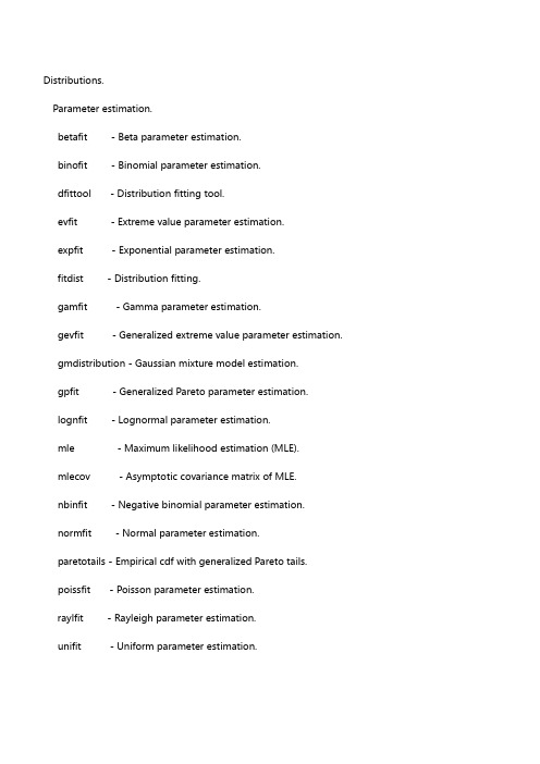
Distributions.Parameter estimation.betafit - Beta parameter estimation.binofit - Binomial parameter estimation.dfittool - Distribution fitting tool.evfit - Extreme value parameter estimation.expfit - Exponential parameter estimation.fitdist - Distribution fitting.gamfit - Gamma parameter estimation.gevfit - Generalized extreme value parameter estimation.gmdistribution - Gaussian mixture model estimation.gpfit - Generalized Pareto parameter estimation.lognfit - Lognormal parameter estimation.mle - Maximum likelihood estimation (MLE).mlecov - Asymptotic covariance matrix of MLE.nbinfit - Negative binomial parameter estimation.normfit - Normal parameter estimation.paretotails - Empirical cdf with generalized Pareto tails.poissfit - Poisson parameter estimation.raylfit - Rayleigh parameter estimation.unifit - Uniform parameter estimation.wblfit - Weibull parameter estimation. Probability density functions (pdf).betapdf - Beta density.binopdf - Binomial density.chi2pdf - Chi square density.evpdf - Extreme value density.exppdf - Exponential density.fpdf - F density.gampdf - Gamma density.geopdf - Geometric density.gevpdf - Generalized extreme value density. gppdf - Generalized Pareto density.hygepdf - Hypergeometric density.lognpdf - Lognormal density.mnpdf - Multinomial probability density function. mvnpdf - Multivariate normal density.mvtpdf - Multivariate t density.nbinpdf - Negative binomial density.ncfpdf - Noncentral F density.nctpdf - Noncentral t density.ncx2pdf - Noncentral Chi-square density. normpdf - Normal (Gaussian) density.pdf - Density function for a specified distribution.poisspdf - Poisson density.raylpdf - Rayleigh density.tpdf - T density.unidpdf - Discrete uniform density.unifpdf - Uniform density.wblpdf - Weibull density.Cumulative Distribution functions (cdf).betacdf - Beta cumulative distribution function.binocdf - Binomial cumulative distribution function.cdf - Specified cumulative distribution function.chi2cdf - Chi square cumulative distribution function.ecdf - Empirical cumulative distribution function (Kaplan-Meier estimate).evcdf - Extreme value cumulative distribution function.expcdf - Exponential cumulative distribution function.fcdf - F cumulative distribution function.gamcdf - Gamma cumulative distribution function.geocdf - Geometric cumulative distribution function.gevcdf - Generalized extreme value cumulative distribution function.gpcdf - Generalized Pareto cumulative distribution function.hygecdf - Hypergeometric cumulative distribution function.logncdf - Lognormal cumulative distribution function.mvncdf - Multivariate normal cumulative distribution function. mvtcdf - Multivariate t cumulative distribution function. nbincdf - Negative binomial cumulative distribution function. ncfcdf - Noncentral F cumulative distribution function.nctcdf - Noncentral t cumulative distribution function.ncx2cdf - Noncentral Chi-square cumulative distribution function. normcdf - Normal (Gaussian) cumulative distribution function. poisscdf - Poisson cumulative distribution function.raylcdf - Rayleigh cumulative distribution function.tcdf - T cumulative distribution function.unidcdf - Discrete uniform cumulative distribution function. unifcdf - Uniform cumulative distribution function.wblcdf - Weibull cumulative distribution function.Critical Values of Distribution functions.betainv - Beta inverse cumulative distribution function.binoinv - Binomial inverse cumulative distribution function.chi2inv - Chi square inverse cumulative distribution function. evinv - Extreme value inverse cumulative distribution function. expinv - Exponential inverse cumulative distribution function. finv - F inverse cumulative distribution function.gaminv - Gamma inverse cumulative distribution function.geoinv - Geometric inverse cumulative distribution function.gevinv - Generalized extreme value inverse cumulative distribution function.gpinv - Generalized Pareto inverse cumulative distribution function.hygeinv - Hypergeometric inverse cumulative distribution function.icdf - Specified inverse cumulative distribution function.logninv - Lognormal inverse cumulative distribution function.nbininv - Negative binomial inverse distribution function.ncfinv - Noncentral F inverse cumulative distribution function.nctinv - Noncentral t inverse cumulative distribution function.ncx2inv - Noncentral Chi-square inverse distribution function.norminv - Normal (Gaussian) inverse cumulative distribution function.poissinv - Poisson inverse cumulative distribution function.raylinv - Rayleigh inverse cumulative distribution function.tinv - T inverse cumulative distribution function.unidinv - Discrete uniform inverse cumulative distribution function.unifinv - Uniform inverse cumulative distribution function.wblinv - Weibull inverse cumulative distribution function.Random Number Generators.betarnd - Beta random numbers.binornd - Binomial random numbers.chi2rnd - Chi square random numbers.evrnd - Extreme value random numbers.exprnd - Exponential random numbers.frnd - F random numbers.gamrnd - Gamma random numbers.geornd - Geometric random numbers.gevrnd - Generalized extreme value random numbers.gprnd - Generalized Pareto inverse random numbers.hygernd - Hypergeometric random numbers.iwishrnd - Inverse Wishart random matrix.johnsrnd - Random numbers from the Johnson system of distributions. lognrnd - Lognormal random numbers.mhsample - Metropolis-Hastings algorithm.mnrnd - Multinomial random vectors.mvnrnd - Multivariate normal random vectors.mvtrnd - Multivariate t random vectors.nbinrnd - Negative binomial random numbers.ncfrnd - Noncentral F random numbers.nctrnd - Noncentral t random numbers.ncx2rnd - Noncentral Chi-square random numbers.normrnd - Normal (Gaussian) random numbers.pearsrnd - Random numbers from the Pearson system of distributions. poissrnd - Poisson random numbers.randg - Gamma random numbers (unit scale). random - Random numbers from specified distribution. randsample - Random sample from finite population. raylrnd - Rayleigh random numbers.slicesample - Slice sampling method.trnd - T random numbers.unidrnd - Discrete uniform random numbers.unifrnd - Uniform random numbers.wblrnd - Weibull random numbers.wishrnd - Wishart random matrix.Quasi-Random Number Generators.haltonset - Halton sequence point set.qrandstream - Quasi-random stream.sobolset - Sobol sequence point set.Statistics.betastat - Beta mean and variance.binostat - Binomial mean and variance.chi2stat - Chi square mean and variance.evstat - Extreme value mean and variance.expstat - Exponential mean and variance.fstat - F mean and variance.gamstat - Gamma mean and variance.geostat - Geometric mean and variance.gevstat - Generalized extreme value mean and variance. gpstat - Generalized Pareto inverse mean and variance. hygestat - Hypergeometric mean and variance. lognstat - Lognormal mean and variance.nbinstat - Negative binomial mean and variance. ncfstat - Noncentral F mean and variance.nctstat - Noncentral t mean and variance.ncx2stat - Noncentral Chi-square mean and variance. normstat - Normal (Gaussian) mean and variance. poisstat - Poisson mean and variance.raylstat - Rayleigh mean and variance.tstat - T mean and variance.unidstat - Discrete uniform mean and variance.unifstat - Uniform mean and variance.wblstat - Weibull mean and variance.Likelihood functions.betalike - Negative beta log-likelihood.evlike - Negative extreme value log-likelihood. explike - Negative exponential log-likelihood. gamlike - Negative gamma log-likelihood.gevlike - Generalized extreme value log-likelihood.gplike - Generalized Pareto inverse log-likelihood. lognlike - Negative lognormal log-likelihood.nbinlike - Negative binomial log-likelihood.normlike - Negative normal likelihood.wbllike - Negative Weibull log-likelihood.Probability distribution objects.ProbDistUnivKernel - Univariate kernel smoothing distributions. ProbDistUnivParam - Univariate parametric distributions. Descriptive Statistics.bootci - Bootstrap confidence intervals.bootstrp - Bootstrap statistics.corr - Linear or rank correlation coefficient.corrcoef - Linear correlation coefficient (in MATLAB toolbox). cov - Covariance (in MATLAB toolbox).crosstab - Cross tabulation.geomean - Geometric mean.grpstats - Summary statistics by group.harmmean - Harmonic mean.iqr - Interquartile range.jackknife - Jackknife statistics.kurtosis - Kurtosis.mad - Median Absolute Deviation.mean - Sample average (in MATLAB toolbox).median - 50th percentile of a sample (in MATLAB toolbox).mode - Mode, or most frequent value in a sample (in MATLAB toolbox). moment - Moments of a sample.nancov - Covariance matrix ignoring NaNs.nanmax - Maximum ignoring NaNs.nanmean - Mean ignoring NaNs.nanmedian - Median ignoring NaNs.nanmin - Minimum ignoring NaNs.nanstd - Standard deviation ignoring NaNs.nansum - Sum ignoring NaNs.nanvar - Variance ignoring NaNs.partialcorr - Linear or rank partial correlation coefficient.prctile - Percentiles.quantile - Quantiles.range - Range.skewness - Skewness.std - Standard deviation (in MATLAB toolbox).tabulate - Frequency table.trimmean - Trimmed mean.var - Variance (in MATLAB toolbox).Linear Models.addedvarplot - Created added-variable plot for stepwise regression.anova1 - One-way analysis of variance.anova2 - Two-way analysis of variance.anovan - n-way analysis of variance.aoctool - Interactive tool for analysis of covariance.dummyvar - Dummy-variable coding.friedman - Friedman's test (nonparametric two-way anova).glmfit - Generalized linear model fitting.glmval - Evaluate fitted values for generalized linear model.invpred - Inverse prediction for simple linear regression.kruskalwallis - Kruskal-Wallis test (nonparametric one-way anova).leverage - Regression diagnostic.lscov - Ordinary, weighted, or generalized least-squares (in MATLAB toolbox).lsqnonneg - Non-negative least-squares (in MATLAB toolbox).manova1 - One-way multivariate analysis of variance.manovacluster - Draw clusters of group means for manova1.mnrfit - Nominal or ordinal multinomial regression model fitting.mnrval - Predict values for nominal or ordinal multinomial regression.multcompare - Multiple comparisons of means and other estimates. mvregress - Multivariate regression with missing data.mvregresslike - Negative log-likelihood for multivariate regression. polyconf - Polynomial evaluation and confidence interval estimation. polyfit - Least-squares polynomial fitting (in MATLAB toolbox).polyval - Predicted values for polynomial functions (in MATLAB toolbox). rcoplot - Residuals case order plot.regress - Multiple linear regression using least squares.regstats - Regression diagnostics.ridge - Ridge regression.robustfit - Robust regression model fitting.rstool - Multidimensional response surface visualization (RSM). stepwise - Interactive tool for stepwise regression.stepwisefit - Non-interactive stepwise regression.x2fx - Factor settings matrix (x) to design matrix (fx).Nonlinear Models.coxphfit - Cox proportional hazards regression.nlinfit - Nonlinear least-squares data fitting.nlintool - Interactive graphical tool for prediction in nonlinear models. nlmefit - Nonlinear mixed-effects data fitting.nlpredci - Confidence intervals for prediction.nlparci - Confidence intervals for parameters.Design of Experiments (DOE).bbdesign - Box-Behnken design.candexch - D-optimal design (row exchange algorithm for candidate set). candgen - Candidates set for D-optimal design generation.ccdesign - Central composite design.cordexch - D-optimal design (coordinate exchange algorithm). daugment - Augment D-optimal design.dcovary - D-optimal design with fixed covariates.fracfactgen - Fractional factorial design generators.ff2n - Two-level full-factorial design.fracfact - Two-level fractional factorial design.fullfact - Mixed-level full-factorial design.hadamard - Hadamard matrices (orthogonal arrays) (in MATLAB toolbox). lhsdesign - Latin hypercube sampling design.lhsnorm - Latin hypercube multivariate normal sample.rowexch - D-optimal design (row exchange algorithm).Statistical Process Control (SPC).capability - Capability indices.capaplot - Capability plot.controlchart - Shewhart control chart.controlrules - Control rules (Western Electric or Nelson) for SPC data.gagerr - Gage repeatability and reproducibility (R&R) study. histfit - Histogram with superimposed normal density. normspec - Plot normal density between specification limits. runstest - Runs test for randomness.Multivariate Statistics.Cluster Analysis.cophenet - Cophenetic coefficient.cluster - Construct clusters from LINKAGE output. clusterdata - Construct clusters from data.dendrogram - Generate dendrogram plot.gmdistribution - Gaussian mixture model estimation. inconsistent - Inconsistent values of a cluster tree.kmeans - k-means clustering.linkage - Hierarchical cluster information.pdist - Pairwise distance between observations. silhouette - Silhouette plot of clustered data.squareform - Square matrix formatted distance. Classification.classify - Linear discriminant analysis.NaiveBayes - Naive Bayes classification.Dimension Reduction T echniques.factoran - Factor analysis.nnmf - Non-negative matrix factorization.pcacov - Principal components from covariance matrix. pcares - Residuals from principal components.princomp - Principal components analysis from raw data. rotatefactors - Rotation of FA or PCA loadings.Copulascopulacdf - Cumulative probability function for a copula. copulafit - Fit a parametric copula to data.copulaparam - Copula parameters as a function of rank correlation. copulapdf - Probability density function for a copula. copularnd - Random vectors from a copula.copulastat - Rank correlation for a copula.Plotting.andrewsplot - Andrews plot for multivariate data.biplot - Biplot of variable/factor coefficients and scores. interactionplot - Interaction plot for factor effects. maineffectsplot - Main effects plot for factor effects.glyphplot - Plot stars or Chernoff faces for multivariate data. gplotmatrix - Matrix of scatter plots grouped by a common variable. multivarichart - Multi-vari chart of factor effects.parallelcoords - Parallel coordinates plot for multivariate data.Other Multivariate Methods.barttest - Bartlett's test for dimensionality.canoncorr - Canonical correlation analysis.cmdscale - Classical multidimensional scaling.mahal - Mahalanobis distance.manova1 - One-way multivariate analysis of variance.mdscale - Metric and non-metric multidimensional scaling. mvregress - Multivariate regression with missing data.plsregress - Partial least squares regression.procrustes - Procrustes analysis.Decision Tree Techniques.classregtree - Classification and regression tree.TreeBagger - Ensemble of bagged decision trees. CompactTreeBagger - Lightweight ensemble of bagged decision trees. Hypothesis Tests.ansaribradley - Ansari-Bradley two-sample test for equal dispersions. dwtest - Durbin-Watson test for autocorrelation in linear regression. linhyptest - Linear hypothesis test on parameter estimates.ranksum - Wilcoxon rank sum test (independent samples). runstest - Runs test for randomness.sampsizepwr - Sample size and power calculation for hypothesis test. signrank - Wilcoxon sign rank test (paired samples).signtest - Sign test (paired samples).ttest - One sample t test.ttest2 - Two sample t test.vartest - One-sample test of variance.vartest2 - Two-sample F test for equal variances.vartestn - Test for equal variances across multiple groups.ztest - Z test.Distribution Testing.chi2gof - Chi-square goodness-of-fit test.jbtest - Jarque-Bera test of normality.kstest - Kolmogorov-Smirnov test for one sample.kstest2 - Kolmogorov-Smirnov test for two samples.lillietest - Lilliefors test of normality.Nonparametric Functions.friedman - Friedman's test (nonparametric two-way anova). kruskalwallis - Kruskal-Wallis test (nonparametric one-way anova). ksdensity - Kernel smoothing density estimation.ranksum - Wilcoxon rank sum test (independent samples). signrank - Wilcoxon sign rank test (paired samples).signtest - Sign test (paired samples).Hidden Markov Models.hmmdecode - Calculate HMM posterior state probabilities.hmmestimate - Estimate HMM parameters given state information.hmmgenerate - Generate random sequence for HMM.hmmtrain - Calculate maximum likelihood estimates for HMM parameters.hmmviterbi - Calculate most probable state path for HMM sequence.Model Assessment.confusionmat - Confusion matrix for classification algorithms.crossval - Loss estimate using cross-validation.cvpartition - Cross-validation partition.perfcurve - ROC and other performance measures for classification algorithms.Model Selection.sequentialfs - Sequential feature selection.stepwise - Interactive tool for stepwise regression.stepwisefit - Non-interactive stepwise regression.Statistical Plotting.andrewsplot - Andrews plot for multivariate data.biplot - Biplot of variable/factor coefficients and scores.boxplot - Boxplots of a data matrix (one per column).cdfplot - Plot of empirical cumulative distribution function. ecdf - Empirical cdf (Kaplan-Meier estimate).ecdfhist - Histogram calculated from empirical cdf.fsurfht - Interactive contour plot of a function.gline - Point, drag and click line drawing on figures. glyphplot - Plot stars or Chernoff faces for multivariate data. gname - Interactive point labeling in x-y plots.gplotmatrix - Matrix of scatter plots grouped by a common variable. gscatter - Scatter plot of two variables grouped by a third.hist - Histogram (in MATLAB toolbox).hist3 - Three-dimensional histogram of bivariate data. ksdensity - Kernel smoothing density estimation.lsline - Add least-square fit line to scatter plot.normplot - Normal probability plot.parallelcoords - Parallel coordinates plot for multivariate data. probplot - Probability plot.qqplot - Quantile-Quantile plot.refcurve - Reference polynomial curve.refline - Reference line.scatterhist - 2D scatter plot with marginal histograms.surfht - Interactive contour plot of a data grid.wblplot - Weibull probability plot.Data Objectsdataset - Create datasets from workspace variables or files. nominal - Create arrays of nominal data.ordinal - Create arrays of ordinal data.Statistics Demos.aoctool - Interactive tool for analysis of covariance.disttool - GUI tool for exploring probability distribution functions. polytool - Interactive graph for prediction of fitted polynomials. randtool - GUI tool for generating random numbers.rsmdemo - Reaction simulation (DOE, RSM, nonlinear curve fitting). robustdemo - Interactive tool to compare robust and least squares fits. File Based I/O.tblread - Read in data in tabular format.tblwrite - Write out data in tabular format to file.tdfread - Read in text and numeric data from tab-delimited file. caseread - Read in case names.casewrite - Write out case names to file.Utility Functions.cholcov - Cholesky-like decomposition for covariance matrix.combnk - Enumeration of all combinations of n objects k at a time. corrcov - Convert covariance matrix to correlation matrix.grp2idx - Convert grouping variable to indices and array of names. hougen - Prediction function for Hougen model (nonlinear example). statget - Get STATS options parameter value.statset - Set STATS options parameter value.tiedrank - Compute ranks of sample, adjusting for ties.zscore - Normalize matrix columns to mean 0, variance 1. Overloaded methods:xregusermod/statsxregunispline/statsxregnnet/statsxregmultilin/statsxregmodel/statsxreglinear/statsxreginterprbf/stats。

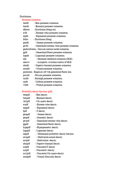
Distributions.Parameter estimation.betafit - Beta parameter estimation.binofit - Binomial parameter estimation.dfittool - Distribution fitting tool.evfit - Extreme value parameter estimation.expfit - Exponential parameter estimation.fitdist - Distribution fitting.gamfit - Gamma parameter estimation.gevfit - Generalized extreme value parameter estimation.gmdistribution - Gaussian mixture model estimation.gpfit - Generalized Pareto parameter estimation.lognfit - Lognormal parameter estimation.mle - Maximum likelihood estimation (MLE).mlecov - Asymptotic covariance matrix of MLE.nbinfit - Negative binomial parameter estimation.normfit - Normal parameter estimation.paretotails - Empirical cdf with generalized Pareto tails.poissfit - Poisson parameter estimation.raylfit - Rayleigh parameter estimation.unifit - Uniform parameter estimation.wblfit - Weibull parameter estimation.Probability density functions (pdf).betapdf - Beta density.binopdf - Binomial density.chi2pdf - Chi square density.evpdf - Extreme value density.exppdf - Exponential density.fpdf - F density.gampdf - Gamma density.geopdf - Geometric density.gevpdf - Generalized extreme value density.gppdf - Generalized Pareto density.hygepdf - Hypergeometric density.lognpdf - Lognormal density.mnpdf - Multinomial probability density function.mvnpdf - Multivariate normal density.mvtpdf - Multivariate t density.nbinpdf - Negative binomial density.ncfpdf - Noncentral F density.nctpdf - Noncentral t density.ncx2pdf - Noncentral Chi-square density.normpdf - Normal (Gaussian) density.pdf - Density function for a specified distribution.poisspdf - Poisson density.raylpdf - Rayleigh density.tpdf - T density.unidpdf - Discrete uniform density.unifpdf - Uniform density.wblpdf - Weibull density.Cumulative Distribution functions (cdf).betacdf - Beta cumulative distribution function.binocdf - Binomial cumulative distribution function.cdf - Specified cumulative distribution function.chi2cdf - Chi square cumulative distribution function.ecdf - Empirical cumulative distribution function (Kaplan-Meier estimate). evcdf - Extreme value cumulative distribution function.expcdf - Exponential cumulative distribution function.fcdf - F cumulative distribution function.gamcdf - Gamma cumulative distribution function.geocdf - Geometric cumulative distribution function.gevcdf - Generalized extreme value cumulative distribution function.gpcdf - Generalized Pareto cumulative distribution function.hygecdf - Hypergeometric cumulative distribution function.logncdf - Lognormal cumulative distribution function.mvncdf - Multivariate normal cumulative distribution function.mvtcdf - Multivariate t cumulative distribution function.nbincdf - Negative binomial cumulative distribution function.ncfcdf - Noncentral F cumulative distribution function.nctcdf - Noncentral t cumulative distribution function.ncx2cdf - Noncentral Chi-square cumulative distribution function.normcdf - Normal (Gaussian) cumulative distribution function.poisscdf - Poisson cumulative distribution function.raylcdf - Rayleigh cumulative distribution function.tcdf - T cumulative distribution function.unidcdf - Discrete uniform cumulative distribution function.unifcdf - Uniform cumulative distribution function.wblcdf - Weibull cumulative distribution function.Critical Values of Distribution functions.betainv - Beta inverse cumulative distribution function.binoinv - Binomial inverse cumulative distribution function.chi2inv - Chi square inverse cumulative distribution function.evinv - Extreme value inverse cumulative distribution function.expinv - Exponential inverse cumulative distribution function.finv - F inverse cumulative distribution function.gaminv - Gamma inverse cumulative distribution function.geoinv - Geometric inverse cumulative distribution function.gevinv - Generalized extreme value inverse cumulative distribution function. gpinv - Generalized Pareto inverse cumulative distribution function. hygeinv - Hypergeometric inverse cumulative distribution function.icdf - Specified inverse cumulative distribution function.logninv - Lognormal inverse cumulative distribution function.nbininv - Negative binomial inverse distribution function.ncfinv - Noncentral F inverse cumulative distribution function.nctinv - Noncentral t inverse cumulative distribution function.ncx2inv - Noncentral Chi-square inverse distribution function.norminv - Normal (Gaussian) inverse cumulative distribution function. poissinv - Poisson inverse cumulative distribution function.raylinv - Rayleigh inverse cumulative distribution function.tinv - T inverse cumulative distribution function.unidinv - Discrete uniform inverse cumulative distribution function.unifinv - Uniform inverse cumulative distribution function.wblinv - Weibull inverse cumulative distribution function.Random Number Generators.betarnd - Beta random numbers.binornd - Binomial random numbers.chi2rnd - Chi square random numbers.evrnd - Extreme value random numbers.exprnd - Exponential random numbers.frnd - F random numbers.gamrnd - Gamma random numbers.geornd - Geometric random numbers.gevrnd - Generalized extreme value random numbers.gprnd - Generalized Pareto inverse random numbers.hygernd - Hypergeometric random numbers.iwishrnd - Inverse Wishart random matrix.johnsrnd - Random numbers from the Johnson system of distributions. lognrnd - Lognormal random numbers.mhsample - Metropolis-Hastings algorithm.mnrnd - Multinomial random vectors.mvnrnd - Multivariate normal random vectors.mvtrnd - Multivariate t random vectors.nbinrnd - Negative binomial random numbers.ncfrnd - Noncentral F random numbers.nctrnd - Noncentral t random numbers.ncx2rnd - Noncentral Chi-square random numbers.normrnd - Normal (Gaussian) random numbers.pearsrnd - Random numbers from the Pearson system of distributions.poissrnd - Poisson random numbers.randg - Gamma random numbers (unit scale). random - Random numbers from specified distribution. randsample - Random sample from finite population. raylrnd - Rayleigh random numbers.slicesample - Slice sampling method.trnd - T random numbers.unidrnd - Discrete uniform random numbers.unifrnd - Uniform random numbers.wblrnd - Weibull random numbers.wishrnd - Wishart random matrix.Quasi-Random Number Generators.haltonset - Halton sequence point set. qrandstream - Quasi-random stream.sobolset - Sobol sequence point set.Statistics.betastat - Beta mean and variance.binostat - Binomial mean and variance.chi2stat - Chi square mean and variance.evstat - Extreme value mean and variance.expstat - Exponential mean and variance.fstat - F mean and variance.gamstat - Gamma mean and variance.geostat - Geometric mean and variance.gevstat - Generalized extreme value mean and variance. gpstat - Generalized Pareto inverse mean and variance. hygestat - Hypergeometric mean and variance.lognstat - Lognormal mean and variance.nbinstat - Negative binomial mean and variance. ncfstat - Noncentral F mean and variance.nctstat - Noncentral t mean and variance.ncx2stat - Noncentral Chi-square mean and variance. normstat - Normal (Gaussian) mean and variance. poisstat - Poisson mean and variance.raylstat - Rayleigh mean and variance.tstat - T mean and variance.unidstat - Discrete uniform mean and variance.unifstat - Uniform mean and variance.wblstat - Weibull mean and variance.Likelihood functions.betalike - Negative beta log-likelihood.evlike - Negative extreme value log-likelihood.explike - Negative exponential log-likelihood.gamlike - Negative gamma log-likelihood.gevlike - Generalized extreme value log-likelihood.gplike - Generalized Pareto inverse log-likelihood.lognlike - Negative lognormal log-likelihood.nbinlike - Negative binomial log-likelihood.normlike - Negative normal likelihood.wbllike - Negative Weibull log-likelihood.Probability distribution objects.ProbDistUnivKernel - Univariate kernel smoothing distributions. ProbDistUnivParam - Univariate parametric distributions.Descriptive Statistics.bootci - Bootstrap confidence intervals.bootstrp - Bootstrap statistics.corr - Linear or rank correlation coefficient.corrcoef - Linear correlation coefficient (in MATLAB toolbox).cov - Covariance (in MATLAB toolbox).crosstab - Cross tabulation.geomean - Geometric mean.grpstats - Summary statistics by group.harmmean - Harmonic mean.iqr - Interquartile range.jackknife - Jackknife statistics.kurtosis - Kurtosis.mad - Median Absolute Deviation.mean - Sample average (in MATLAB toolbox).median - 50th percentile of a sample (in MATLAB toolbox).mode - Mode, or most frequent value in a sample (in MATLAB toolbox). moment - Moments of a sample.nancov - Covariance matrix ignoring NaNs.nanmax - Maximum ignoring NaNs.nanmean - Mean ignoring NaNs.nanmedian - Median ignoring NaNs.nanmin - Minimum ignoring NaNs.nanstd - Standard deviation ignoring NaNs.nansum - Sum ignoring NaNs.nanvar - Variance ignoring NaNs.partialcorr - Linear or rank partial correlation coefficient.prctile - Percentiles.quantile - Quantiles.range - Range.skewness - Skewness.std - Standard deviation (in MATLAB toolbox).tabulate - Frequency table.trimmean - Trimmed mean.var - Variance (in MATLAB toolbox).Linear Models.addedvarplot - Created added-variable plot for stepwise regression.anova1 - One-way analysis of variance.anova2 - Two-way analysis of variance.anovan - n-way analysis of variance.aoctool - Interactive tool for analysis of covariance.dummyvar - Dummy-variable coding.friedman - Friedman's test (nonparametric two-way anova).glmfit - Generalized linear model fitting.glmval - Evaluate fitted values for generalized linear model.invpred - Inverse prediction for simple linear regression.kruskalwallis - Kruskal-Wallis test (nonparametric one-way anova).leverage - Regression diagnostic.lscov - Ordinary, weighted, or generalized least-squares (in MATLAB toolbox). lsqnonneg - Non-negative least-squares (in MATLAB toolbox).manova1 - One-way multivariate analysis of variance.manovacluster - Draw clusters of group means for manova1.mnrfit - Nominal or ordinal multinomial regression model fitting.mnrval - Predict values for nominal or ordinal multinomial regression. multcompare - Multiple comparisons of means and other estimates.mvregress - Multivariate regression with missing data.mvregresslike - Negative log-likelihood for multivariate regression.polyconf - Polynomial evaluation and confidence interval estimation.polyfit - Least-squares polynomial fitting (in MATLAB toolbox).polyval - Predicted values for polynomial functions (in MATLAB toolbox). rcoplot - Residuals case order plot.regress - Multiple linear regression using least squares.regstats - Regression diagnostics.ridge - Ridge regression.robustfit - Robust regression model fitting.rstool - Multidimensional response surface visualization (RSM).stepwise - Interactive tool for stepwise regression.stepwisefit - Non-interactive stepwise regression.x2fx - Factor settings matrix (x) to design matrix (fx).Nonlinear Models.coxphfit - Cox proportional hazards regression.nlinfit - Nonlinear least-squares data fitting.nlintool - Interactive graphical tool for prediction in nonlinear models. nlmefit - Nonlinear mixed-effects data fitting.nlpredci - Confidence intervals for prediction.nlparci - Confidence intervals for parameters.Design of Experiments (DOE).bbdesign - Box-Behnken design.candexch - D-optimal design (row exchange algorithm for candidate set). candgen - Candidates set for D-optimal design generation.ccdesign - Central composite design.cordexch - D-optimal design (coordinate exchange algorithm). daugment - Augment D-optimal design.dcovary - D-optimal design with fixed covariates.fracfactgen - Fractional factorial design generators.ff2n - Two-level full-factorial design.fracfact - Two-level fractional factorial design.fullfact - Mixed-level full-factorial design.hadamard - Hadamard matrices (orthogonal arrays) (in MATLAB toolbox). lhsdesign - Latin hypercube sampling design.lhsnorm - Latin hypercube multivariate normal sample.rowexch - D-optimal design (row exchange algorithm).Statistical Process Control (SPC).capability - Capability indices.capaplot - Capability plot.controlchart - Shewhart control chart.controlrules - Control rules (Western Electric or Nelson) for SPC data.gagerr - Gage repeatability and reproducibility (R&R) study.histfit - Histogram with superimposed normal density.normspec - Plot normal density between specification limits.runstest - Runs test for randomness.Multivariate Statistics.Cluster Analysis.cophenet - Cophenetic coefficient.cluster - Construct clusters from LINKAGE output.clusterdata - Construct clusters from data.dendrogram - Generate dendrogram plot.gmdistribution - Gaussian mixture model estimation.inconsistent - Inconsistent values of a cluster tree.kmeans - k-means clustering.linkage - Hierarchical cluster information.pdist - Pairwise distance between observations.silhouette - Silhouette plot of clustered data.squareform - Square matrix formatted distance.Classification.classify - Linear discriminant analysis.NaiveBayes - Naive Bayes classification.Dimension Reduction Techniques.factoran - Factor analysis.nnmf - Non-negative matrix factorization.pcacov - Principal components from covariance matrix. pcares - Residuals from principal components.princomp - Principal components analysis from raw data. rotatefactors - Rotation of FA or PCA loadings.Copulascopulacdf - Cumulative probability function for a copula. copulafit - Fit a parametric copula to data.copulaparam - Copula parameters as a function of rank correlation. copulapdf - Probability density function for a copula. copularnd - Random vectors from a copula.copulastat - Rank correlation for a copula.Plotting.andrewsplot - Andrews plot for multivariate data.biplot - Biplot of variable/factor coefficients and scores. interactionplot - Interaction plot for factor effects. maineffectsplot - Main effects plot for factor effects.glyphplot - Plot stars or Chernoff faces for multivariate data. gplotmatrix - Matrix of scatter plots grouped by a common variable. multivarichart - Multi-vari chart of factor effects. parallelcoords - Parallel coordinates plot for multivariate data.Other Multivariate Methods.barttest - Bartlett's test for dimensionality.canoncorr - Canonical correlation analysis.cmdscale - Classical multidimensional scaling.mahal - Mahalanobis distance.manova1 - One-way multivariate analysis of variance. mdscale - Metric and non-metric multidimensional scaling. mvregress - Multivariate regression with missing data. plsregress - Partial least squares regression.procrustes - Procrustes analysis.Decision Tree Techniques.classregtree - Classification and regression tree.TreeBagger - Ensemble of bagged decision trees. CompactTreeBagger - Lightweight ensemble of bagged decision trees.Hypothesis Tests.ansaribradley - Ansari-Bradley two-sample test for equal dispersions.dwtest - Durbin-Watson test for autocorrelation in linear regression. linhyptest - Linear hypothesis test on parameter estimates.ranksum - Wilcoxon rank sum test (independent samples).runstest - Runs test for randomness.sampsizepwr - Sample size and power calculation for hypothesis test. signrank - Wilcoxon sign rank test (paired samples).signtest - Sign test (paired samples).ttest - One sample t test.ttest2 - Two sample t test.vartest - One-sample test of variance.vartest2 - Two-sample F test for equal variances.vartestn - Test for equal variances across multiple groups.ztest - Z test.Distribution Testing.chi2gof - Chi-square goodness-of-fit test.jbtest - Jarque-Bera test of normality.kstest - Kolmogorov-Smirnov test for one sample.kstest2 - Kolmogorov-Smirnov test for two samples.lillietest - Lilliefors test of normality.Nonparametric Functions.friedman - Friedman's test (nonparametric two-way anova). kruskalwallis - Kruskal-Wallis test (nonparametric one-way anova). ksdensity - Kernel smoothing density estimation.ranksum - Wilcoxon rank sum test (independent samples).signrank - Wilcoxon sign rank test (paired samples).signtest - Sign test (paired samples).Hidden Markov Models.hmmdecode - Calculate HMM posterior state probabilities. hmmestimate - Estimate HMM parameters given state information. hmmgenerate - Generate random sequence for HMM.hmmtrain - Calculate maximum likelihood estimates for HMM parameters. hmmviterbi - Calculate most probable state path for HMM sequence.Model Assessment.confusionmat - Confusion matrix for classification algorithms.crossval - Loss estimate using cross-validation.cvpartition - Cross-validation partition.perfcurve - ROC and other performance measures for classification algorithms.Model Selection.sequentialfs - Sequential feature selection.stepwise - Interactive tool for stepwise regression.stepwisefit - Non-interactive stepwise regression.Statistical Plotting.andrewsplot - Andrews plot for multivariate data.biplot - Biplot of variable/factor coefficients and scores.boxplot - Boxplots of a data matrix (one per column).cdfplot - Plot of empirical cumulative distribution function.ecdf - Empirical cdf (Kaplan-Meier estimate).ecdfhist - Histogram calculated from empirical cdf.fsurfht - Interactive contour plot of a function.gline - Point, drag and click line drawing on figures.glyphplot - Plot stars or Chernoff faces for multivariate data.gname - Interactive point labeling in x-y plots.gplotmatrix - Matrix of scatter plots grouped by a common variable.gscatter - Scatter plot of two variables grouped by a third.hist - Histogram (in MATLAB toolbox).hist3 - Three-dimensional histogram of bivariate data.ksdensity - Kernel smoothing density estimation.lsline - Add least-square fit line to scatter plot.normplot - Normal probability plot.parallelcoords - Parallel coordinates plot for multivariate data.probplot - Probability plot.qqplot - Quantile-Quantile plot.refcurve - Reference polynomial curve.refline - Reference line.scatterhist - 2D scatter plot with marginal histograms.surfht - Interactive contour plot of a data grid.wblplot - Weibull probability plot.Data Objectsdataset - Create datasets from workspace variables or files.nominal - Create arrays of nominal data.ordinal - Create arrays of ordinal data.Statistics Demos.aoctool - Interactive tool for analysis of covariance.disttool - GUI tool for exploring probability distribution functions.polytool - Interactive graph for prediction of fitted polynomials. randtool - GUI tool for generating random numbers.rsmdemo - Reaction simulation (DOE, RSM, nonlinear curve fitting). robustdemo - Interactive tool to compare robust and least squares fits.File Based I/O.tblread - Read in data in tabular format.tblwrite - Write out data in tabular format to file.tdfread - Read in text and numeric data from tab-delimited file. caseread - Read in case names.casewrite - Write out case names to file.Utility Functions.cholcov - Cholesky-like decomposition for covariance matrix. combnk - Enumeration of all combinations of n objects k at a time. corrcov - Convert covariance matrix to correlation matrix.grp2idx - Convert grouping variable to indices and array of names. hougen - Prediction function for Hougen model (nonlinear example). statget - Get STATS options parameter value.statset - Set STATS options parameter value.tiedrank - Compute ranks of sample, adjusting for ties.zscore - Normalize matrix columns to mean 0, variance 1.Overloaded methods:xregusermod/statsxregunispline/statsxregnnet/statsxregmultilin/statsxregmodel/statsxreglinear/statsxreginterprbf/statsxregarx/stats。

Package‘glmmfields’October20,2023Type PackageTitle Generalized Linear Mixed Models with Robust Random Fields for Spatiotemporal ModelingVersion0.1.8Description Implements Bayesian spatial and spatiotemporalmodels that optionally allow for extreme spatial deviations throughtime.'glmmfields'uses a predictive process approach with randomfields implemented through a multivariate-t distribution instead ofthe usual multivariate normal.Sampling is conducted with'Stan'.References:Anderson and Ward(2019)<doi:10.1002/ecy.2403>. License GPL(>=3)URL https:///seananderson/glmmfieldsBugReports https:///seananderson/glmmfields/issues Depends methods,R(>=3.4.0),Rcpp(>=0.12.18)Imports assertthat,broom,broom.mixed,cluster,dplyr(>=0.8.0), forcats,ggplot2(>=2.2.0),loo(>=2.0.0),mvtnorm,nlme,RcppParallel(>=5.0.1),reshape2,rstan(>=2.26.0),rstantools(>=2.1.1),tibbleSuggests bayesplot,coda,knitr,parallel,rmarkdown,testthat,viridisLinkingTo BH(>=1.66.0),Rcpp(>=0.12.8),RcppEigen(>=0.3.3.3.0), RcppParallel(>=5.0.1),rstan(>=2.26.0),StanHeaders(>=2.26.0)VignetteBuilder knitrEncoding UTF-8RoxygenNote7.2.3SystemRequirements GNU makeNeedsCompilation yesBiarch true12glmmfields-package Author Sean C.Anderson[aut,cre],Eric J.Ward[aut],Trustees of Columbia University[cph]Maintainer Sean C.Anderson<********************>Repository CRANDate/Publication2023-10-2017:50:02UTCR topics documented:glmmfields-package (2)format_data (3)glmmfields (4)lognormal (7)loo.glmmfields (8)nbinom2 (8)plot.glmmfields (9)predict (10)sim_glmmfields (12)stan_pars (13)student_t (14)tidy (14)Index16 glmmfields-package The’glmmfields’package.DescriptionImplements Bayesian spatial and spatiotemporal models that optionally allow for extreme spatial deviations through time.’glmmfields’uses a predictive process approach with randomfields im-plemented through a multivariate-t distribution instead of the usual multivariate normal.Sampling is conducted with’Stan’.ReferencesStan Development Team(2018).RStan:the R interface to Stan.R package version2.18.2.format_data3 format_data Format data forfitting a glmmfields modelDescriptionFormat data forfitting a glmmfields modelUsageformat_data(data,y,X,time,lon="lon",lat="lat",station=NULL,nknots=25L,covariance=c("squared-exponential","exponential","matern"),fixed_intercept=FALSE,cluster=c("pam","kmeans"))Argumentsdata A data frame to be formattedy A numeric vector of the responseX A matrix of the predictorstime A character object giving the name of the time columnlon A character object giving the name of the longitude columnlat A character object giving the name of the latitude columnstation A numeric vector giving the integer ID of the stationnknots The number of knotscovariance The type of covariance functionfixed_interceptShould the intercept befixed?cluster The type of clustering algorithm used to determine the not locations."pam"= pam.kmeans is faster for large datasets.glmmfields Fit a spatiotemporal randomfields GLMMDescriptionFit a spatiotemporal randomfields model that optionally uses the MVT distribution instead of a MVN distribution to allow for spatial extremes through time.It is also possible tofit a spatial randomfields model without a time component.Usageglmmfields(formula,data,lon,lat,time=NULL,nknots=15L,prior_gp_theta=half_t(3,0,5),prior_gp_sigma=half_t(3,0,5),prior_sigma=half_t(3,0,5),prior_rw_sigma=half_t(3,0,5),prior_intercept=student_t(3,0,10),prior_beta=student_t(3,0,3),prior_phi=student_t(1000,0,0.5),fixed_df_value=1000,fixed_phi_value=0,estimate_df=FALSE,estimate_ar=FALSE,family=gaussian(link="identity"),binomial_N=NULL,covariance=c("squared-exponential","exponential","matern"),matern_kappa=0.5,algorithm=c("sampling","meanfield"),year_re=FALSE,nb_lower_truncation=0,control=list(adapt_delta=0.9),save_log_lik=FALSE,df_lower_bound=2,cluster=c("pam","kmeans"),offset=NULL,...)Argumentsformula The model formula.data A data frame.lon A character object giving the name of the longitude column.lat A character object giving the name of the latitude column.time A character object giving the name of the time column.Leave as NULL tofit a spatial GLMM without a time element.nknots The number of knots to use in the predictive process model.Smaller values will be faster but may not adequately represent the shape of the spatial pattern. prior_gp_theta The prior on the Gaussian Process scale parameter.Must be declared with half_t().Here,and throughout,priors that are normal or half-normal can beimplemented by setting thefirst parameter in the half-t or student-t distributionto a large value.E.g.something greater than100.prior_gp_sigma The prior on the Gaussian Process eta parameter.Must be declared with half_t(). prior_sigma The prior on the observation process scale parameter.Must be declared with half_t().This acts as a substitute for the scale parameter in whatever obser-vation distribution is being used.E.g.the CV for the Gamma or the dispersionparameter for the negative binomial.prior_rw_sigma The prior on the standard deviation parameter of the random walk process(if specified).Must be declared with half_t().prior_interceptThe prior on the intercept parameter.Must be declared with student_t(). prior_beta The prior on the slope parameters(if any).Must be declared with student_t(). prior_phi The prior on the AR parameter.Must be declared with student_t().fixed_df_value Thefixed value for the student-t degrees of freedom parameter if the degrees of freedom parameter isfixed in the MVT.If the degrees of freedom parameteris estimated then this argument is ignored.Must be1or greater.Very largevalues(e.g.the default value)approximate the normal distribution.If the valueis>=1000then a true MVN distribution will befit.fixed_phi_valueThefixed value for temporal autoregressive parameter,between randomfieldsat time(t)and time(t-1).If the phi parameter is estimated then this argument isignored.estimate_df Logical:should the degrees of freedom parameter be estimated?estimate_ar Logical:should the AR(autoregressive)parameter be estimated?Here,this refers to a autoregressive process in the evolution of the spatialfield throughtime.family Family object describing the observation model.Note that only one link is implemented for each distribution.Gamma,negative binomial(specified vianbinom2()as nbinom2(link="log"),and Poisson must have a log link.Bi-nomial must have a logit link.Also implemented is the lognormal(specifiedvia lognormal()as lognormal(link="log").Besides the negative binomialand lognormal,other families are specified as shown in family.binomial_N A character object giving the optional name of the column containing Binomial sample size.Leave as NULL tofit a spatial GLMM with sample sizes(N)=1,equivalent to bernoulli model.covariance The covariance function of the Gaussian Process.One of"squared-exponential", "exponential",or"matern".matern_kappa Optional parameter for the Matern covariance function.Optional values are1.5 or2.5.Values of0.5are equivalent to exponential.algorithm Character object describing whether the model should befit with full NUTS MCMC or via the variational inference mean-field approach.See rstan::vb().Note that the variational inference approach should not be trusted forfinal infer-ence and is much more likely to give incorrect inference than MCMC.year_re Logical:estimate a random walk for the time variable?If TRUE,then nofixed effects(B coefficients)will be estimated.In this case,prior_intercept willbe used as the prior for the initial value in time.nb_lower_truncationFor NB2only:lower truncation value. E.g.0for no truncation,1for1andall values above.Note that estimation is likely to be considerably slower withlower truncation because the sampling is not vectorized.Also note that thelog likelihood values returned for estimating quantities like LOOIC will not becorrect if lower truncation is implemented.control List to pass to rstan::sampling().For example,increase adapt_delta if there are warnings about divergent transitions:control=list(adapt_delta=0.99).By default,glmmfields sets adapt_delta=0.9.save_log_lik Logical:should the log likelihood for each data point be saved so that informa-tion criteria such as LOOIC or W AIC can be calculated?Defaults to FALSE sothat the size of model objects is smaller.df_lower_bound The lower bound on the degrees of freedom parameter.Values that are too low,e.g.below2or3,it might affect chain convergence.Defaults to2.cluster The type of clustering algorithm used to determine the knot locations."pam"= cluster::pam().The"kmeans"algorithm will be faster on larger datasets.offset An optional offset vector....Any other arguments to pass to rstan::sampling().DetailsNote that there is no guarantee that the default priors are reasonable for your data.Also,there is no guarantee the default priors will remain the same in future versions.Therefore it is important that you specify any priors that are used in your model,even if they replicate the defaults in the package.It is particularly important that you consider that prior on gp_theta since it depends on the distance between your location points.You may need to scale your coordinate units so they are on a ballpark range of1-10by,say,dividing the coordinates(say in UTMs)by several order of magnitude.Examples#Spatiotemporal example:set.seed(1)s<-sim_glmmfields(n_draws=12,n_knots=12,gp_theta=1.5,gp_sigma=0.2,sd_obs=0.2)lognormal7 print(s$plot)#options(mc.cores=parallel::detectCores())#for parallel processing#should use4or more chains for real model fitsm<-glmmfields(y~0,time="time",lat="lat",lon="lon",data=s$dat,nknots=12,iter=1000,chains=2,seed=1)#Spatial example(with covariates)from the vignette and customizing#some priors:set.seed(1)N<-100#number of data pointstemperature<-rnorm(N,0,1)#simulated temperature dataX<-cbind(1,temperature)#design matrixs<-sim_glmmfields(n_draws=1,gp_theta=1.2,n_data_points=N,gp_sigma=0.3,sd_obs=0.1,n_knots=12,obs_error="gamma",covariance="squared-exponential",X=X,B=c(0.5,0.2))#B represents our intercept and sloped<-s$datd$temperature<-temperaturelibrary(ggplot2)ggplot(s$dat,aes(lon,lat,colour=y))+viridis::scale_colour_viridis()+geom_point(size=3)m_spatial<-glmmfields(y~temperature,data=d,family=Gamma(link="log"),lat="lat",lon="lon",nknots=12,iter=2000,chains=2,prior_beta=student_t(100,0,1),prior_intercept=student_t(100,0,5),control=list(adapt_delta=0.95))lognormal Lognormal familyDescriptionLognormal familyUsagelognormal(link="log")Argumentslink The link(must be log)Exampleslognormal()8nbinom2 loo.glmmfields Return LOO information criteriaDescriptionExtract the LOOIC(leave-one-out information criterion)using loo::loo().Usage##S3method for class glmmfieldsloo(x,...)Argumentsx Output from glmmfields().Must befit with save_log_lik=TRUE,which is not the default....Arguments for loo::relative_eff()and loo::loo.array().Examplesset.seed(1)s<-sim_glmmfields(n_draws=12,n_knots=12,gp_theta=1.5,gp_sigma=0.2,sd_obs=0.2)#options(mc.cores=parallel::detectCores())#for parallel processing#save_log_lik defaults to FALSE to save space but is needed for loo():m<-glmmfields(y~0,time="time",lat="lat",lon="lon",data=s$dat,nknots=12,iter=1000,chains=4,seed=1,save_log_lik=TRUE)loo(m)nbinom2Negative binomial familyDescriptionThis is the NB2parameterization where the variance scales quadratically with the mean.Usagenbinom2(link="log")plot.glmmfields9Argumentslink The link(must be log)Examplesnbinom2()plot.glmmfields Plot predictions from an glmmfields modelDescriptionPlot predictions from an glmmfields modelUsage##S3method for class glmmfieldsplot(x,type=c("prediction","spatial-residual","residual-vs-fitted"),link=TRUE,...)Argumentsx An object returned by glmmfieldstype Type of plotlink Logical:should the plots be made on the link scale or on the natural scale?...Other arguments passed to predict.glmmfieldsExamples#Spatiotemporal example:set.seed(1)s<-sim_glmmfields(n_draws=12,n_knots=12,gp_theta=1.5,gp_sigma=0.2,sd_obs=0.1)#options(mc.cores=parallel::detectCores())#for parallel processingm<-glmmfields(y~0,time="time",lat="lat",lon="lon",data=s$dat,nknots=12,iter=600,chains=1)x<-plot(m,type="prediction")xx+ggplot2::scale_color_gradient2()plot(m,type="spatial-residual")plot(m,type="residual-vs-fitted")10predict predict Predict from a glmmfields modelDescriptionThese functions extract posterior draws or credible intervals.The helper functions are named to match those in the rstanarm package and call the function predict()with appropriate argument values.Usage##S3method for class glmmfieldspredictive_interval(object,...)##S3method for class glmmfieldsposterior_linpred(object,...)##S3method for class glmmfieldsposterior_predict(object,...)##S3method for class glmmfieldspredict(object,newdata=NULL,estimate_method=c("median","mean"),conf_level=0.95,interval=c("confidence","prediction"),type=c("link","response"),return_mcmc=FALSE,offset=NULL,iter="all",...)Argumentsobject An object returned by glmmfields()....Ignored currentlynewdata Optionally,a data frame to predict onestimate_methodMethod for computing point estimate("mean"or"median") conf_level Probability level for the credible intervals.interval Type of interval calculation.Same as for stats::predict.lm().type Whether the predictions are returned on"link"scale or"response"scale(Same as for stats::predict.glm()).predict11return_mcmc Logical.Should the full MCMC draws be returned for the predictions?offset Optional offset vector to be used in prediction.iter Number of MCMC iterations to draw.Defaults to all.Exampleslibrary(ggplot2)#simulate:set.seed(1)s<-sim_glmmfields(n_draws=12,n_knots=12,gp_theta=2.5,gp_sigma=0.2,sd_obs=0.1)#fit:#options(mc.cores=parallel::detectCores())#for parallel processingm<-glmmfields(y~0,data=s$dat,time="time",lat="lat",lon="lon",nknots=12,iter=800,chains=1)#Predictions:#Link scale credible intervals:p<-predict(m,type="link",interval="confidence")head(p)#Prediction intervals on new observations(include observation error):p<-predictive_interval(m)head(p)#Posterior prediction draws:p<-posterior_predict(m,iter=100)dim(p)#rows are iterations and columns are data elements#Draws from the linear predictor(not in link space):p<-posterior_linpred(m,iter=100)dim(p)#rows are iterations and columns are data elements#Use the tidy method to extract parameter estimates as a data frame:head(tidy(m,conf.int=TRUE,conf.method="HPDinterval"))#Make predictions on a fine-scale spatial grid:pred_grid<-expand.grid(lat=seq(min(s$dat$lat),max(s$dat$lat),length.out=25),lon=seq(min(s$dat$lon),max(s$dat$lon),length.out=25),time=unique(s$dat$time))pred_grid$prediction<-predict(m,newdata=pred_grid,type="response",iter=100,12sim_glmmfields estimate_method="median",offset=rep(0,nrow(pred_grid)))$estimateggplot(pred_grid,aes(lon,lat,fill=prediction))+facet_wrap(~time)+geom_raster()+scale_fill_gradient2()sim_glmmfields Simulate a randomfield with a MVT distributionDescriptionSimulate a randomfield with a MVT distributionUsagesim_glmmfields(n_knots=15,n_draws=10,gp_theta=0.5,gp_sigma=0.2,mvt=TRUE,df=1e+06,seed=NULL,n_data_points=100,sd_obs=0.1,covariance=c("squared-exponential","exponential","matern"),matern_kappa=0.5,obs_error=c("normal","gamma","poisson","nb2","binomial","lognormal"),B=c(0),phi=0,X=rep(1,n_draws*n_data_points),g=data.frame(lon=runif(n_data_points,0,10),lat=runif(n_data_points,0,10)) )Argumentsn_knots The number of knotsn_draws The number of draws(for example,the number of years)gp_theta The Gaussian Process scale parametergp_sigma The Gaussian Process variance parametermvt Logical:MVT?(vs.MVN)df The degrees of freedom parameter for the MVT distributionseed The random seed valuestan_pars13n_data_points The number of data points per drawsd_obs The observation process scale parametercovariance The covariance function of the Gaussian process("squared-exponential","expo-nential","matern")matern_kappa The optional matern parameter.Can be1.5or2.5.Values of0.5equivalent to exponential model.obs_error The observation error distributionB A vector of parameters.Thefirst element is the interceptphi The auto regressive parameter on the mean of the randomfield knotsX The model matrixg Grid of pointsExampless<-sim_glmmfields(n_draws=12,n_knots=12,gp_theta=1.5,gp_sigma=0.2,sd_obs=0.2)names(s)stan_pars Return a vector of parametersDescriptionReturn a vector of parametersUsagestan_pars(obs_error,estimate_df=TRUE,est_temporalRE=FALSE,estimate_ar=FALSE,fixed_intercept=FALSE,save_log_lik=FALSE)Argumentsobs_error The observation error distributionestimate_df Logical indicating whether the degrees of freedom parameter should be esti-matedest_temporalRE Logical:estimate a random walk for the time variable?estimate_ar Logical indicating whether the ar parameter should be estimated14tidy fixed_interceptShould the intercept befixed?save_log_lik Logical:should the log likelihood for each data point be saved so that informa-tion criteria such as LOOIC or W AIC can be calculated?Defaults to FALSE sothat the size of model objects is smaller.student_t Student-t and half-t priorsDescriptionStudent-t and half-t priors.Note that this can be used to represent an effectively normal distribution prior by setting thefirst argument(the degrees of freedom parameter)to a large value(roughly50 or above).Usagestudent_t(df=3,location=0,scale=1)half_t(df=3,location=0,scale=1)Argumentsdf Degrees of freedom parameterlocation Location parameterscale Scale parameterExamplesstudent_t(3,0,1)half_t(3,0,1)tidy Tidy model outputDescriptionTidy model outputUsagetidy(x,...)##S3method for class glmmfieldstidy(x,...)tidy15Argumentsx Output from glmmfields()...Other argumentsIndexcluster::pam(),6family,5format_data,3glmmfields,4,9glmmfields(),8,10,15glmmfields-package,2half_t(student_t),14half_t(),5lognormal,7lognormal(),5loo(loo.glmmfields),8loo.glmmfields,8loo::loo(),8loo::loo.array(),8loo::relative_eff(),8nbinom2,8nbinom2(),5pam,3plot.glmmfields,9posterior_linpred(predict),10posterior_predict(predict),10predict,10predict.glmmfields,9predictive_interval(predict),10 rstan::sampling(),6rstan::vb(),6sim_glmmfields,12stan_pars,13stats::predict.glm(),10stats::predict.lm(),10student_t,14student_t(),5tidy,1416。

泊松自回归模型matlab全文共四篇示例，供读者参考第一篇示例：泊松自回归模型（Poisson Autoregressive Model）是一种用于计数数据分析的统计模型，常用于分析时间序列数据中的计数变量。

该模型主要用于描述某一时间点上计数变量的取值与之前时间点计数变量的取值之间的关系，并且考虑到计数数据的离散性和非负性。

在实际应用中，泊松自回归模型通常被应用于疾病发生率、环境污染、人口增长等领域的数据分析中，用来建立计数变量和时间相关性的模型，预测未来的计数值。

在本文中，我们将介绍如何使用Matlab软件来实现泊松自回归模型。

一、泊松分布简介泊松分布是概率论中常用的一种分布，用于描述单位时间或单位面积内随机事件的次数。

泊松分布的概率质量函数为：P(X=k) = (λ^k * e^(-λ)) / k!λ是随机事件在单位时间或单位面积上的平均发生率，k是随机事件发生的次数。

二、泊松自回归模型的定义泊松自回归模型是一种基于泊松分布的时间序列模型，用于描述计数变量在时间上的自回归关系。

泊松自回归模型的一般形式为：Y(t) = α + β1 * Y(t-1) + β2 * Y(t-2) + ... + βp * Y(t-p) + ε(t)Y(t)是在时间t上的计数变量的取值，α是截距，β1，β2，...，βp 是模型的回归系数，p是自回归阶数，ε(t)是误差项。

三、使用Matlab实现泊松自回归模型在Matlab中，可以使用泊松回归函数fitglm()来实现泊松自回归模型的拟合。

以下是一个简单的示例代码：```matlab% 生成模拟数据t = 1:100;Y = poissrnd(5,100,1);% 构建泊松自回归模型mdl = fitglm(t,Y,'poisson','Distribution','poisson');% 查看模型参数disp(mdl)```在上述代码中，首先生成了一个包含100个计数变量的模拟数据Y，然后使用fitglm()函数来拟合泊松自回归模型，指定分布类型为poisson。

R语言常用函数整理提示：碰到不懂的函数可以输入“？函数名”，前提条件是需要先安装包，使用命令“istall.packages(“包名”) 或菜单安装。

再载入包，除了几个基本包外，其他的包需要用“library(包名)”载入。

常用计量函数函数用途所在包线性回归及放宽条件lm 做线性回归statssummary() 返回回顾系数t、F检验等statsstatsglm 广义线性回归（probit logit passion回归以及WLS估计等）maxLik 极大似然估计（线性和非线性）maxLikpredict 求回归预测（对绝对部分模型都适用）statscoef 求回归结果系数statscor 求变量间person相关系数和spearman秩相关系数statsresid 返回回归残差statsfitted 返回拟合值statsscale 对数据进行标准化statslm.ridge 岭回归MASSplsr 偏最小二乘法plspcr 主成分回归plsbptest Breusch-Pagan异方差检验lmtest bartlett.test 做变量间方差齐性检验statsdwtest 做DW检验lmtestAIC 返回模型的AIC值statsvar.test 非参数方差齐性检验statsvif 求方差膨胀因子carapropos(“test”) 返回统计常用检验statsconfint() 计算回归模型参数的置信区间stats非线性优化和非线性回归optimize 做一元非线性优化statsoptim 做多元非线性优化stats constrOptim 约束下的非线性优化statsnls 非线性（加权）最小二乘估计statsmaxLik 非线性极大似然估计maxLiklogLik 求回归模型对数似然值statsexpand.grid 求格点statsnls2 类似于nls,但增加了brute-force算法nls2selfstart 生成自动初始值函数stats时间序列常用函数 时间序列描述统计exp() 求指数stats log() log()求自然对数，log10()求常对数，log2(),以2为底对数stats mean() 求向量均值 stats var() 求向量方差 stats sd() 求向量标准差 stats skewness 求向量偏度 e1071 kurtosis 求向量峰度e1071FinTS.stats 求时间序列描述统计量（包括均值、标准差、偏度、峰度等） FinTS t.test 检验时间序列均值是否为零（实际上可作单、双样本检验） statsARMA 相关函数ts 转换为时间序列格式 stats ts.plot 作时序图 stats diff.ts时序差分statsgetInitial 从自动生成初始值函数提取初始值 stats动态经济模型ts 把数据转换成时间序列格式 stats ts .union 合并(bind)时间序列数据 stats lag 对时间序列格式数据滞后 stats grangertest 葛兰杰因果关系检验lmtest 联立方程组systemfit 做联立方程2SLS 、3SLS 、SUR 估计等 systemfit cbind 对数据按列合并 base rbind 对数据按行合并base 离散因变量glmfamily=binomial(link=”probit”) 两元probit 模型 family=binomial(link=”logit”)两元logit 模型 family=passion 泊松回归 stats mlogit 多元logit 模型 mlogit polr 有序多元因变量模型 MASS(VR) stepAIC 利用AIC 准则做逐步回归 MASS tobit做tobit 模型AER面板数据分析plm 做面板数据固定效应、随机效应（包括个体、时间及其两者效应） plm phtest 面板数据Hausman 检验 plm pvcm 面板数据变系数估计 plmas.Date 把非时间向量转为时间向量 stats acf 求自相关函数和作偏自相关函数图 stats pacf 求偏自相关函数和作偏自相关函数图 stats Box.test 作序列自相关B-P 和L-B 检验stats ar 求自回归模型（包括ar.ols,ar.mle,ar.yw,ar.burg ） stats arima 求ARMA 、ARIMA 模型stats ARIMA 引用arima 函数，并增加了残差自相关L-B 检验 FinTS arma 使用条件最小二乘法估计，可任意设定滞后阶数(lag) tseries predict 作预测stats 等 tsdiag 时间序列诊断检验 stats adf.test ADF 检验tseries urdfTest ADF 检验(推荐使用) fUnitRoots kpss.test KPSS 平稳性检验 tseries pp.test Phillips-Perron 单位根检验 tseries Arima.sim 模拟生成给定ARIMA 模型的数据 stats FitAR 估计AR 模型及特定阶的AR 模型 FitAR自回归条件异方差相关函数garch GARCHtseriesgarchOxFit该函数求GARCH 相关模型非常方便， 求GARCH ，IGARCH,EGARCH,GARCH-M, T-GARCH 等 引用OX 软件的G@ARCH 。

numnpy中lognormal的概率密度分布函数-回复首先，我们来讨论一下NumPy中的lognormal分布。

lognormal分布是一种连续概率分布，它的概率密度函数具有以下形式：f(x, s) = (1 / (s * x * sqrt(2 * pi))) * exp(-1 * (log(x) - m)^2 / (2 * s^2))其中，m是对数平均值，s是对数标准差。

该概率密度函数表示了随机变量的对数服从正态分布的概率。

那么，我们如何使用NumPy来生成lognormal分布的概率密度函数呢？第一步是导入NumPy库：import numpy as np接下来，我们可以使用np.random.lognormal()函数来生成lognormal 分布的随机样本。

该函数的参数包括对数平均值m、对数标准差s以及样本个数size。

例如，生成1000个符合lognormal分布的随机样本，其中对数平均值为0，对数标准差为1：samples = np.random.lognormal(0, 1, 1000)然后，我们可以使用np.histogram()函数来计算概率密度函数的直方图。

该函数的第一个参数是随机样本，第二个参数是直方图的箱数。

hist, bin_edges = np.histogram(samples, bins=50, density=True)注意，我们将density参数设置为True，以计算概率密度函数的直方图。

现在，我们可以计算每个箱的中心值，作为概率密度函数的x轴坐标：bin_centers = (bin_edges[:-1] + bin_edges[1:]) / 2接下来，我们可以使用matplotlib库来绘制lognormal分布的概率密度函数图形。

首先，我们需要导入matplotlib库：import matplotlib.pyplot as plt然后，使用plt.plot()函数绘制概率密度函数的图形：plt.plot(bin_centers, hist)最后，我们可以使用plt.xlabel()和plt.ylabel()函数来为x轴和y轴添加标签，以及使用plt.title()函数来添加标题。