
统计学CH14 英文版
- 格式:ppt
- 大小:1.24 MB
- 文档页数:91
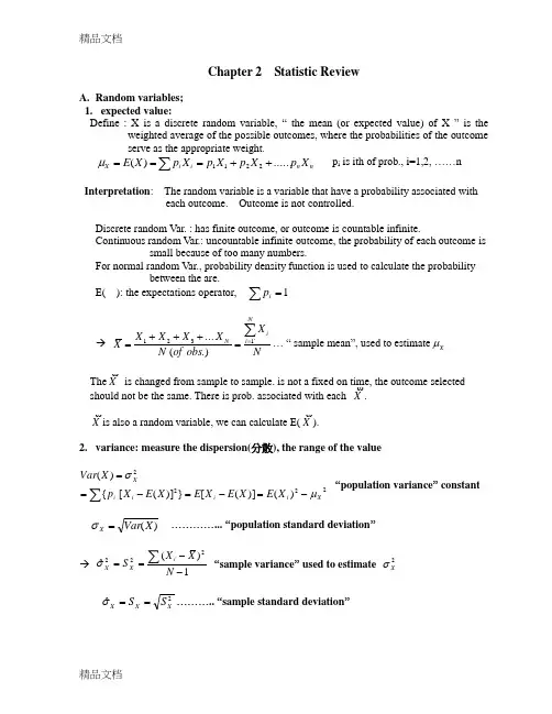
Chapter 2 Statistic ReviewA. Random variables; 1. expected value:Define : X is a discrete random variable, “ the mean (or expected value) of X ” is theweighted average of the possible outcomes, where the probabilities of the outcome serve as the appropriate weight.∑++===n n i i X X p X p X p X p X E ......)(2211μ p i is ith of prob., i=1,2, ……nInterpretation : The random variable is a variable that have a probability associated witheach outcome. Outcome is not controlled. Discrete random Var. : has finite outcome, or outcome is countable infinite.Continuous random Var.: uncountable infinite outcome, the probability of each outcome issmall because of too many numbers.For normal random Var., probability density function is used to calculate the probabilitybetween the are.E( ): the expectations operator, ∑=1i p→ NXobs of N X X X X X Ni iN∑==+++=`1321.)(....… “ sample mean ”, used to estimate X μThe X ϖis changed from sample to sample. is not a fixed on time, the outcome selected should not be the same. There is prob. associated with each X ϖ. X ϖis also a random variable, we can calculate E(X ϖ).2. variance: measure the dispersion(分散), the range of the value∑-=-=-==2222)()]([})]([{)(Xi i i i XX E X E X E X E X p X Var μσ “population variance ” constant)(X Var X =σ …………... “population standard deviation ”→ 1)(ˆ222--==∑N X X S iX X σ“sample variance ” used to estimate 2X σ2ˆX X X S S ==σ……….. “sample standard deviation ”3. joint distribution: (linear relation of X and Y bi-variance random variance.))])([(),(Y X Y X E Y X Cov μμ--=Covariance, measuring the linear relationship between X and Y.),(Y X Cov , depends on the units of X and Y; different unit-> different),(Y X Cov >0: the best-fitting line has a positive slope, positive relationship between X and Y . ),(Y X Cov <0: the best-fitting line has a negative slope, negative relationship between X and Y . ),(Y X Cov =0: there is no linear relationship between X and Y , but may be have nonlinearrelationship.YX XY Y X σσρ),cov(=“population correlation coefficient ” is scale free.XY ρ>0, a positive correction, XY ρ<0, a negative correction XY ρ=0, no linear relationship between X and Y11-≥≥XY ρ, XY ρ=1: regression line is a straight line with positive slope, XY ρ=-1: regressionline is a straight line with negative slope.1))((),(ˆ1---=∑=N Y Y X XY X vCo Ni i i,YX XYS S Y X ),(v ˆco =γ=221)()())((∑∑∑----=Y YX X Y Y X XiiNi i i“sample correlation coefficient ”)int (,1,1)(,1)(11prob jo pY p X p ijN i N j ij===∑∑∑∑==E(X) =0.263×1+0.403×2+0.334×3=2.071 Var(X) =4.881-(2.071)2=0.591959 E(Y) =0.298×6+0.385×5+0317×4=4.981 Var(Y)= 25.425-(4.981)2=0.614639Cov(X,Y)=)()(Y E X E Y X p ijj i j i -∑∑=10.001-2.071×4.981= -0.3174. formulaE(b)=b , Var(b)=0;E(aX)=aE(X), Var(aX)=a 2 Var(X ); E(aX+b)=aE(X)+b, Var(aX+b)= a 2 Var(X ))()]([)]}([{])([)]()[()(2222222X Var a X E X E a X E X a E b X aE b ax E b aX E b aX E b aX Var =-=-=+-+=+-+=+ΘE(X+Y)=E(X)+E(Y), Var(X+Y)=Var(X)+Var(Y)+2Cov(X, Y)\),(2)()()]}()][([2)]([)]({[)]}([)]({[)]()([)]()[()(22222Y X Cov Y Var X Var Y E Y X E X Y E Y X E X E Y E Y X E X E Y E X E Y X E Y X E Y X E Y X Var ++=----+-=-+-=--+=+-+=+Θ If X and Y is independent (linear uncorrelated), than E(X+Y)=E(X)+E(Y) → Cov(X,Y)=0, XY ρ=0, → Var(X+Y)=Var(X)+Var(Y))(][)]()()()([)]()][([),(=-=-=+--=+--=--=Y X Y X Y X Y X Y X XY E X Y XY E Y E X E Y XE X XE XY E Y E Y X E X E Y X Cov μμμμμμμμμμΘ,0),(=Y X Cov can ’t define the X and Y are independent. 2))(()(X E X X E ≠• X is not independent of itself.B. (probability) distributions:1. the normal distribution:),(`~2X X N X σμ2. the standard normal distribution:)1,0(~,N Z X Z XXσμ-=3. the Chi-square distribution:∑=+++==Ni N i NZ Z Z Z 12222122Λχ Z i : N independently normal distribution random variables with 0 mean and variance 1. → As N gets larger, the χ2 distribution because an approximation of normal distribution. the rang of χ2 : 0 → ∞ 4. the t distribution:If (1) Z is normal distribution with mean 0 and variance 1, (2) χ2 is distribution as Chi-square with N degrees of freedom, (3) Z and χ2 are independent Thenn nt NZ~2χ→As N gets large, the t distribution will tend to approximately be normal distribution. 5. the F distribution:if X and Y are independent and distribution as Chi-square will N1 and N2 degrees of freedom, respectively thus21,21~N N F N YN Xassume Xi ’s are independent each other,),(~2NX XX σμ regardless of the distribution of XE(X)=)(1)(1][21N i iX X X E NX E N NX E +++==∑∑Λ =X X X X X NN X X N μμμ=•=+++)(1Λ N N N X N X NX X X i i X22222)(1)var(1)1var()var(σσσ=•====∑∑22121)]()[()var(N N i X X X E X X X E X +++-+++=∑ΛΛΘ =22211)]}([)([)]({[N N X E X X E X X E X E -++-+-Λ =∑∑--+-)]()][([2)]([2j j i i i i X E X X E X E X E X =)var()var()var()var(21N i X X X X +++=∑Λ=2222X X X X N σσσσ=+++Λ If ),(~2XX N X σμ, then i.i.d. (independent with other variables, identically distributed over time) If ),(~2XX N X σμ, then ),(~2NN X XX σμ* Central limit theorem:If ),(~2XX X σμ (at any distribution), then ),(~2NN X XX σμ as N(sample size) increase.1)(ˆ2--==∑N X XS iX σ, what is the distribution of NS X 0μ- ?C. hypothesis testing:ex. H 0: μ=100… null hypothesis, H 1: μ≠100 …alternative hypothesis α=0.05 … level of significanceto get the value of X , the test statistic, NX Z 2100σ-=if σ2 is know.To check the critical value, Zc ( whether or not to accept H 0)If accept H 0:“we can not reject H 0 at 95% confidence level based on the data we have ”If reject H 0:“we can reject H 0 at 5% level of confidence.”Type I error: reject H 0 when H 0 is true, the probability of making type I error is α.Type II error: accept H 0 when H 0 is false, the probability of making type II error is difficult to determine.When the confidence interval increase, then the type I error will reduce and type II error will increase.※ 22000)1()1()()(σσμμμ---=-=-N S N NX S NX NS X Θ(1) if ),(~2XX N X σμ, then ),(~2NN X XX σμ, the numerator(分子) (NS X 0μ-) is the standardnormal variable Z, and22)1(σS N - is 21-N χ(21222222)()1()(11-=-=-⇒--=∑∑N i i X X S N X X N S χσσσσ)1210~)1(~----∴N N t N ZNS X χμ, if numerator and denominator(分母) are independent.(2) if ),(~2XX N X σμ, the we will appeal to the central limit theorem.D. point and interval estimate:1. point estimate: ex X =40 , but we don ’t know whether the true value approximates it ornot.2. interval estimate:NZ X Xσα2±, α=0.05 , if X σ is know.NS t X Xt 1,2-±α,α=0.05 , if X σ is unknown and N is small (<31).95% interval will include the true value.E. properties of estimator: unbiasedness, efficiency, consistency1. unbiasedness:βˆ is an unbiased estimator of β, if E(βˆ) =β(true value) → ex. X is an unbiased estimator of X μ;ex. 2X S is an unbiased estimator of 2X σ]})()([11{]1)([)(2222∑∑----=--=X X X N X N E N X X E SE μμ =222)(11X X X NN N N σσσ=-- ∑∑∑----+-=---=-)])((2)()[()]()[()(2222X X X X X X X X X X X X X X μμμμμμΘ =∑∑----+-)()(2)()(22X X X X X X X N X μμμμ =222)(2)()(X X X X N X N X μμμ---+-∑ =22)()(X X X N X μμ---∑→ bias= E(βˆ) -β2. efficiency:define: (a) minimum mean square error,MSE(βˆ)=E(βˆ-β)2 =[bias(βˆ)]2+Var(βˆ).Pove : 22]})([)](ˆ{[)ˆ(ββββββ-+-=-E E E E =]})([)](ˆ{[2])([)](ˆ[22ββββββββ--+-+-E E E E E E =)}ˆ()]ˆ([ˆ)ˆ(ˆ{2)]ˆ([)ˆvar(22βββββββββE E E E bias +--++ =0)]ˆ([)ˆvar(2++ββbias → we check X , it is mostly around μ.→ when bias(βˆ)=0, then MSE(βˆ)=Var(βˆ) → If we have an unbiased estimator with large dispersion of true value (ie. High var.) and abiased estimator with low var. we might prefer biased estimator than unbiased estimator to maximize the precision of prediction.Def. (b) If for a given sample size, (1) βˆis unbiased, (2) Var(βˆ))~var(β≤, when β~ is any other unbiased estimator of β. Then βˆ is an efficient estimator of β. Cramer-Rao lower bounds: gives a lower limit for the variance of any unbiased estimator.EX. The lower var(X )=N 2σ ; the lower variance for N 422σσ=( between the all unbiased estimators, the min. is kN -=422)ˆvar(σσ)3. consistency:The probability limit of βˆ, plim (βˆ)=β as N →∞ ; ,1)ˆ(lim =<-∞→δββprob N for any δ>0. 0)ˆ(,1)ˆ(:=>-==∞→∞→δββββN N prob prob ie2. criteria to consistency:(a) sufficient condition for consistency: not necessary for consistencyβˆ is a consistent estimator of β if plim (βˆ)=β as N →∞ → consistency ⇒⨯ plim (βˆ)=β (b) mean square error consistency:If βˆ is an estimator of β and if ,0)ˆ(lim =∞→βMSE N then βˆ is a consistent estimator of β→ ie X is a consistent estimator of X μ0lim ,0)var()]([)(222==+=+=∞→MSE NNX X bias X MSE N XXσσΘSlutsky ’s theorem: If plim (βˆ)=β and g(βˆ) is a continuous function of βˆ, then plim g(βˆ)=g[ plim (βˆ)] ( This is “ consistency carries over ” However, consistency is not always carries over. ) Biasedness doesn ’t carry over.4. asymptotic unbiasedness: as N becomes large and large.“βˆ” is an asymptotically unbiased estimator of β if ,)ˆ(lim ββ=∞→E N → if estimator is unbiased ,⇐⨯⇒ it will be asym. unbiased.→ Ex. If ∑-=22)(1~X XNiσ, it is asym. unbias221)~(σσNN E -=Θ, 22)~(lim σσ=∞→E N5. asymptotic efficiency: N →∞“βˆ” is an asymptotically efficient estimator of β if all of the following conditions are satisfied:(a) βˆ is an asymptotic distribution with finite mean and finite variance. (b) βˆ is consistent ; (c) no other consistent estimator of β has small asymptotic variance than βˆ. → if estimator is efficient, ⇐⨯⇒it will be asym. efficient.unbiaedness efficiency consistencyasym. unbiasedness asym. efficiencybiaedness inefficiency consistencyasym. unbiasedness asym. efficiencybiaedness inefficiency inconsistencyasym. unbiasedness asym. inefficiencyReview of linear algebra1. a mrtrix A is idempotent iff AA=A.2. If the inner product of the 2 vectors vanishes (ie., the scalar is 0), then the vector are orthogonal. [An inner product (or scalar, or dot product) of 2 vectors is a row vector times a column vector, yielding a scalar. An outer product of 2 vectors is a column vector times a new vector, yielding a matrix ]3. The rank of any matrix A, ρ(A), is the size of the largest n on-vanishing determinant contained in A;Or, the rank is the maximum number of linearly independent rows or columns of A, where a 1, a 2, … a N is a set of linearly independent vectors, iff∑==Nj j ja k10 ,necessarily implies021====N k k k Λ→Ex. A A ,6832⎥⎦⎤⎢⎣⎡==12-24=-12≠ 0, =∴)(A ρ 2B B ,4263⎥⎦⎤⎢⎣⎡==12-12=0 , =∴)(B ρ 1→ properties:a. )(0A ρ≤=intege r ≦min(M,N) where A is an M ×N matrix.b. )(A ρ=N, 0)0(=ρc. )(A ρ=)'()'()'(AA A A A ρρρ==d. if A and B are of the same order, )()()(B A B A ρρρ+≤+.e. if AB is defined, )](),([min )(B A AB ρρρ≤f. If A is diagonal, )(A ρ= number of nonzero elements.g. If A is idempotent, )(A ρ=trace(A.)h. The ranks of a matrix is not changed if one row ( or column) is multiplied by a nonzero constant, or if such a multiple of one row (column) is added to another row (column).4. A aquare matrix of order N is nonsingular iff it is of full rank, )(A ρ=N (or ≠A 0); otherwise, it is aingular. The rank of matrix is unchanged by premultiplying or postmultiplying by a nonsingular matrix.5. differentiation in matrix notation (rules):a. If ⎥⎥⎥⎦⎤⎢⎢⎢⎣⎡=⎥⎥⎥⎦⎤⎢⎢⎢⎣⎡=⨯⨯M M M M M a a a X X X M M 111, where a i =(i=1,2,…M) are constant, then=∂∂XX a )'( a. b. IF A is a symmetric matrix of order M×M where the typical element is a constant a ij , then=∂∂X AX X )'(2AX, if not a symmetric matrix =∂∂XAX X )'((A ’+A)X. c. IF A is a symmetric matrix of order M×M where the typical element is a constant a ij , then=∂∂∂')'(X X AX X 2A, =∂∂AAX X )'(XX ’If Y and Z are vectors, B is a matrix, then=∂∂Y BZ Y )'(BZ , =∂∂Z BZ Y )'(B ’Y , =∂∂BBZ Y )'(YZ ’Formula for Matrix(A ’)’=NM A ⨯ =⨯⨯)'(KN N M B A B ’A ’A B ≠BA in general'')'(C A C A NM ±=±⨯111)(---⨯⨯=D E E D MM M M , iff det D≠0 and E≠0 ( ie. Iff D and E nonsingular matrices)(D -1)’= (D’)-1 Det D=det D ’Trace (D ± E )= trace (D) ±trace (E) Trace )()(NN MN N M FA trace F A ⨯⨯⨯=Trace (scalar)=saclar E[trace (D)]=trace (E(D))。


统计学课程英文翻译descriptive statistics 描述统计学abortion statistics流产统计(学)accident statistics事故统计学accurate statistics精密统计actuarial statistics保险统计agricultural statistics 农业统计amplitude statistics 幅度统计ancillary statistics辅助统计量applied statistics应用统计banking statistics银行业务统计Bayesian statistics 贝氏统计(以主观估计为概率曲线的基础)benchmark statistics标志性统计数biological statistics生物统计学birth statistics出生统计Boltzmann statistics玻耳兹曼统计Bose-Einstein statistics 玻色-爱因斯坦统计(法) boundedly complete statistics有界完备统计量business statistics经济情况统计, 业务统计capital construction statistics基本建设统计car statistics车辆统计classical statistics经典统计(法)classification statistics 分类统计commercial statistics商业统计commodity statistics商品统计comprehensive table statistics综合统计表configurational statistics 构形统计学conversational statistics 对话统计学cost statistics成本统计counting statistics计数统计critical statistics临界统计customs clearance statistics结关[报关]统计demographic statistics 人口统计derived statistics整理后统计数字descriptive statistics 描述统计(学)dynamic statistics动态统计学economic statistics经济统计educational statistics 教育统计学elementary statistics 基础统计学empirical statistics经验统计employment statistics 就业率统计enumerative statistics 枚举统计学family budget statistics 家庭开支统计Fermi-Dirac statistics费米-狄拉克统计financial statistics金融统计, 财政统计, 财务统计foreign trade statistics外贸统计forest statistics森林统计学freight traffic statistics货物运输统计government statistics政府统计graphic statistics统计图表harvest statistics收成统计health statistics卫生统计学historical statistics 历史统计inductive statistics归纳统计学industrial statistics工业统计insurance statistics保险统计强度统计inventory statistics库存统计表labour statistics劳动统计linguistic statistics语言统计学loan statistics借书统计, 出借资料册次统计locomotive repair statistics 机车检修统计manufacturing statistics 制造业统计mathematic(al) statistics 数理统计学Maxwell-Boltzmann statistics麦克斯韦-玻耳兹曼统计medical statistics医用统计学minimal sufficient statistics最小充分统计量mortality statistics死亡率统计national statistics全国性统计national income statistics 国民收入统计national wealth statistics 国富统计nonparametric statistics 非参数统计official statistics官方统计operating statistics业务统计, 行车统计output statistics产量[产品]统计parameter-free statistics 非参数统计参数统计(学)passenger traffic statistics 旅客运输统计photo-counting statistics 光子计数统计学plant statistics厂内统计population statistics人口统计primary statistics原始统计probability statistics概率统计quantum statistics量子统计rank statistics秩统计量registration statistics人口登记统计short time statistics短时统计特性social statistics社会统计static statistics静态统计status statistics有关居民阶级构成的统计资料sufficient statistics 充分统计test statistics检验统计量trade statistics商业统计train operating statistics 行车统计transport statistics运输统计unbias(s)ed statistics无偏统计vital statistics(出生、结婚、死亡等)人口动态统计; [美]妇女的三围尺寸(胸围、腰围、臀围)wage statistics工资统计statistics of attributes质的统计, 属性统计statistics of circulation书刊发行(量)统计; 图书馆资料流通统计statistics of classification frequency分类频率统计statistics of extremes极值统计statistics of fixed assets固定资产统计statistics of grouping the same item同项归并统计statistics of income 进款统计statistics of random processes随机过程统计学statistics of rupture 断裂统计学。