Representation of Generic Relationship Types in Conceptual Modeling

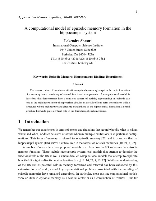
1 Appeared in Neurocomputing,38-40:889-897A computational model of episodic memory formation in thehippocampal systemLokendra ShastriInternational Computer Science Institute1947Center Street,Suite600Berkeley,CA94704,USATEL:(510)642-4274;FAX:(510)643-7684shastri@Key words:Episodic Memory;Hippocampus;Binding;RecruitmentAbstractThe memorization of events and situations(episodic memory)requires the rapid formation of a memory trace consisting of several functional components.A computational model isdescribed that demonstrates how a transient pattern of activity representing an episode canlead to the rapid recruitment of appropriate circuits as a result of long-term potentiation withinstructures whose architecture and circuitry match those of the hippocampal formation,a neuralstructure known to play a critical role in the formation of such memories.1IntroductionWe remember our experiences in terms of events and situations that record who did what to whom where and when,or describe states of affairs wherein multiple entities occur in particular config-urations.This form of memory is referred to as episodic memory[23]and it is known that the hippocampal system(HS)serves a critical role in the formation of such memories[10,21,4,22].A number of researchers have proposed models to explain how the HS subserves the episodic memory function.These include macroscopic system-level models that attempt to describe the functional role of the HS as well as more detailed computational models that attempt to explicate how the HS might realize its putative function(e.g.,[11,14,22,8,13,12].While our understanding of the HS and its potential role in memory formation and retrieval has been enhanced by this extensive body of work,several key representational problems associated with the encoding of episodic memories have remained unresolved.In particular,most existing computational models view an item in episodic memory as a feature vector or as a conjunction of features.But forreasons summarized below,such a view of episodic memory is inadequate for encoding events and situations(also see[16,18]).First,events are relational objects,and hence,cannot be encoded as a conjunction of features. Consider an event described by“John gave Mary a book in the library on Tuesday”.This event cannot be encoded by simply associating“John”,“Mary”,“a Book”,“Library”,“Tuesday”and“give”since such an encoding would be indistinguishable from that of the event“Mary gave John a book in the Library on Tuesday”.In order to make the necessary distinctions,the memory trace of an event should specify the bindings between the entities participating in the event and the roles they play in the event.For example,the encoding of should specify the following role-entity bindings:(giver=John,recipient=Mary,give-object=a-Book,temporal-location=Tuesday,location=Library).Second,the memory trace of an event should be responsive to partial cues,but at the same time,it should be capable of distinguishing between the memorized event and other highly similar events.For example,the memory trace of should respond positively to a partial cue“John gave Mary a book,”but not to a cue“John gave Susan a book in the library on Tuesday”even though the latter event shares all,but one,bindings with.Third,during retrieval,the memory trace of an event should be capable of reactivating the bind-ings associated with the event so as to recreate an active representation of the event.In particular, the memory trace of an event should support the retrieval of specific components of the event.For example,the memory trace of should be capable of differentially activating John in responseto the cue“Who gave Mary a book?”It can be shown that in order to satisfy all of the above representational requirements,the mem-ory trace of an event must incorporate functional units that serve as binding-detectors,binding-error-detectors,binding-error-integrators,relational-instance-match-indicators,and binding-reinstators [18].Moreover,as explained in[18],it is possible to evoke an articulated representation of an eventby reinstating the bindings describing the event and activating the web of semantic and procedu-ral knowledge with these bindings.Cortical circuits encoding sensorimotor schemas and generic “knowledge”about actions such as give and entities such as persons,books,libraries,and Tuesday can recreate the necessary gestalt and details about the event“John gave Mary a book on Tuesdayin the library”upon being activated with the small number of bindings associated with this event.This article partially describes a computational model,SMRITI,that demonstrates how a tran-sient pattern of activity representing an event can lead to the rapid formation of appropriate func-tional units as a result of long-term potentiation(LTP)[2]within structures whose architecture and circuitry match those of the HS.The model shows that the seemingly idiosyncratic architecture of the HS and the existence of different types of inhibitory interneurons,and different types of local inhibitory circuits in the HS,are ideally suited for the recruitment of the necessary functional units.A detailed description of the model appears in[18].Subcortical areas including amygdala, septal nucleithalamus, hypothalamus . . .Higher order sensory and polysensory association areas DG CA3CA2CA1SC EC Figure 1:Summary of major pathways interconnecting the components of the hippocampal system.Note the multiple pathways from EC to CA1,CA2,CA3,and SC.Also note the backprojections from CA1and SC to EC.The HS also receives a wide array of subcortical inputs (not shown).The subicular complex (SC)has been depicted as a single monolithic component for simplicity.See text for detail.Abbreviations:HS,hippocampal system;DG,dentate gyrus;EC,entorhinal cortex;SC,subicular complex.1.1The hippocampal systemThe hippocampal system (HS)refers to a heterogeneous collection of neural structures including the entorhinal cortex (EC),the dentate gyrus (DG),Ammon’s horn (or the hippocampus proper),and the subicular complex (SC).Ammon’s horn consists of fields CA1,CA2,and CA3,and the SC consists of the subiculum,presubiculum,and parasubiculum regions.Note that CA2is often merged with CA3in the animal literature,but is a distinct field of Ammon’s horn,especially in humans and other primates [5].Fig.1depicts a schematic of the major pathways interconnecting the components of the HS.EC serves as the principal portal between the HS and the rest of the cortex.Higher-order unimodal sensory areas as well as polymodal association areas project to upper layers of EC (e.g.,[24]).In turn,the upper layers of EC project to DG,CA3,CA2,CA1,and SC.Moreover,DG projects to CA3,CA3projects to CA2and CA1,CA2projects to CA1,and CA1projects to SC.CA1and SC project back to the deeper layers of EC which in turn project back to the high-level corticalareas that project to EC.Thus activity originating in high-level cortical regions converges on the HS via EC,courses through the complex loop formed by the pathways of the HS,and returns back to high-level cortical regions from where it had originated.In addition to the forward pathways mentioned above,there also exist pathways from CA2and CA3to DG,and recurrent connections within DG,CA3,CA2,and to a lesser extent,within CA1. Moreover,each region of the HS contains a variety of inhibitory interneurons that in conjunction with principal cells give rise to well-defined feedback and feedforward inhibitory local circuits. The HS also receives a rich set of afferents from subcortical areas that mediate arousal and other autonomic,emotional,and motivational aspects of behavior.These inputs can communicate the affective significance of an experience/stimulus to the HS.1.2Long-Term PotentiationLTP refers to long-term activity dependent increase in synaptic strength and is believed to underlie memory formation[2].In particular,convergent activity at multiple synapses that share the same postsynaptic cell can lead to their associative LTP.The proposed computational model uses a highly idealized,but computationally effective,form of associative LTP.In brief,the occurrence of LTP in the model is governed by the following parameters:the potentiation threshold,the weight increment,the window of synchrony,the repetition factor,and the maximum inter-activity interval.Consider a set of synapses sharing the same postsynaptic cell. Convergent presynaptic activity at’s can lead to associative LTP of naive’s and increase their weights by if the following conditions hold:(i)the total(convergent)activity arriving at’s exceeds,(ii)this activity is synchronous,i.e.,arrives with a maximum lead/lag of,(iii)such synchronous activity repeats at least times,and(iv)the interval between two successive arrivals of convergent activity is at most.It has been shown[17]that recruitment learning algorithms [6,15]proposed for one-shot learning in connectionist networks can befirmly grounded in LTP.2A System-level description of the modelAt a macroscopic level,the functioning of the model may be described as follows.Our cognitive apparatus construes our experiences as a stream of events and situations and these are expressed as transient and distributed patterns of activity over high-level cortical circuits(HLCCs).HLCCs in turn project to EC and give rise to transient patterns of activity.The resulting activity in EC can be viewed as the presentation of an event to the HS by HLCCs for possible memorization.Alternately, HLCCs may present an event to the HS as a“query”and expect a certain type of response from the HS if the query matches a previously memorized item,and a qualitatively different type of response if it does not.At a macroscopic level of description,the cortico-hippocampal interactionenvisioned here is similar to that assumed by other models of the HS-based memory system(e.g., [11,7,4]).The transient activity injected into EC propagates around the complex loop consisting of EC, DG,CA3,CA2,and CA1,SC,and back to EC,and triggers a sequence of synaptic changes in these structures.The model demonstrates that such synaptic changes can transform the transient pattern of activity into a persistent structural encoding(i.e.,a memory trace)composed of the requisite functional circuits mentioned in Section1.The level of significance of a presented event determines the mass,i.e.,the number of cells,recruited for encoding an event.The activity in EC resulting from the activity arriving from CA1and SC constitutes the response of the HS. The reentrant activity in EC in turn propagates back to HLCCs and completes a cycle of cortico-hippocampal interaction.Note that all entities and generic relations and their roles are expressed in various HLCCs. Only the functional units listed in Section1that are required for the encoding of specific events involving these entities,generic relations,and roles are encoded within the HS.2.1Functional architecture of SMRITIThe mapping between the functional units comprising each memory trace and the component re-gions of the HS is as follows:(refer to Fig.1).Linking cells in EC.These cells connect the HLCC based representations of entities,generic relational structures and their roles to the HS.Binding-detector cells in DG,Binding-error-detector circuits in CA3,Binding-error-integrator cells in CA2,Relational-match-indicator circuits in CA1for detecting a match between a cue and the memorized event based on the activity of the above cells and circuits,andBinding-reinstator cells in SC.Several“copies”of each functional cell and circuit are recruited during the memorization of an event leading to a highly redundant encoding of the event.The recruitment of binding-detector cells and binding-error-detector circuits is described in detail in[16].The recruitment of other functional units is discussed in[18].The transient encoding of an event or a situationThe model posits that the dynamic encoding of an event situation is a transient pattern of rhythmic activity.A role-entity binding is expressed within this activity by the synchronousfiring of cells associated with the bound role and entity[19,25,20]).It is speculated that the dynamic expression of role-entity bindings may involve band activity(minor cycle)and blocks of repeated activity (major cycle)may correspond to band activity(cf.[3]).3ResultsSimulations of the model containing1000-1500cells and8,000-15,000links have been performed to verify that the functional units are recruited as prescribed by the model.However,these sim-ulations do not reveal properties of the model arising from its large scale.To explicate these properties,a detailed quantitative analysis of the model has been carried out using plausible val-ues of system parameters.The system specification involves over75parameters which specify among other things,region and projectivefield sizes,the ratio of pyramidal cells to various types of inhibitory interneurons,firing thresholds,time course of epsps,refractory periods,and the con-ditions governing the induction of LTP.In particular,the calculations assume that DG,CA3,CA2, CA1,and SC contain15million,2.7million,800,000,15million,and1million principal cells, respectively,the ratio of principal cells to inhibitory cells is about10:1,and the size of EC DG and DG CA3projectivefields are17,000and14,respectively.These choices are based in part on data provided in[1][26].The results of the quantitative analysis show that extremely robust memory traces can be formed even if one assumes an episodic memory capacity of75,000distinct events consisting of300,000bindings.Some of the results of this quantitative analysis are displayed in Table1.The memory traces formed in the model exhibit a strong form of pattern separation and differentiate between two events even though they match along all but one dimension.This can be seen from the data presented in Fig.2which shows the response of relation-match-indicator(remind)cells in CA1to cues containing different numbers of binding-errors.Thefiring of remind cells in re-sponse to a cue signals a match between the cue and the encoded event.Ideally these cells should fire if and only if a cue has zero binding-errors with respect to the event encoded by the memory trace.In keeping with the desired behavior,the response of remind cells is sharply lower in all the binding-error conditions compared to that in the match condition.Since remind cells lie at the apex of the memory trace of an event,their response is affected by cross-talk and errors in all preceding functional units.Consequently,the robust response of remind cells is significant.re-trieval cue and the memorized event.Condition X refers to a retrieval cue involving a different type of event(e.g.,if is an event involving the act of“buying”,then a cue involving acts other than“buying”(say walking)would correspond to a cue involving a different type of event).Statistic CA3CA1binder bei reinstate195.0288.49845.87195.0213.48137.29Table1:Pfail denotes the probability that suitable cells or circuits will not be found in a target region for recruitment as a functional unit during the memorization of the event“John gave Mary a book in the library on Tuesday.”E candidate denotes the expected number of cells or circuits that receive adequate connections,and hence,are candidates for recruitment as a functional unit.E recruits specifies the expected number of candidate cells or circuits that will be recruited for each functional unit.This number indicates the expected number of“copies”of each functional unit in the memory trace of E1formed in the HS.The ratio of the number of candidate cells to the number of recruited cells is governed by inhibition from Type-1interneurons.Abbreviations:DG: dentate gyrus;SC:Subicular complex;binder:binding-detector cells;bed:binding-error-detector circuits;bei:binding-error-integrator cells;remind:relation-match-indicator circuits;reinstate: binding-reinstator cells.4PredictionsThe model predicts that significant damage to EC will lead to a catastrophic failure in the formation and retrieval of episodic memories.Damage to DG granule cells will lead to erroneous“don’t know”responses(forgetting).Large scale loss of CA3pyramids or loss of perforant path inputs to CA3will lead to false positive responses(spurious memories).Large scale loss of mossyfiber inputs or loss of CA3interneurons will lead to erroneous“don’t know”responses(forgetting).Loss of CA1pyramidal cells will lead to catastrophic forgetting,but loss of CA1inhibitory interneurons will lead to false positive responses.Subjects with damage to SC will have good recognition memory,but impaired recall,and will have difficulty responding to wh-questions.Finally,subjects with damage to CA1,but with intact EC,DG and CA3regions will continue to generate binding-error signals,and hence,continue to detect novelty[9]even though they may be amnesic.5ConclusionThe proposed computational model explains how a transient pattern of activity representing an event can lead to the formation of a functionally adequate memory trace in the HS.The memory traces capture the relational aspects of events and situations.They can differentiate between highly similar events and respond to partial cues.The model accounts for the idiosyncratic architecture and local circuitry of the HS and provides a rationale for its components and projections.It sug-gests specific and significantly different functional roles for regions CA3,CA2,CA1,and SC than those suggested by existing models.While most models of the HS view CA3as an associative memory,this work suggests that(i)a key representational role of CA3may be the detection of binding errors and(ii)CA3interneurons may play a critical role in the formation of binding-error detector circuits critical to the proper functioning of episodic memory and novelty detection.References[1]D.G.Amaral and M.P.Witter,Hippocampal Formation,in:G.Paxinos,ed.,The Rat NervousSystem,second,edition,(Academic Press,London,1995)443-493.[2]T.V.P.Bliss and G.L.Collingridge,A synaptic model of memory:long-term potentiation inthe hippocampus.Nature361(1993)31-39.[3]J.J.Chrobak and G.Buzsaki,Gamma Oscillations in the Entorhinal Cortex of the Freely Be-having Rat.J.Neurosci.,18(1998)388-398.[4]N.J.Cohen and H.Eichenbaum,Memory,Amnesia,and the Hippocampal System(M.I.T.Press,Cambridge,Massachusetts,1993).[5]H.M.Duvernoy,The Human Hippocampus.(J.F.Bergmann,Munich,1988).[6]J.A.Feldman,Dynamic connections in neural networks.Bio-Cybernet.46(1982)27-39.[7]E.Halgren,Human hippocampal and amygdala recording and stimulation:evidence for aneural model of recent memory,in:L.R.Squire and N.Butters,eds.,Neuropsychology of Memory(Guilford Press,New York,1984)165-182.[8]M.E.Hasselmo,B.P.Wyble and G.V.Wallenstein,Encoding and retrieval of episodic mem-ories:Role of cholinergic and GABAergic modulation in the hippocampus,Hippocampus6 (1996)693-708.[9]R.T.Knight,Contribution of human hippocampal region to novelty detection.Nature382(1996)256-259.[10]J.O’Keefe and L.Nadel,The hippocampus as a cognitive map(Clarendon Press,Oxford,1978).[11]D.Marr,Simple memory:a theory for archicortex,Phil.Trans.R.Soc.B262(1971)23-81.[12]J.M.J.Murre,TraceLink:a model of amnesia and consolidation of memory.Hippocampus6(1996)674–684.[13]R.C.O’Reilly and J.L.McClelland,Hippocampal Conjunctive Encoding Storage,and Re-call:Avoiding a Tradeoff,Technical Report S.94.4,Carnegie Mellon University,Pitts-burgh,PA,1994.[14]N.A.Schmajuk and J.J.DiCarlo,Stimulus configuration,classical conditioning,and hip-pocampal function.Psych Rev.99(1992)268-305.[15]L.Shastri,Semantic Networks:An evidential formalization and its connectionist realization,(Morgan Kaufamnn,Los Altos,CA,1988).[16]L.Shastri,Recruitment of binding and binding-error detector circuits via long-term potentia-tion,Neurocomputing26-27(1999)865-874.[17]L.Shastri,Biological grounding of recruitment learning and vicinal algorithms in long-termpotentiation and depression.Technical Report TR-99-009,International Computer Science Institute,Berkeley,CA,1999.[18]L.Shastri,From transient patterns to persistent structures:a model of episodic memory for-mation via cortico-hippocampal interaction.Submitted.[19]L.Shastri and V.Ajjanagadde.From simple associations to systematic reasoning.connection-ist representation of rules,variables,and dynamic bindings using temporal synchrony.Behav.Brain Sci.16(1993)417-494.[20]W.Singer and C.M.Gray,Visual feature integration and the temporal correlation hypothesis.Ann.Rev.Neurosci.18(1995)555-586.[21]L.R.Squire,Memory and the hippocampus:A synthesis fromfindings with rats,monkeys,and humans.Psych.Rev.99(1992)195-231.[22]A.Treves and E.T.Rolls,Computational analysis of the role of the hippocampus in memory.Hippocampus4(1994)374-391.[23]E.Tulving,Elements of Episodic Memory(Clarendon Press,Oxford,1978).[24]G.W.Van Hoesen,The primate hippocampus gyrus:New insights regarding its cortical con-nections.Trends Neurosci.5(1982)345-350.[25]C.von der Malsburg.Am I thinking assemblies?in:G.Palm and A.Aertsen,eds.,BrainTheory(Springer-Verlag,Berlin,1986).[26]M.J.West,Stereological studies of the hippocampus:a comparison of the hippocampal sub-divisions of diverse species including hedgehogs,laboratory rodents,wild mice and men,in:Episodic Memory Formation in the Hippocampal System11 J.Storm-Mathisen,J.Zimmer,and O.P.Ottersen,eds.,Progress in Brain Research:Under-standing the brain through the hippocampus(Elsevier Science,Amsterdam,1990)13-36.Acknowledgments:This work was supported by NSF grants9720398and9970890.。

工程英语测试题及答案一、选择题（每题2分，共20分）1. What is the term used to describe the process of turning raw materials into finished products?A. FabricationB. AssemblyC. MachiningD. Casting答案：A2. The primary function of a ________ is to convert electrical energy into mechanical energy.A. MotorB. GeneratorC. TransformerD. Inverter答案：A3. In engineering, the term "stress" refers to:A. The internal resistance of a material to deformationB. The force applied to a materialC. The change in shape of a materialD. The rate of change of force答案：A4. Which of the following is not a type of welding process?A. Arc weldingB. Gas weldingC. Ultrasonic weldingD. Friction welding答案：C5. The process of designing and building a structure is known as:A. EngineeringB. ArchitectureC. ConstructionD. All of the above答案：D6. What does the abbreviation "CAD" stand for in the field of engineering?A. Computer-Aided DesignB. Computer-Aided DraftingC. Computer-Aided DevelopmentD. Computer-Aided Documentation答案：A7. The SI unit for pressure is:A. PascalB. NewtonC. JouleD. Watt答案：A8. A ________ is a type of joint that allows for relative movement between connected parts.A. Rigid jointB. Revolute jointC. Fixed jointD. Pin joint答案：B9. The process of removing material from an object to achieve the desired shape is known as:A. MachiningB. CastingC. ForgingD. Extrusion答案：A10. In engineering, the term "specification" refers to:A. A detailed description of the requirements of aprojectB. A list of materials to be used in a projectC. The estimated cost of a projectD. The timeline for a project答案：A二、填空题（每题1分，共10分）11. The ________ is the process of cutting a flat surface ona material.答案：sawing12. A ________ is a type of bearing that allows for rotation.答案：ball bearing13. The term "gearing" refers to the use of gears to transmit ________.答案：motion14. The ________ is the study of the properties of materials.答案：material science15. In a hydraulic system, a ________ is used to control the flow of fluid.答案：valve16. The ________ is the process of heating and cooling a material to alter its physical properties.答案：heat treatment17. The ________ is a tool used to measure the hardness of a material.答案：hardness tester18. A ________ is a type of joint that connects two parts ata fixed angle.答案: hinge joint19. The ________ is the process of joining two pieces ofmetal by heating them to a molten state.答案：fusion welding20. The ________ is the study of the behavior of structures under load.答案：structural analysis三、简答题（每题5分，共30分）21. Define the term "mechanical advantage" in engineering.答案：Mechanical advantage is the ratio of output force to input force in a simple machine, indicating how much the machine amplifies the force applied to it.22. Explain the concept of "factor of safety" in engineering design.答案：The factor of safety is a ratio used in engineering to ensure that a structure or component can withstand loads beyond the maximum expected in service, providing a margin of safety against failure.23. What is the purpose of a "stress-strain curve" in material testing?答案：A stress-strain curve is a graphical representation of the relationship between the stress applied to a material and the resulting strain, used to determine the material's mechanical properties such as elasticity, yield strength, and ultimate strength.24. Describe the difference between "static" and "dynamic" loads in engineering.答案：Static loads are constant forces that do not changeover time, while dynamic loads are forces that vary in magnitude or direction over time, often due to movement or vibrations.25. What is "creep" in the context of material behavior under load?答案：Creep。

Rural Revitalization32DEVELOPMENT OF SMALL CITIES & TOWNSVOL.39 NO.6 JUN. 2021小城镇建设2021年 第39卷 第6期————————————————————————————————————————————————————————基金项目： 国家自然科学基金项目“ 中老经济走廊双边沿线城镇地区合作发展的空间应对策略研究”（编号：D1218006）； 教育部国别与区域研究基金项目“城市规划智能决策关键支持技术”（编号：19GBQY083）。

作者简介：高俊阳，华中科技大学建筑与城市规划学院博士研究生。

储梁，江苏省城市规划设计研究院设计师。

传统农区山地乡村聚落空间形态认知的核心与层次——基于生产生活视角高俊阳 储 梁 刘合林摘要：乡村聚落空间形态是聚落居民长期生产生活下人地关系的外在表征，以小农经济为主的农业生产收入依然是传统农区山地乡村居民的重要生计来源。

对于耕地的强“依附”决定了传统农区山地乡村聚落基本单元形态。

以往的乡村居民点迁并规划往往忽视了传统农区山地乡村聚落的这种强“依附”作用。

国土空间背景下的山地乡村村庄规划中居民点面临着大量的撤村并点需求。

而基于村民生计出发的聚落空间形态的认知是传统农区山地乡村规划的前提和基础。

笔者从聚落自组织的内在动力——生产生活视角切入，认为传统农区山地聚落空间形态认知的核心是“人地关系”。

在此基础上构建了空间形态认知的一般逻辑和层次：“宏观格局—人地平衡单元”“中观村落—农业生产单元”“微观宅院—日常生活单元”，并以若干典型案例阐释说明，以期为国土空间背景下传统农区山地聚落所面临的居民点整合提供自下而上的认知参考和启示。

关键词：山地乡村聚落；空间形态；生产生活；人地关系doi：10.3969/j.issn.1009-1483.2021.06.005 中图分类号：TU982.29文章编号：1009-1483（2021）06-0032-08 文献标识码：A The Core and Level of Spatial Form Cognition of Mountain Rural Settlements in Traditional Agricultural Areas: Based on the Perspective of Production and Life GAO Junyang, CHU Liang, LIU Helin[Abstract] The spatial form of rural settlements is the external representation of the relationship between human and land in the long-term production and life of the residents in the settlements. The agricultural production income, which is mainly based on small-scale peasant economy, is still an important source of livelihood for the residents in the traditional agricultural mountainous areas. The strong 'attachment' to arable land determines the basic unit form of mountain rural settlements in traditional agricultural areas. In the past, the relocation and planning of rural settlements often ignored the strong 'attachment' function of rural settlements in traditional rural areas. In the context of territorial spatial planning, the rural settlements in mountainous areas are faced with a large number of demands for village removal and location. The cognition of the spatial form of settlements based on the villagers' livelihood is the premise and foundation of the traditional mountainous and rural planning in agricultural areas. From the perspective of production and life, along with the inner motive force of self-organization of settlements, the author believes that the core of spatial form cognition of mountain settlements in traditional agricultural areas is 'man-land relationship'. On this basis, the general logic and levels of spatial form cognition are constructed, such as 'macro pattern-human-land balance unit', 'medium village-agricultural production unit', 'micro house-daily life unit', and illustrated with several typical cases, in order to provide a bottom-up cognitive reference and inspiration for the integration of settlements faced by traditional mountainous rural areas under the background of territorial space.[Keywords] mountain rural settlement; space form; production and life; man- land relationship乡村振兴33DEVELOPMENT OF SMALL CITIES & TOWNSVOL.39 NO.6 JUN. 2021小城镇建设2021年 第39卷 第6期引言乡村聚落又称乡村居民点，是指乡村地区各种形式的人口居住场所，即村落。

有百分比的英文作文范文Title: The Significance of Percentages in Everyday Life In the intricate tapestry of our daily existence, percentages play a pivotal role. They are the silent architects of our decisions, shaping our understanding of the world and influencing our actions. From the mundane tasks of managing household budgets to the complex calculations of scientific research, percentages are an essential tool for comprehension and analysis.At its core, a percentage represents a fraction of a whole, expressed as a number between 0 and 100. This simple concept has profound implications in various aspects of life. For instance, in the realm of finance, percentages are used to calculate profits, losses, interest rates, and taxes. A savvy investor would carefully analyze the percentage returns of different investment options to make informed decisions. Similarly, households rely on percentages to budget their expenses, ensuring that essential expenses are covered while leaving room for discretionary spending.In the field of education, percentages are used to assess student performance and compare it with national or international standards. A student's grade point average (GPA) is calculated using percentages, providing a quantitative measure of academic achievement. This information is crucial for colleges and universities to assess applicants and make admission decisions. Additionally, percentages are used to track progress in learning and identify areas where students may need additional support.The importance of percentages extends beyond the financial and educational domains. In the world of sports, percentages are used to analyze team performance, player statistics, and probabilities of winning. In politics, percentages are employed to gauge voter turnout, election results, and public opinion. In healthcare, they help doctors and researchers understand the prevalence of diseases, the effectiveness of treatments, and the overall health status of a population.Moreover, percentages play a significant role in data analysis and statistics. They allow researchers to identifypatterns, trends, and outliers in large datasets. By comparing percentages across different groups or over time, researchers can gain insights into complex social, economic, and environmental issues.However, it's crucial to remember that percentagesalone can be misleading. They are just one tool in the toolbox of analysis, and should be used in conjunction with other qualitative and quantitative information. A high percentage does not automatically mean something is good or bad; it merely provides a numerical representation of a relationship.In conclusion, percentages are a powerful tool that permeates every aspect of our lives. They help us understand, analyze, and make decisions in a wide range of contexts. Whether we are managing our finances, assessing our academic performance, analyzing sports statistics, or understanding complex social issues, percentages provide a valuable lens for comprehension. As we navigate the complexities of the modern world, it's essential to embrace and harness the power of percentages to enrich our understanding and enhance our decision-making abilities.。

erdERD (Entity-Relationship Diagram) is a visual representation of the relationships between different entities in a system. It is often used in database design to map out the structure of a relational database. ERD helps to identify the entities, attributes, and relationships between various entities in a system. This document aims to provide an in-depth understanding of ERD and its components.1. Introduction1.1 What is ERD?ERD, short for Entity-Relationship Diagram, is a modeling technique used to represent the logical structure and relationships between different entities in a system. It is commonly used in database design to create a blueprint for a relational database.1.2 Importance of ERDERD is crucial in database design as it helps in understanding the logical structure of the system. It provides a visual representation of the entities and their relationships, which aids in database development and maintenance. ERD helps in identifying the key entities, attributes, and relationships,which are essential for ensuring data integrity and efficient data retrieval.2. Components of ERD2.1 EntitiesEntities are the fundamental building blocks of an ERD. They represent real-world objects or concepts that have attributes and exist independently. Each entity in an ERD is represented by a rectangle, and their names are mentioned within the rectangle.2.2 AttributesAttributes define the properties or characteristics of an entity. They provide additional information about an entity. Each attribute is depicted as an oval shape connected to its respective entity. Attributes can be classified as simple attributes, composite attributes, or multi-valued attributes.2.3 RelationshipsRelationships represent the associations or connections between entities. They depict the way entities relate or interact with each other. Relationships are depicted by diamond-shaped symbols. The cardinality and degree ofrelationships can be represented using notations within the diamond shape.3. Types of Relationships3.1 One-to-One RelationshipIn a one-to-one relationship, each record in one entity is associated with only one record in another entity. For example, a person can have only one passport, and a passport can be issued to only one person.3.2 One-to-Many RelationshipIn a one-to-many relationship, a single record in one entity can be associated with multiple records in another entity. For example, a customer can have multiple orders, but each order belongs to only one customer.3.3 Many-to-One RelationshipIn a many-to-one relationship, multiple records in one entity can be associated with a single record in another entity. For example, multiple employees can work in the same department.3.4 Many-to-Many RelationshipIn a many-to-many relationship, multiple records in one entity can be associated with multiple records in another entity. For example, students can enroll in multiple courses, and each course can have multiple students.4. Cardinality and Multiplicity4.1 CardinalityCardinality determines the number of occurrences of one entity that can be associated with the number of occurrences of another entity in a relationship.4.2 MultiplicityMultiplicity specifies the minimum and maximum number of associations between entities in a relationship. It defines the range of occurrences allowed between entities.5. Developing an ERD5.1 Identify EntitiesThe first step in developing an ERD is to identify and define the entities involved in the system. Entities should represent the key objects or concepts that are relevant to the system being modeled.5.2 Define AttributesOnce the entities are identified, the next step is to define the attributes for each entity. Attributes provide additional information about the entities and help in distinguishing between different instances of an entity.5.3 Determine RelationshipsAfter defining the attributes, the relationships between entities need to be determined. Understanding the associations and interactions between entities is crucial for accurately representing the system.5.4 Refine the ERDFinally, the ERD should be refined and validated to ensure its accuracy and completeness. The relationships, cardinality, and multiplicity should be reviewed to verify that they accurately represent the business rules and requirements of the system.6. ConclusionERD is a powerful tool used in database design to model the relationships between entities in a system. It provides a clear and concise representation of the logical structure and relationships, aiding in the development and maintenance of databases. By understanding the key components of an ERD,such as entities, attributes, and relationships, one can effectively design and manage relational databases.。

材料物理英语Material Physics English。

Material physics is a branch of physics that focuses on the study of the physical properties of materials, such as electrical, magnetic, and optical properties, as well as the relationship between the structure and properties of materials. In this document, we will explore some key concepts and terms in material physics, and provide English translations for these terms to help you better understand and communicate about this subject in English.1. Crystal Structure。

Crystal structure refers to the arrangement of atoms or molecules in a crystalline material. The crystal structure of a material determines many of its properties, such as its mechanical, thermal, and electrical behavior. In material physics, crystal structures are often described using terms such as unit cell, lattice, and symmetry operations.2. Band Gap。

AN INTRODUCTION TO GENERALIZED LINEAR MIXED MODELSStephen D.KachmanDepartment of Biometry,University of Nebraska–LincolnAbstractLinear mixed models provide a powerful means of predicting breeding values.However,for many traits of economic importance the assumptions of linear responses,constant variance,and normality are questionable.Generalized linear mixed modelsprovide a means of modeling these deviations from the usual linear mixed model.Thispaper will examine what constitutes a generalized linear mixed model,issues involvedin constructing a generalized linear mixed model,and the modifications necessary toconvert a linear mixed model program into a generalized linear mixed model program.1IntroductionGeneralized linear mixed models(GLMM)[1,2,3,6]have attracted considerable at-tention over the years.With the advent of SAS’s GLIMMIX macro[5],generalized linear mixed models have become available to a larger audience.However,in a typical breeding evaluation generic packages are too inefficient and implementations in FORTRAN or C are needed.In addition,GLMM’s pose additional challenges with some solutions heading for ±∞.The objective of this paper is to provide an introduction to generalized linear mixed models.In section2,I will discuss some of the deficiencies of a linear model.In sec-tion3,I will present the generalized linear mixed model.In section4,I will present the estimation equations for thefixed and random effects.In section5,I will present a set of estimating equations for the variance components.In section6,I will discuss some of the computational issues involved when these approaches are used in practice.2Mixed modelsIn this section I will discuss the linear mixed model and when the implied assumptions are not appropriate.A linear mixed model isy|u∼N(Xβ+Zu,R)where u∼N(0,G),X and Z are known design matrices,and the covariance matrices R and G may depend on a set of unknown variance components.The linear mixed model assumes that the relationship between the mean of the dependent variable y and thefixed and random effects can be modeled as a linear function,the variance is not afunction of the mean,and that the random effects follow a normal distribution.Any or all these assumptions may be violated for certain traits.A case where the assumption of linear relationships is questionable is pregnancy rate. Pregnancy is a zero/one trait,that is,at a given point an animal is either pregnant(1)or is not pregnant(0).For example,a change in management that is expected to increase pregnancy rate by.1in a herd with a current pregnancy rate of.5would be expected to have a smaller effect in a herd with a current pregnancy rate of.8;that is,a treatment,an environmental factor,or a sire would be expected to have a larger effect when the mean pregnancy rate is.5than when the pregnancy rate is.8.Another case where the assumption of a linear relationship is questionable is the anal-ysis of growth.Cattle,pigs,sheep,and mice have similar growth curves over time;that is,after a period of rapid growth they reach maturity and the growth rate is considerably slower.The relationship of time with weight is not linear,with time having a much larger effect when the animal is young and a very small effect when the animal is mature.The assumption of constant variance is also questionable for pregnancy rate.When the predicted pregnancy rate,µ,for a cow is.5the variance isµ(1−µ)=.25.If on the other hand the predicted pregnancy rate for a cow is.8the variance drops to.16.For some production traits the variance increases as mean level of production increases.The assumption of normality is also questionable for pregnancy rate.It is difficult to justify the assumption that the density function of a random variable which only takes on two values is similar to a continuous bell shaped curve with values ranging from−∞to +∞.A number of approaches have been taken to address the deficiencies of a linear mixed model.T ransformations have been used to stabilize the variance,to obtain a linear rela-tionship,and to normalize the distribution.However the transformation needed to stabilize the variance may not be the same transformation needed to obtain a linear relationship. For example a log transformation to stabilize the variance has the side effect that the model on the original scale is multiplicative.Linear and multiplicative adjustments are used to adjust to a common base and to account for heterogeneous variances.Multiple trait analysis can be used to account for heterogeneity of responses in different environ-ments.Separate variances can be estimated for different environmental groups where the environmental groups are based on the observed production.Afinal option is to ignore the deficiencies of the linear mixed model and proceed as if a linear model does hold.The above options have the appeal that they are relatively simple and cheap to im-plement.Given the robustness of the estimation procedures,they can be expected to produce reasonable results.However,these options sidestep the issue that the linear mixed model is incorrect.Specifically we have a set of estimation procedures which are based on a linear mixed model and manipulate the data to make itfit a linear mixed model. It seems more reasonable to start with an appropriate model for the data and use an es-timation procedure derived from that model.A generalized linear mixed model is a model which gives us extraflexibility in developing an appropriate model for the data[1].σFixedEffects h(η)InverseLink LinearPredictor GComponentsVarianceRandomEffectsβRMean Observations Figure 1:Symbolic representation of a generalized linear mixed model.3A Generalized Linear Mixed ModelIn this section I will present a formulation of a generalized linear mixed model.It differs from presentations such as [1]in that it focuses more on the inverse link function rather than the link function to model the relationship between the linear predictor and the conditional mean.Generalized linear mixed models also includes the nonlinear mixed models of [4].Figure 1provides a symbolic representation of a generalized linear mixed model.As in a linear mixed model,a generalized linear mixed model includes fixed effects,β,with (e.g.,management effect);random effects,u ∼N(0,G ),(e.g.,breeding values);design matrices X and Z ;and a vector of observations,y ,(e.g.,pregnancy status)for which the conditional distribution given the random effects has mean,µ(e.g.,mean pregnancy rate),and covariance matrix,R ,(e.g.,variance of pregnancy status is µ(1−µ)).In addition,a generalized linear mixed model includes a linear predictor,η,and a link and/or inverse link function.In addition,the conditional mean,µ,depends on the linear predictor through an inverse link function,h (·),and the covariance matrix,R ,depends on µthrough a variance function.For example,the mean pregnancy rate,µ,depends on the effect of management and the breeding value of the animal.The management effect and breeding value actadditively on a conceptual underlying scale.Their combined effect on the underlying scale is expressed as the linear predictor,η.The linear predictor is then transformed to the observed scale(i.e.,mean pregnancy rate)through an inverse link function,h(η).A typical transformation would beh(η)=eη1+eη.3.1Linear Predictor,ηAs with a linear mixed model,thefixed and random effects are combined to form a linear predictorη=Xβ+Zu.With a linear mixed model the model for the vector of observations y is obtained by adding a vector of residuals,e∼N(0,R),as followsy=η+e=Xβ+Zu+e.Equivalently,the residual variability can be modeled asy|u∼N(η,R).Unless y has a normal distribution,the formulation using e is clumsy.Therefore,a gen-eralized linear mixed model uses a second approach to model the residual variability.The relationship between the linear predictor and the vector of observations in a generalized linear mixed model is modeled asy|u∼(h(η),R)where the notation,y|u∼(h(η)R),specifies that the conditional distribution of y given u has mean,h(η),and variance,R.The conditional distribution of y given u will be referred to as the error distribution.Choice of whichfixed and random effects to include in the model will follow the same considerations as for a linear mixed model.It is important to note that the effect of the linear predictor is expressed through an inverse link function.Except for the identity link function,h(η)=η,the effect of a one unit change inηi will not correspond to a one unit change in the conditional mean;that is, predicted progeny difference will depend on the progeny’s environment through h(η).The relationship between the linear predictor and the mean response on the observed scale will be considered in more detail in the next section.3.2(Inverse)Link FunctionThe inverse link function is used to map the value of the linear predictor for observation i,ηi,to the conditional mean for observation i,µi.For many traits the inverse link function is one to one,that is bothµi andηi are scalars.For threshold models,µi is a t×1vector,T able1:Common link functions and variance functions for various distributionsDistribution Link Inverse Link v(µ)Normal Identityη1Binomial/n Logit eη/(1+eη)µ(1−µ)/nProbitΦ(η)Poisson Log eηµGamma Inverse1/ηµ2Log eηwhere t is the number of ordinal levels.For growth curve models,µi is an n i×1vector andηi is a p×1vector,where the animal is measured n i times and there are p growth curve parameters.For the linear mixed model,the inverse link function is the identity function h(ηi)=ηi. For zero/one traits a logit link functionηi=ln(µi/[1−µi])is often used,the corresponding.The logit link function,unlike the identity link function, inverse link function isµi=eηiηiwill always yield estimated means in the range of zero to one.However,the effect of a one unit change in the linear predictor is not constant.When the linear predictor is0 the corresponding mean is.5.Increasing the linear predictor by1to1increases the corresponding mean by.23.If the linear predictor is3,the corresponding mean is.95. Increasing the linear predictor by1to4increases the corresponding mean by only.03. For most univariate link functions,link and inverse link functions are increasing monotonic functions.In other words,an increase in the linear predictor results in an increase in the conditional mean,but not at a constant rate.Selection of inverse link functions is typically based on the error distribution.Table1 lists a number of common distributions along with their link functions.Other considera-tions include simplicity and the ability to interpret the results of the analysis.3.3Variance FunctionThe variance function is used to model non-systematic variability.Typically with a generalized linear model,residual variability arises from two sources.First,variability arises from the sampling distribution.For example,a Poisson random variable with mean µhas a variance ofµ.Second,additional variability,or over-dispersion,is often observed.Modeling variability due to the sampling distribution is straight forward.In Table1the variance functions for some common sampling distributions are given.Variability due to over-dispersion can be modeled in a number of ways.One approach is to scale the residual variability as var(y i|u)=φv(µi),whereφis an over-dispersion parameter.A second approach is to add a additional random effect,e i∼N(0,φ),to the linear predictor for each observation.A third approach is to select another distribution. For example,instead of using a one parameter(µ)Poisson distribution for count data,a two parameter(µ,φ)negative binomial distribution could be used.The three approaches all involve the estimation of an additional parameter,φ.Scaling the residual variability is the simplest approach,but can yield poor results.The addition of a random effect has theeffect of greatly increasing the computational costs.3.4The partsT o summarize,a generalized linear model is composed of three parts.First,a linear predictor,η=Xβ+Zu,is used to model the relationship between thefixed and random effects.The residual variability contained in the residual,e,of the linear mixed model equation is incorporated in the variance function of the generalized linear mixed model. Second,an inverse link function,µi=h(ηi),is used to model the relationship between the linear predictor and the conditional mean of the observed trait.In general,the link function is selected to be both simple and reasonable.Third,a variance function,v(µi,φ), is used to model the residual variability.Selection of the variance function is typically dictated by the error distribution that was chosen.In addition,observed residual variability is often greater than expected due to sampling and needs to be accounted for with an overdispersion parameter.4Estimation and PredictionThe estimating equations for a generalized linear mixed model can be derived in a number of ways.From a Bayesian perspective the solutions to the estimating equations are posterior mode predictors.The estimating equations can be obtained by using a Laplacian approximation of the likelihood.The estimating equations for thefixed and random effects areX H R−1HX X H R−1HZ Z H R−1HX Z H R−1HZ+G−1 βu= X H R−1y∗Z H R−1y∗(1)whereH=∂µ∂ηR=var(y|u)y∗=y−µ+Hη.Thefirst thing to note is the similarity to the usual mixed model equations.This is easier to see if we rewrite the equations in the following formX W X X W Z Z W X Z W Z+G−1 βu= X hryZ hry(2)whereW=H R−1Hhry=H R−1y∗.Unlike the mixed model equations,the estimating equations(1)for a generalized linear mixed must be solved iteratively.0.20.40.60.81-4-2024M e a n (µ)Linear Predictor (η)Figure 2:Inverse logit link function µ=e η/(1+e η).4.1Univariate LogitT o see how all the pieces fit together,we will examine a univariate binomial with a logit link function which would be an appropriate model for examining proportion data.Let y i be the proportion out of n for observation i ,a reasonable error distribution for ny i would be Binomial with parameters,n and µi .For a univariate model,the H ,R ,and W matricesare all diagonal with diagonal elements equal to ∂µi i ,ν(µi ),and W ii respectively.The variance function for a scaled Binomial random variable is ν(µi )=µi (1−µi )/n .The inverse link function is selected to model the nonlinear response of the means,µi ,tochanges in the linear predictor,ηi .The inverse link function selected is µi =e ηi 1+e ηi .The nonlinear relationship between the linear predictor and the mean can be seen in Figure 2.Changes in the linear predictor when the mean is close to .5have a larger impact than similar changes when the mean is close to 0or 1.For example,a change in the linear predictor from 0to .5changes the mean from 50%to 62%.However,a change from 2to2.5changes the mean from 88%to 92%.The weight,W ii,and scaled dependent variable,hry i,for observation i are∂µi ∂ηi =∂eηiηi∂ηi=µi(1−µi)W ii=∂µi∂ηi[ν(µi)]−1∂µi∂ηi=µi(1−µi) nµi(1−µi) µi(1−µi)=nµi(1−µi)hry i=∂µi∂ηi[ν(µi)]−1 y i−µi+∂µi∂ηiηi=n y i−µi+µi(1−µi)ηi .This can be translated into a FORTRAN subroutine as followsSUBROUTINE LINK(Y,WT,ETA,MU,W,HRY)REAL*8Y,WT,ETA,MU,W,R,VAR,Hmu=exp(eta)/(1.+exp(eta))!h(ηi)=eηi/(1+eηi)h=mu*(1.-mu)!∂µi/∂ηi=µi(1−µi)var=mu*(1.-mu)/wt!ν(µi)=µi(1−µi)/nW=(H/VAR)*H!W=Diag(H R−1H)HRY=(H/VAR)*(Y-MU)+W*ETA!hry=H R−1[y−µ+Hη]RETURNENDIn the subroutine Y=y i,WT=n,and ETA= ηi are passed to the subroutine.The sub-routine returns W=W ii,MU=µi,and HRY=hry i.In the subroutine the linesmu=exp(eta)/(1.+exp(eta))h=mu*(1.-mu)would need to be changed if a different link function was selected.The linevar=h/wtwould need to be changed if a different variance function was selected.The changes to the LINK subroutine to take into account boundary conditions will be discussed in sec-tion6.For each round of solving the estimating equations(2),a new set of linear predictors needs to be calculated.This can be accomplished during the construction of the LHS and RHS assuming solutions are not destroyed.The FORTRAN code for thisDO I=1,N!Loop to read in the N records.Read in recordETA=0!Calculate the risk factorηi=ETA based on the DO J=1,NEFF!solution for the NEFFfixed and random effects ETA=ETA+X*SOL!SOL and the design matrix X.END DOCALL LINK(Y,WT,ETA,MU,W,HRY)!Calculate µi=MU,W ii=W,and hry i=HRY!based on y i=Y,n=Wt,and ηi=ETA.Build LHS and RHSEND DO4.2Numerical exampleThe data in T able2have been constructed to illustrate the calculations involved for binomial random variables with a logit link function.A linear predictor of pregnancy rate for a cow in herd h on diet d isµhd=µ+Herd h+Diet dwhere Herd h is the effect of herd h and Diet d is the effect of diet d.For thefirst round we will use an initial estimate forηi of0.The contributions of each observation for round one is given in T able3.The estimating equations and solutions for round1are37.512.52515202.512.512.5057.50250251012.52.5155101500207.512.502002.502.5002.5µ Herd1Herd2Diet ADiet BDiet C=4053512253µ Herd1Herd2Diet ADiet BDiet C=1.2−1.04416−0.05194810.441558and η=X β=0.1038960.5974031.148051.641561.2.The new estimates of the linear predictor are used to obtain the contributions of each observation for round two given in T able4.Table2:Example data.Number PregnancyHerd Diet of Cows Rate1A20.501B30.662A40.802B50.902C10.80T able3:Contributions to the estimating equations for round one.Herd Diet y iηiµi n i W ii hry i1A0.500.520501B0.¯600.5307.552A0.800.54010122B0.900.55012.5202C0.800.510 2.53T able4:Contributions to the estimating equations for round two. Herd Diet y iηiµi n i W ii hry i1A0.50.1038960.52595120 4.98653-0.000932566 1B0.¯60.5974030.64506230 6.86871 4.751532A0.8 1.148050.759155407.3135510.03012B0.9 1.641560.83774750 6.7963514.26932C0.8 1.20.76852510 1.77894 2.449495Variance Component EstimationThe code given above assumes that the variance components are known.In this section I will discuss how estimates of the variance components can be obtained.Con-ceptually the variance component problem can be broken into two parts.Thefirst part is the estimation of the variance components associated with the random effects.The second part is the estimation of the variance components associated with the error dis-tribution.Before examining the modifications for a GLMM we will briefly review the major features of a variance component estimation program for a mixed model.5.1Mixed modelDerivative based programs for estimation of variance components under a mixed model involve the computation of quadratic forms of the predicted random effects, u Q i u, along with functions of the elements of a generalized inverse of the left hand sides,f ij(C), where C is a generalized inverse of the left hand sides in(2).For example,the univariate Fisher scoring quadratic form of the REML estimator of variance component i isu i I q i u iσiwhere u i is the q i×1vector of predicted random effects for i th set of random effects.The function of the left hand sides aref ii(C)=1σ4iq i−2tr(C ii)σ2i+tr(C ii C ii)σ4if ij(C)=1σiσjtr(C ij C ji)σiσjwhereC=C00C01 0C10C11 (1)...C r0C r1...C rris the partitioned generalized inverse of the left hand sides of(2).For the residual variance component,the quadratic form is(y−X β−Z u) I N(y−X β−Z u)σwhere N is the number of observations.The functions of the left hand sides aref i0(C)=1σ2iσ2tr(C ii)σ2i−rj=1tr(C ij C ji)σ2iσ2jf00(C)=1σ4N−p∗−q+ri=1rj=1tr(C ij C ji)σ2iσ2j.(3)5.2Modifications for GLMMThe variance components can be estimated using the approximate REML quasi-likelihood [1]which after some algebra isql (β,σ)=−12ln |V |−12ln |X H V −1HX |−12(y ∗−HXβ) V −1(y ∗−HXβ)(4)where σis the vector of variance component and V =R +HZGZ H .For the variance components associated with the random effects in G the estimating equations remain thesame except uand C are obtained using (2)instead of the usual mixed model equations.Estimation of the variance components associated with the error distribution is more problematic.The quadratic form becomes(y − µ) R −1∂R ∂φR −1(y − µ).(5)However,the corresponding functions for the left hand side in (3)for the linear mixedmodel assumes that R =I σ2o .The functions of the left hand sides for φaref 00(C )=[tr(Φ)−2tr(ΩΦ)+tr(ΩΦΩΦ)]f i 0(C )= tr(C i X H ΦHX X H ΦHZ Z H ΦHX Z H ΦHZC i ) where C i =(C i 0C i 1...C ir ),Φ=R −1∂R ∂φR −1andΩ= HX HZ CX H Z H .6Some Computational Issues While the mathematics are “straight forward,”implementation in practice is often chal-lenging.Many of the difficulties associated with generalized linear mixed models are related to either estimates going to infinity or divide by zero problems.Consider the uni-variate logit model.The calculations involve 1i i .Provided 0<µ<1this quantity is well defined.If µapproaches either zero or one,then the quantity 1µi (1−µi )approaches infinity.Estimates of µof zero or one occur when a contemporary group consists entirely of zeros or ones.Several options exist for handling this situation.One approach is to remove from the data any troublesome contemporary groups.While mathematically sound,an additional edit is needed to remove legitimate data values.A second approach is to treat contem-porary group effects as random effects.However,the decision to treat a set of effects asfixed or random should be decided from a modeling standpoint and not as an artifact of the estimation procedure.A third approach is to adjust y i away from0and1.For exam-ple,one could use(y i+∆)/(1+2∆)instead of y i.A fourth approach is based on the examination of what happens to the quantities W ii and hry i whenηi approaches infinity.Asηi→±∞,W ii→0andhry i→n(y i−µi)In the limit W ii and hry i are both well defined.One could then recode the link function as SUBROUTINE LINK(Y,WT,ETA,MU,W,HRY)REAL*8Y,WT,ETA,MU,W,R,VAR,Hif(abs(eta)>BIG)then!Check for ηi→±∞if(eta>0)then! ηi→∞⇒ µi→1mu=1.else! ηi→−∞⇒ µi→0mu=0end ifw=0! ηi→±∞⇒W ii→0hry=wt*(y-mu)!and hry i→n(y i− µi)returnend ifmu=exp(eta)/(1.+exp(eta))h=mu*(1.-mu)var=h/wtW=(H/VAR)*HHRY=(H/VAR)*(Y-MU)+W*ETARETURNENDwhere BIG is a sufficiently large,but not too large a number.For example BIG=10might be a reasonable choice.However,using W ii=0will usually result in a zero diagonal in the estimating equations.When these equations are solved,thefixed effect which was approaching infinity will be set to zero.This substitution can result in interesting convergence problems.A solution would be to“fix”the offensivefixed effect by making the following changesSUBROUTINE LINK(Y,WT,ETA,MU,W,HRY)REAL*8Y,WT,ETA,MU,W,R,VAR,Hif(abs(eta)>BIG)then!Check for ηi→±∞if(eta>0)then!−BIG≤ ηi≤BIGeta=BIGelseeta=-BIGend ifmu=exp(eta)/(1.+exp(eta))h=mu*(1.-mu)var=h/wtW=(H/VAR)*HHRY=(H/VAR)*(Y-MU)+W*ETARETURNEND6.1Additional ParametersThreshold models with more than two classes and growth curve models require more than one linear predictor per observation.In the case of a threshold model the value of an observation is determined by the usual linear predictor and a threshold linear predictor.With growth curve models animal i has n i observations.The linear predictor for animal i is a p ×1vector,where p is the the number of growth curve parameters.Unlike the univariate case,the matrices H ,W ,and R may not be diagonal.Typical structures for these matrices are:R =Diag(R i )with R i a n i ×n i residual covariance matrixH =Diag(H i )with H i a n i ×p matrix of partial derivatives H i = ∂µi 1∂ηi 1...∂µi 1∂ηip ...∂µin i i 1...∂µin i ip W =Diag(W i )with W i =H i R −1i H i .7ConclusionsGeneralized linear mixed models provide a flexible way to model production traits which do not satisfy the assumptions of a linear mixed model.This flexibility allows the researcher to focus more on selecting an appropriate model as opposed to finding manip-ulations to make the data fit a restricted class of models.The flexibility of a generalized linear mixed model provides an extra challenge when selecting an appropriate model.As a general rule the aim should be to select as simple a model as possible which does a reasonable job of modeling the data.While generalized linear mixed model programs are not as readily available as linear mixed model programs,modifications needed for a linear mixed model program should be minor.The two changes that are needed are to add a Link subroutine and to solve iteratively the estimating equations.In constructing a link subroutine it is important to handle boundary conditions robustly.When selecting a link function it is important to remember that when you get the results from the analysis,you will need to both interpret the results and to present the results in a meaningful manner.Generalized linear mixed models provide us with a very powerfulReferences[1]N.E.Breslow and D.G.Clayton.Approximate inference in generalized linear mixedmodels.J.Amer.Statist.Assoc.,88:9–25,1993.[2]B.Engel and A.Keen.A simple approach for the analysis of generalized linear mixedmodels.Statist.Neerlandica,48(1):1–22,1994.[3]D.Gianola and J.L.Foulley.Sire evaluation for ordered categorical data with a thresh-old model.G´en´et.S´el.Evol.,15(2):210–224,1983.[4]M.J.Lindstrom and D.M.Bates.Nonlinear mixed effects models for repeated mea-sures data.Biometrics,46:673–687,1990.[5]Ramon C.Littell,George liken,Walter W.Stroup,and Russell D.Wolfinger.SASSystem for Mixed Models.SAS Institute Inc.,Cary,NC,1996.[6]I.Misztal,D.Gianola,and puting aspects of a nonlinear method ofsire evaluation for categorical data.J.Dairy Sci.,72:1557–1568,1989.。