古扎拉蒂计量经济学第四版讲义Ch7 Heteroscedasticity
- 格式:pdf
- 大小:123.82 KB
- 文档页数:15

第五章 虚拟变量回归模型Dummy Variable Regression Models1、什么是虚拟变量?名义型变量又称为指标变量、分类变量、定性变量,或者虚拟变量(哑变量)。
2、方差分析模型(ANOVA models )一种类型的回归模型就是解释变量全部是虚拟变量,这样的模型称为Analysis of Variance (ANOV A) models 。
假如我们想检验东(10个省)中(12个省)西(9个省)部三个地区教师的平均收入是否不同。
对三个地区教师工资数据取算术平均值,发现不同,这种不同显著吗?一般用D 表示哑变量,设定如下的哑变量: D2 =1 代表东部省份;否则用0表示 D3 =1代表中部省份;否则用0表示可以写出如下的模型12233i i i i y D D βββε=+++ 9.2.1这类似于一般的多元回归模型的形式。
假定该模型的误差项满足通常OLS 回归的假定,对上式两边取期望,得到 对东部地区: ()2312|1,0i i i E y D D ββ===+ 对中部地区: ()2313|0,1i i i E y D D ββ===+ 对西部地区: ()231|0,0i i i E y D D β===假定回归结果为()()()2322158.622264.6151734.473:0.00000.03490.23300.0901i i i y D D p R =++=1)虚拟变量使用注意使用虚拟变量要小心,特别要注意以下几点:1)一个定性解释变量如果分成m 类,则用m-1个哑变量表示;如果分成m 类用m 个哑变量表示,则会掉进哑变量陷阱,即引起多重共线性。
该规则同样适用于两个定性解释变量的情形。
2)对于一个定性解释变量,其没有赋予值1的区间称为基准区间(base, benchmark, control, comparison, reference, or omitted category )。
⭐️经济计量学精要(第4版)/(美)古扎拉蒂大佬点个赞支持一下呗ヽ(´▽`)ノヽ(´▽`)ノヽ(´▽`)ノ经济计量学精要(第4版)/(美)古扎拉蒂•综述1.1 什么是经济计量学1.2 为什么要学习经济计量学1.3 经济计量学方法论经济计量分析步骤:(1)建立一个理论假说(2)收集数据(3)设定数学模型线性回归模型为例线性回归模型中,等式左边的变量称为应变量,等式右边的变量称为自变量或解释变量。
线性回归分析的主要目标就是解释一个变量(应变量)与其他一个或多个变量(解释变量)之间的行为关系。
简单数学模型•(4)设立统计或经济计量模型误差项u•u代表随机误差项,简称误差项。
u包括了X以外其他所有影响Y,但并未在模型中具体体现的因素以及纯随机影响。
(5)估计经济计量模型参数线性回归模型常用最小二乘法估计模型中的参数^读做"帽",表示某的估计值(6)核查模型的适用性:模型设定检验(7)检验源自模型的假设:假设检验(8)利用模型进行预测数据类型时间序列数据:按时间跨度收集得到的截面数据:一个或多个变量在某一时间点上的数据集合合并数据:既包括时间序列数据又包括截面数据面板数据:也称纵向数据、围观面板数据,即同一个横截面单位的跨期调查数据模型因果关系统计关系无论有多强,有多紧密,也决不能建立起因果关系,如果两变量存在因果关系,则一定建立在某个统计学之外的经济理论基础之上。
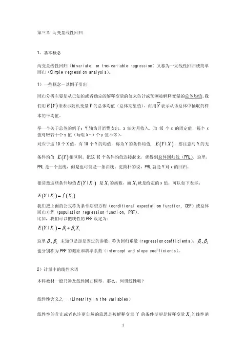
第一部分线性回归模型2.1回归的含义回归分析的主要目的:根据样本回归函数SRF估计总体回归函数PRF2.2总体回归函数(PRF):假想一例总体回归线给出了对应于自变量的每个取值相应的应变量的均值。
(总体回归线表明了Y的均值与每个X的变动关系)PRL•E(Y|xi)表示与给定x值相对应的Y的均值。
下标i代表第i个子总体。
B1、B2称为参数,也称为回归系数。
B1称为截距,B2称为斜率。
斜率系数度量了X每变动一单位,Y( 条件)均值的变化率。

第3章双变量模型:假设检验3.1 复习笔记一、古典线性回归模型古典线性回归模型假定如下:假定1:回归模型是参数线性的,但不一定是变量线性的。
回归模型形式如下:Y i=B1+B2X i+u i这个模型可以扩展到多个解释变量的情形。
假定2:解释变量X与扰动误差项u不相关。
但是,如果X是非随机的(即为固定值),则该假定自动满足。
即使X值是随机的,如果样本容量足够大,也不会对分析产生严重影响。
假定3:给定X,扰动项的期望或均值为零。
即E(u|X i)=0(3-1)假定4:u i的方差为常数,或同方差,即var(u i)=σ2(3-2)假定5:无自相关假定,即两个误差项之间不相关。
即:cov(u i,u j)=0,i≠j(3-3)无自相关假定表明误差u i是随机的。
由于假定任何两个误差项不相关,所以任何两个Y值也是不相关的,即cov(Y i,Y j)=0。
由于Y i=B1+B2X i+u i,则给定B值和X值,Y 随u的变化而变化。
因此,如果u是不相关的,则Y也是不相关的。
假定6:回归模型是正确设定的。
换句话说,实证分析的模型不存在设定偏差或设定误差。
这一假定表明,模型中包括了所有影响变量。
二、普通最小二乘估计量的方差与标准误有了上述假定就能够估计出OLS估计量的方差和标准误。
由此可知,教材式(2-16)和教材式(2-17)给出的OLS估计量是随机变量,因为其值随样本的不同而变化。
这种抽样变异性通常由估计量的方差或其标准误(方差的平方根)来度量。
教材式(2-16)和式(2-17)中OLS估计量的方差及标准误是:(3-4)(3-5)(3-6)(3-7)其中,var表示方差,se表示标准误,σ2是扰动项u i的方差。
根据同方差假定,每一个u i具有相同的方差σ2。
一旦知道了σ2,就很容易计算等式右边的项,从而求得OLS估计量的方差和标准误。
根据下式估计σ2:(3-8)其中,σ∧2是σ2的估计量,是残差平方和,是Y的真实值与估计值差的平方和,即()122212var ibiXbn xσσ==∑∑1se()b=()22222varbibxσσ==∑()2se b=22ˆ2ienσ=−∑2ie∑n -2称为自由度,可以简单地看作是独立观察值的个数。

古扎拉蒂计量经济学第四版讲义Ch...第⼗章⾃回归和分布滞后模型Lecture Note 13 – Dynamic Econometric Models: Autoregressive and Distributed-Lag Models1. Some conceptsRegression models that take into account time lags are known as dynamic or lagged regression models .There are two types of lagged models: distributed-lag models and autoregressive models . In the former, the current and lagged values of regressors are explanatory variables. In the latter, the lagged value(s) of the regressand appears as explanatory variables.2. The role of “lag” or “time” in economics什么是lag :In economics the dependence of a variable y (the dependent variable) on another variable(s) x (the explanatory variable) is rarely instantaneous. Very often, y responds to x with a lapse of time. Such a lapse of time is called a lag .The reasons for lag:1. Psychological reasons.2. Technological reasons.3. Institutional reasons.3. Estimation of distributed-lag models假定含有⼀个解释变量及其滞后(这只是⼀种简化,当然可以推⼴到⼏个解释变量及其各⾃滞后)的分布滞后模型如下:01122t t t t t y x x x αβββε??=+++++ 17.3.1这⾥没有定义滞后长度,即,how far back into the past we want to go ,这样的模型称为infinite (lag) model 。
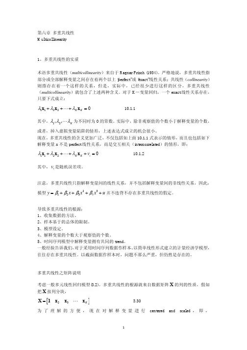
第七章 异方差 Heteroscedasticity1、异方差的实质异方差和自相关是一对,分别检测误差项的方差和协方差,涉及的方法都是GLS 或EGLS 。
同方差的假定如下表示:()221,2,,i E i n εσ== 11.1.1异方差则表示为()22i i E εσ=11.1.22、存在异方差的OLS 估计首先举一个两变量回归模型的例子:异方差下2β的OLS 估计量与同方差假定下的公式(3.1.6)相同,但是它的方差现在由下式给出:()()()22222var ii i x x b x x σ − = −∑∑11.2.2这显然与同方差下的公式3.3.1不同。
()()222var ib x x σ=−∑ (3.3.1) (11.2.3)Proof for 11.2.2.:从一元回归中已知,()()21i i nii x x k x x =−=−∑()2122i i i i i i i b k y k x k ββεβε==++=+∑∑∑()()()()()2222222222211221212112222221122var 22i i n n n n n n n n b E b E k E k k k k k k k E k k k βεεεεεεεεεεε−−=−==++++++=+++∑这是因为无序列相关的假定,误差项交互项乘积的期望等于0。
由于i k 已知,而且()22ii Eεσ=,()()()()()()()222222211222222222211222222222var n n n n i i i i i i i i b k E k E k E k k k k x x x x x x x x εεεσσσσσσ=+++=+++=−−==−−∑∑∑∑∑可以证明在异方差情况下,2b 估计量仍然是线性的和无偏的;同理,不管误差项是否同方差还是异方差,2b 估计量都是一致的估计量;进一步,2b 是asymptotically normally distributed 。
这里关于一元回归在异方差出现下OLS 估计量2b 的特性可以完全推广到多元回归的情况。
但是,在异方差下,2b 虽然是线性、无偏和一致的,却不是有效的和最优的,不具有无偏估计量族中的最小方差。
3、广义最小二乘Generalized Least Squares (GLS)1)广义最小二乘(GLS ) 还是首先回到简单回归模型12i i i y x ββε=++ or ()10201i i i ii y x x x ββε=++=Now assume that the heteroscedasticity variance2i σ are known .012i i i ii i i i y x xεββσσσσ=++11.3.3 For ease of exposition we write as102i i i i y x x ββε∗∗∗∗∗∗=++ 11.3.4where the starred, or transformed, variables are the original variables divided by (the known) i σ.What’s the purpose of transforming the original model?()()2222221var 11i i i i i ii iE E knownεεεσσσσσ∗ ==← == 11.3.5Therefore, the variance of the transformed disturbance term is now homoscedastic.Since we are still retaining the other assumptions of the CLRM, the finding suggest that if we apply OLS to the transformed model 11.3.3 it will produce estimators that are BLUE.This procedure of transforming the original variables in such a way that the transformed variables satisfy the assumptions of the classical model and then applying OLS to them is known as the method of generalized least squares (GLS). In short, GLS is OLS on the transformed variables that satisfy the standard least-squares assumptions. The estimators thus obtained are known as GLS estimators , and it is these estimators that are BLUE.GLS 的估计程序如下:First, we write down the SRF of 11.3.3012ii iii i i i y x x e b b σσσσ∗∗ =++or102i i i i y b x b x e ∗∗∗∗∗∗=++11.3.6Now, to obtain the GLS estimators, we minimize()22102i i i i e y b x b x ∗∗∗∗∗∗=−+∑∑ 11.3.7The actual mechanics of minimizing 11.3.7 follow the standard calculus techniques. The GLS estimator of 2b ∗is()()()()()()()222ii iii ii iii ii iw w x y w x w y bw w x w x ∗−=−∑∑∑∑∑∑∑ 11.3.8 and its variance is given by()()()()222var iii ii iwb w w x w x ∗=−∑∑∑∑ 11.3.9where 21/i i w σ=.2)加权最小二乘(WLS ) Weighted Least Squares (WLS)以简单回归为例。
The unweighted least squares method minimizes2212()iiie y b b x =−−∑∑ 1The weighted least squares minimizes2212()i iiii w e w y bb x ∗∗=−−∑∑2where 12,b b ∗∗are the weighted least-squares estimators 。
In the case of heteroscedasticity, 21i i w σ=, which are inversely proportional to the variance ofi ε or i y .Differencing 2 with respect to 12,b b ∗∗, we obtain()()212121222()12()i i i i i i ii i i i w e w y b b x bw ew y b b x x b ∗∗∗∗∗∗∂=−−−∂∂=−−−∂∑∑∑∑Setting the preceding expressions equal to zero, we obtain the following two normal equations12212i iii ii i ii ii iw y b w b w xw x y b w x b w x∗∗∗∗=+=+∑∑∑∑∑∑Solving these equations simultaneously, we obtain12b y b x ∗∗∗∗=−()()()()()()()222ii iii ii iii ii iw w x y w x w y bw w x w x ∗−=−∑∑∑∑∑∑∑ where /i i i y w y w =∑∑ and /i i i x w x w ∗=∑∑.3)OLS, GLS and WLS总的说来,WLS 只是GLS 的一个特例,但是,在异方差的背景下,GLS 和WLS 术语可以互换;以后我们会讨论GLS 估计的其它特例。
如果确实存在异方差和序列相关性,则通过GLS 这些违背被有效地消除了;如果不存在异方差和序列相关,则GLS 等价于OLS 。
4)矩阵描述GLS 和EGLSTo take into account heteroscedasticity variances (the elements on the main diagonal of 'εε) and autocorrelations in the error terms (the elements off the main diagonal of 'εε), assume that()2'E σ=εεVwhere V is a known n*n matrix. Therefore, if the model is=+y X βεwhere ()0E =ε and ()2var cov σ−=εV . In case 2σ is unknown , which is typically thecase, V then represents the assumed structure of variances and covariances among the random errorsi ε.Under the stated condition of the variance-covariance of the error terms, it can be shown that()1gls 11''−−−=b X V X X V ygls b is known as the generalized least-squares (GLS) estimator of β.It can also be shown that()()1gls21var cov 'σ−−−=bX V XIt can be proved that glsb is the best linear unbiased estimator (BLUE) of β.The real problem in practice is that we do not know 2σ as well as the true variances and covariances (i.e., the structure of the V matrix). As a solution, we can use the method of estimated (or feasible) generalized least squares (EGLS).For EGLS, we first estimate our model by OLS disregarding the problems of heteroscedasticity and/or autocorrelation. We obtaine the residuals from this estimated model and form the(estimated) variance-covariance matrix of the error term, V. It can be shown that EGLS estimators are consisten t estimators of GLS. Symbolically,()111egls''−−−=bX VX X Vy () ()11egls2var cov 'σ−−−=bX V Xwhere Vis an estimate of V .4、异方差下使用OLS 估计的结果假如我们不使用GLS 方法,而是继续使用OLS 方法,我们分别考虑异方差和不考虑异方差两种情况来分析置信区间和假设检验可能出现的不同情况。