劳动经济学第七章
- 格式:ppt
- 大小:131.50 KB
- 文档页数:36










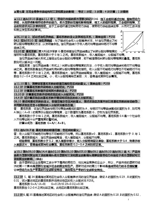
▲第七章不完全竞争市场结构对工资和就业的影响考过1次定;3次简;4次计算;1次案例▲12.1选&07.10多选&11.1定1、劳动力市场的卖方垄断(识记)P246:指工会组织通过控制、限制劳动力供给,从而获得影响劳动条件的能力。
卖方垄断的范围和影响程度,视工人的组织程度、工会组织规模、工会的财政状况以及惯例而定。
由于工会组织通过控制劳动力供给,使劳动力供给曲线左移,从而对工资决定▲06.10论2、试论述洛伦茨曲线、基尼系数的含义及其相互关系。
(简单应用)P25604.1定&07.10定洛伦茨曲线:为了描述社会收入分配差异状况,M·洛伦茨提出了判断分配均等程度的方法,以发明者命名。
洛伦茨曲线介于收入绝对均等曲线和绝对不均等曲线之间。
02.10定基尼系数:意大利经济学家G·基尼根据洛伦茨曲线提出了判断分配均等程度的指标称为基尼系数。
基尼系数介于0与1之间。
基尼系数越大,收入差距越大,分配越不均等。
洛伦茨曲线只能从形式上描绘出社会分配的均等程度,却不能准确地判断分配均等程度的量值。
基尼系数则可以解决这一问题。
相互关系:洛伦茨曲线是(形式上)判断分配均等程度的方法,介于收入绝对均等曲线和绝对不均等曲线之间。
基尼系数是洛伦茨曲线利用判断分配均等程度的指标。
收入分配不可能绝对均等也不可能绝对不均等,基尼系数介于0与1之间。
基尼系数越大,洛伦茨曲线越弯曲,收入差距越大,分配越不均等。
基尼系数在0.2~0.4之间比较正常。
小,收入分配格局缺乏激励;大,容易造成某种社会震荡。
▲11.10简3、简要回答基尼系数的取值范围和各区间的意义。
(简单应用)P25813.1计计算基尼系数并说明收入分配状况。
P25811.1计计算基尼系数值并说明其代表的含义。
P25813.10计计算基尼系数并说明该地区收入分配状况。
P25814.4计试计算该地区的基尼系数并请说明该地区的收入分配状况。
第七章课后答案陈朋辉、李辉工资水平:工资水平是指在单位时期和一定统计范围内劳动者平均工资的数额收入政策:是政府通过非强制性或强制性手段控制工资总水平的政策。
最低工资制度:有关最低工资确立与实施的一系列法律、法令、条例、规定及办法的总称。
包括最低工资法、最低工资标准、实施范围、水平调控及监督手段等内容、它是国家干预用人单位工资水平的一种法定形式。
工资指导线制度:是社会主义市场经济体制下,国家对企业工资分配进行宏观调控的一种制度。
其实施方式为,有关地区结合当年国家对企业工资分配的总体调控目标,综合考虑本地区当年经济增长、物价水平及劳动力市场状况等因素的基础上,提出本地区当年企业工资增长指导意见,企业根据国家的指导意见,在生产发展、经济效益提高的基础上,合理确定本企业当年的工资增长率。
(补充)工资指导线:是在市场经济条件下,政府为保证宏观经济目标的实现,根据社会经济发展相关经济指标的现状与变动,提出的关于年度工资水平增长标准的权威性建议。
工资谈判制度:是指在市场经济条件下,以企业、雇主或其组织为一方,以雇员或工会组织为另一方,双方在政府的指导协调下,就企业工资分配问题进行协商的制度。
劳动负效应补偿性工资差别:有些职业的劳动环境恶劣,给劳动者带来精神损失、健康损失,这种由于“劳动负效应”造成的“非货币损失”需要在工资中给予补偿。
风险补偿性工资差别:有的职业的工资较稳定,有的则变动大;有的职业较稳定有的则不稳定甚至有失业风险,因此,虽然其他条件相同,工资却会有差别,这种差别就成为风险补偿性工资差别。
人力资本补偿性工资差别:人们对人力资本投资是要取得回报的,劳动者进行了教育费用等投资后,在工资上就应有所回报这种对人力资本投资的补偿就在工资上体现出来了。
工资指数化:即通过立法,将工资增长指数与生活费价格指数直接挂钩,定期按照规定的比例自动增加工资。
竞争性工资差别:在劳动力和生产资料可以自由流动的充分竞争条件下,劳动者之间由于本身的劳动效率或劳动技能的差异而形成的工资差别。
《劳动经济学》课后思考题参考答案第一章绪论二、思考题1.如何理解劳动经济学的价值?(1)劳动经济学研究的是社会经济问题。
例如,民工荒、政府要求增加最低工资、劳动生产率下降、农民工工资急剧上升、工资增长不均等、工作培训、国有企业高管人员的高工资受到质疑、收入分配不平、农村移民增加、劳动力市场全球化扩大等等。
(2)数量上的重要性。
在西方经济中,大部分国民收入并不是来源于资本收入(利润、租金和利息),而是来源于工资。
绝大多数居民户的主要收入来源是提供劳务。
从数量上看,劳动才是我们最重要的经济资源。
(3)独有的特性。
劳动力市场的交易完全不同于产品市场的交易。
劳动力市场是一个极有意义和复杂的场所。
劳动力市场的复杂性意味着供给和需求概念在应用于劳动力市场时必须做出重大的修改和调整。
在供给方面,劳动者“出售”给雇主的劳务与该劳动者不可分离。
除了货币报酬,工人还关注工作的健康和安全性、工作难度、就业稳定性、培训和晋升机会等,这类非货币因素也许与直接收入同样重要。
这样,工人的供给决策要比产品市场的供给概念复杂得多。
(4)收益的广泛性。
无论是个人还是社会,都可以从劳动经济学中得到许多启示和教益。
从劳动经济学得到的信息和分析工具有助于人们做出与劳动力市场有关的决策。
从个人角度看。
大量内容将直接与我们有关,如工作搜寻、失业、歧视、工资、劳动力流动等。
对于企业管理者来说,从对劳动经济学的理解中所得到的知识背景和分析方法,对做出有关雇用、解雇、培训和工人报酬等方面的管理决策也应该是十分有用的。
从社会角度看,了解劳动经济学将使人们成为更有知识、更理智的公民。
2.劳动经济学的研究方法有哪些?首先要明确劳动经济学的基本假设。
劳动经济学的假设主要表现在以下四个方面:(1)资源的相对稀缺性。
如同商品和资本是稀缺的一样,劳动力资源也是有限的。
时间、个人收入和社会资源的稀缺性构成了经济学分析的基本前提。
(2)效用最大化。
由于劳动资源的稀缺性,人类社会进行生产经营活动时,必须研究劳动资源的合理配置和利用。
CHAPTER 77-1. Debbie is about to decide which career path to pursue. She has narrowed her options to two alternatives. She can either become a marine biologist or a concert pianist. Debbie lives two periods. In the first, she gets an education. In the second, she works in the labor market. If Debbie becomes a marine biologist, she will spend $15,000 on education in the first period and earn $472,000 in the second period. If she becomes a concert pianist, she will spend $40,000 on education in the first period and then earn $500,000 in the second period.(a) Suppose Debbie can lend and borrow money at a 5 percent annual rate. Which career will she pursue? What if she can lend and borrow money at a 15 percent rate of interest? Will she choose a different option? Why?Debbie will compare the present value of income for each career choice and choose the career with the largest present value. If the discount rate is 5 percent,PV Biologist = – $15,000 + $472,000/(1.05) = $434,523.81andPV Pianist = – $40,000 + $500,000/(1.05) = $436,190.48.Therefore, she will become a pianist. If the rate of interest is 15 percent, however, the present value calculations becomePV Biologist = – $15,000 + $472,000/(1.15) = $395,434.78andPV Pianist = – $40,000 + $500,000/(1.15) = $394,782.61.In this case, Debbie becomes a biologist. As the interest rate increases, the worker discounts future earnings more, lowering the returns from investing in education.(b) Suppose musical conservatories raise their tuition so that it now costs Debbie $60,000 to become a concert pianist. What career will Debbie pursue if the discount rate is 5 percent?Debbie will compare the present value of being a biologist from part (a) with the present value of becoming a pianist. The relevant present values are:PV Biologist = – $15,000 + $472,000/(1.05) = $434,523.81andPV Pianist = – $60,000 + $500,000/(1.05) = $416,190.48.Debbie will, therefore, become a biologist.7-2. Peter lives for three periods. He is currently considering three alternative education-work options. He can start working immediately, earning $100,000 in period 1, $110,000 in period 2 (as his work experience leads to higher productivity), and $90,000 in period 3 (as his skills become obsolete and physical abilities deteriorate). Alternatively, he can spend $50,000 to attend college in period 1 and then earn $180,000 in periods 2 and 3. Finally, he can receive a doctorate degree in period 2 after completing his college education in period 1. This last option will cost him nothing when he is attending graduate school in the second period as his expenses on tuition and books will be covered by a research assistantship. After receiving his doctorate, he will become a professor in a business school and earn $400,000 in period 3. Peter’s discount rate is 20 percent per period. What education path maximizes Peter’s net present value of his lifetime earnings?The present discounted values of Peter’s earnings associated with each of the alternatives are167,254$2.1000,902.1000,110000,1002=++=HS PV , 000,225$2.1000,1802.1000,180000,502=++−=COL PV , and 778,227$2.1000,4002.10000,502=++−=PhD PV .Thus, the best option for Peter is to start working upon completely high school.7-3. Jane has three years of college, Pam has two, and Mary has one. Jane earns $21 per hour, Pam earns $19, and Mary earns $16. The difference in educational attainment is due completely to different discount rates. How much can the available information reveal about each woman’s discount rate?The returns to increasing one’s education from one to two years of college and then from two to three years of college are%75.1816$16$19$21=−=to r and %53.1019$19$21$32=−=to r .Having observed their educational choices, we know that Mary’s discount rate is greater than 18.75 percent, Pam’s is between 10.53 percent and 18.75 percent, and Jane’s is less than 10.53 percent.7-4. Suppose the skills acquired in school depreciate over time, perhaps because technologicalchange makes the things learned in school obsolete. What happens to a worker’s optimal amount of schooling if the rate of depreciation increases?If the rate of depreciation is very high, the payoff to educational investments declines. As a result, a worker’s optimal amount of schooling will also fall as the benefits of education erode rapidly.7-5. Suppose workers differ in their ability, but have the same discount rate. Is it possible for the more able workers to choose less schooling?This result is possible as long as more able workers have lower marginal-rate-of-discount curves. For example, if an 18-year-old basketball player can earn $3 million per year by entering the NBA after high school whereas he would earn $3.25 million per year by entering the NBA after college, the opportunity cost of college ($3 million per year) may be so great that the player opts to skip college. (A similar story might explain why Bill Gates dropped out of Harvard.)7-6. Suppose Carl’s wage-schooling locus is given byYears of Schooling Earnings6 $10,0007 $12,8008 $16,0009 $18,50010 $20,35011 $22,00012 $23,10013 $23,90014 $24,000(a) Derive the marginal rate of return schedule. When will Carl quit school if his discount rate is 4 percent? What if the discount rate is 12 percent?The marginal rate of return is given by the percentage increase in earnings if the worker goes to school one additional year.Schooling Earnings MRR6 $10,00028.07 $12,80025.08 $16,0009 $18,50015.610 $20,350 10.011 $22,000 8.112 $23,100 5.013 $23,900 3.514 $24,000 0.4Carl will quit school when the marginal rate of return to schooling falls below his discount rate. If his discount rate is 4 percent, therefore, he will quit after 12 years of schooling; if his discount rate is 12 percent, he will quit after 9 years of schooling.(b) Suppose the government imposes an income tax of 20 percent on both labor earnings and interest income. What is the effect of this income tax on Carl’s educational attainment?This is a tricky problem. If Carl is making his educational decision by comparing the marginal rate of return to schooling to some rate of discount that does not depend on the government’s tax policies, then it turns out that Carl’s optimal schooling level is unchanged. It is easy to verify that if the governmentimposes a 20 percent tax rate on labor earnings in the second column of the table above, the marginal rate of return to schooling (column 3) remains unchanged. If, however, Carl’s rate of discount is affected by the government’s tax policies (for example, Carl’s rate of discount might be affected by the rate of interest banks pay), then Carl’s educational decision will be affected. For example, if Carl’s rate of discount falls by 20 percent then the amount of schooling acquired goes up because the marginal rate of return schedule in column 3 of the table has changed.7-7. In the typical signaling model, it is assumed that the costs of acquiring an education are higher for low-ability than for high-ability workers. Suppose the government subsidizes low-ability workers for the higher costs they incur in obtaining an education. What happens to the signaling value of education? Can there be a perfectly separating equilibrium in this labor market?If the government subsidizes schooling so that the cost of schooling is the same for all workers, then the signaling value of schooling is lost. There cannot be a perfectly separating equilibrium because all workers would have the same incentive to obtain the same amount of schooling.7-8. Suppose there are two types of persons: high-ability and low-ability. A particular diploma costs a high-ability person $8,000 and costs a low-ability person $20,000. Firms wish to use education as a screening device where they intend to pay $25,000 to workers without a diploma and $K to those with a diploma. In what range must K be to make this an effective screening device?In order for a low-ability worker to not pursue education, it must be that $25,000 ≥K – $20,000 which requires K≤ $45,000. Similarly, in order for a high-ability worker to pursue education, it must be that K – $8,000 ≥ $25,000 which requires K≥ $33,000. Thus, in order to use education as a signaling device, it must be that educated workers are paid between $33,000 and $45,000.7-9. It has been argued that the minimum wage prevents workers from investing in on-the-job training and discourages employers from providing specific training to low-income workers. Why would the minimum wage have an adverse effect on human capital accumulation for low-income workers?First, when the minimum wage is high, the marginal return to on-the-job investment falls (assuming one can always find a job), and therefore the lowest skill workers may no longer find it useful to engage in on-the-job training.Second, a firm that offers general or specific training in the first period pays the worker a wage below his or her marginal product while the investment is taking place and above his or her marginal product in the post-investment period. If the minimum wage prevents the investment-period wage from falling sufficiently, however, firms may not be able to offer the training.7-10. Jill is planning the timing of her on-the-job training investments over the life cycle. What happens to Jill’s OJT investments at every age if(a) the market-determined rental rate to an efficiency unit falls?The marginal revenue of investing in OJT declines so that Jill will invest less at each age.(b) Jill’s discount rate increases?If Jill’s discount rate increases she becomes more “present oriented”, reducing the future benefits associated with OJT. Thus her OJT investments fall.(c) the government passes legislation delaying the retirement age until age 70.The marginal revenue of investing in OJT increases because the payoff period to the investment is longer. Thus, she undertakes more OJT in this case.(d) technological progress is such that much of the OJT acquired at any given age becomes obsolete within the next 10 years.The marginal revenue to investing in OJT declines and the amount of OJT acquired falls.7-11. In 2000, there were about 9 million students in four-year college institutions in the United States. Believing that education is the key to the future, a presidential candidate proposes that the federal government pay the first $3,000 of college expenses each year for everyone attending a four-year college. It is expected that this proposal will encourage 3 million more people to enroll in a four-year college each year, but that the graduation rate will fall from 80 percent to 75 percent. What is the yearly projected cost of the program? What is the average cost of the plan per new student attending a four-year college? What is the average cost of each new four-year college graduate?Under the old plan, 9 million students attended a four-year college each year, with 80 percent (7.2 million) eventually graduating. Under the new plan, 12 million students will attend a four-year college each year, with 75 percent (9 million) eventually graduating. The annual cost of the program, therefore, is 12 million × $3,000 = $36 billion. The average cost of the plan per new college student is $36b / 3m = $12,000. The average cost of each new graduate is $36b / 1.8m = $20,000.7-12. In 1970, men aged 18 to 25 were subject to the military draft to serve in the Vietnam War. A man could qualify for a student deferment, however, if he was enrolled in college and made satisfactory progress on obtaining a degree. By 1975, the draft was no longer in existence. The draft did not pertain to women. Using the data in Table 255 of the 2002 edition of the U.S. Statistical Abstract, use women as the control group to estimate (using the difference-in-differences methodology) the effect abolishing the draft had on male college enrollment.The difference-in-differences table isCollege Enrollment (percentage)Diff-in-diff1970 1975 DiffMen 55.2 52.6 -2.6 -3.1Women 48.5 49.0 0.5Thus, abolishing the draft is estimated to lower the college enrollment rate of men by 3.1 percentage points.。