分子动力学模拟基础知识
- 格式:pdf
- 大小:1.05 MB
- 文档页数:42
分子模拟基础知识点总结1. 分子力场分子力场是分子模拟的基础,它描述了分子内部原子之间的相互作用力。
分子力场通常包括键的形成和断裂、原子间的相互作用力(如范德瓦尔斯力和静电相互作用力)等。
分子力场模型是根据实验数据和理论计算结果来拟合的,常见的分子力场模型包括AMBER、CHARMM、OPLS等。
分子力场模型的好坏直接影响了分子模拟的结果,因此选择合适的分子力场模型是非常重要的。
2. 分子动力学分子动力学是一种模拟分子在封闭系统中随时间演化的方法。
分子动力学通过求解牛顿运动方程,推导出分子在力场作用下的位移、速度和加速度,从而获得分子的运动轨迹和动力学性质。
分子动力学模拟的关键是要确定分子的初态,即分子的初始位置和速度分布,通过数值积分的方法,可以计算出分子在任意时刻的位置和速度。
分子动力学在研究分子或材料的结构、动力学行为和热力学性质方面有广泛的应用。
3. 蒙特卡洛模拟蒙特卡洛模拟是一种以随机抽样的方法对系统进行模拟的方法。
在蒙特卡洛模拟中,系统中的每一个粒子都有一定的概率发生随机运动,从而使得系统的状态随时间发生变化。
蒙特卡洛模拟通常用于模拟体系的平衡态性质,如热力学性质和相平衡等。
蒙特卡洛模拟的关键是要设计合适的随机抽样方法,并通过大量的模拟样本来获得系统的统计性质。
4. 分子模拟在材料科学中的应用在材料科学中,分子模拟被广泛应用于研究材料的结构、力学性质、热电性质、传输性质等。
通过分子模拟,可以预测材料的力学性质(如弹性模量、屈服强度等)、热电性质(如热导率、热膨胀系数等)、传输性质(如扩散系数、电导率等)等。
分子模拟还可以帮助设计新型的材料,并优化材料的性能。
5. 分子模拟在生物科学中的应用在生物科学中,分子模拟被广泛应用于研究生物分子的结构、功能和相互作用。
通过分子模拟,可以预测蛋白质的结构、预测蛋白质-配体和蛋白质-蛋白质的相互作用方式,从而为药物设计和药物筛选提供理论依据。
分子模拟还可以研究细胞膜的结构和功能,预测药物分子的跨膜转运方式等。

生物物理学中的分子动力学模拟生物物理学是生物学与物理学的交叉学科,旨在研究生物大分子的结构与功能。
分子动力学模拟是生物物理学中的重要工具,用于研究分子在不同环境下的动力学行为。
本文将介绍分子动力学模拟的基本概念、应用和未来发展方向。
一、分子动力学模拟基本概念分子动力学模拟是利用计算机模拟分子在经典牛顿力学下的运动轨迹的过程。
分子动力学模拟的基本思想是将分子看作一组球体,通过求解牛顿运动方程,模拟它们在空间中的运动轨迹。
在模拟过程中,通过设置合适的势函数来描述分子之间的相互作用。
势函数主要包括键能、库伦势、范德华力、电子偶极子相互作用等。
模拟过程中还需要考虑分子的初始构象、温度、压力和场强等因素的影响。
二、分子动力学模拟的应用分子动力学模拟在生物物理学中的应用非常广泛,以下是一些常见的应用:1. 蛋白质动力学模拟蛋白质是生命体系中最重要的大分子之一,其结构与功能密切相关。
通过蛋白质动力学模拟,可以研究蛋白质的构象变化、动态行为及其与其他分子之间的相互作用。
例如,在研究药物靶点时,可以通过模拟药物分子与靶点蛋白之间的相互作用,来预测药物的活性及其副作用。
2. 生物膜模拟生物膜是生物体内各种细胞和细胞器之间的界面结构,是细胞膜的重要组成部分。
生物膜由脂质分子和蛋白质构成,其特殊的物理化学特性使得模拟其行为是非常具有挑战性的。
通过模拟生物膜的形成和变化,可以研究生物分子在膜内的运动与相互作用,为疾病治疗等领域提供理论基础。
3. RNA模拟RNA与DNA一样都是核酸分子,但其在功能和结构上有着巨大的差异。
通过RNA分子的模拟,可以研究RNA的三维结构、相互作用和在转录和翻译过程中的生物学功能等方面的问题,为生物医药领域的研究提供重要支撑。
三、分子动力学模拟的未来发展方向分子动力学模拟的应用领域不断扩大,未来其在生物物理学领域的应用将更为广泛。
以下是一些未来的发展方向:1. 强化学习算法在模拟中的应用强化学习是一种机器学习方法,在分子动力学模拟中,可以将其应用于动力学过程的控制和优化。
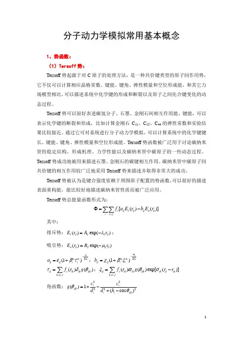
分子动力学模拟常用基本概念1、势函数: (1)Tersoff 势:Tersoff 势起源于对C 原子的处理方法,是一种共价键类型的原子间作用势,它不仅可以计算相应晶格常数、键能、键角、弹性模量和空位形成能,和其它力场模型相比,可以描述系统中化学键的形成和断裂以及原子之间化合键变化的动态过程。
Tersoff 势可以很好表述碳氢分子、石墨、金刚石间相互作用能、键能,可以表示化学键的断裂和形成,比如计算金刚石C 11、C 12、C 44的弹性常数和实验结果比较接近。
通过它可对系统进行分子动力学模拟,可以计算系统中的化学键键长、键能、键角、弹性模量和空位形成能。
Tersoff 势函数被广泛用于讨论碳纳米管的稳定结构、形成机理、力学性能以及碳纳米管中碳原子的一些动态过程。
Tersoff 势成功地被用来描述石墨、金刚石的碳键相互作用。
碳纳米管中碳原子间共价键的相互作用较广泛地采用Tersoff 势来描述并取得非常大的成功。
Tersoff 势被认为是键合强度依赖于周围原子配置的势函数,可以很好的描述表面重构能,能比较好地描述碳纳米管性质而被广泛应用。
Tersoff 势总能量函数形式为:[()()]c ij r ij ij a ij ii jf a E r b E r <Φ=-∑∑其中:排斥势:()exp()r ij ij ij ij E r A r λ=-; 吸引势:()exp()a ij ij ij ij E r B r μ=-12(1)i i innn ij ij i i a εβτ-=+;2(1)i iiim n nn ij ij i i b χβξ-=+,()()ij c ik ik ijk k i jf rg τδθ≠=∑;,()()exp[()]ij c ik ik ijk ik ij ik k i jf rg r r ξϖθσ≠=-∑角函数:22222()1(cos )iiijk ii i ijk c c g d d h θθ=+-+-截断函数:11()[1cos()]20ij ij c ik ij ijr R f r S R π⎧⎪-⎪=+⎨-⎪⎪⎩式中,αij 是截断距离,一般情况下,必须将αij 式中的β的值取得充分小,使得αij ≈1,因为在第一临近之外的范围内,τij 会指数式地变大。
分子动力学模拟(二)引言概述:分子动力学模拟是一种通过模拟分子之间相互作用力和相对位置的方法,来研究系统在不同条件下的动力学行为的技术。
本文将继续探讨分子动力学模拟的应用领域并深入介绍其在材料科学、生物医学和化学等领域的具体应用。
一、材料科学中的分子动力学模拟1. 分子结构与性质的研究1.1 分子间相互作用力的模拟与计算1.2 晶体缺陷与物理性质的关联1.3 材料相变的模拟及驱动机制的研究1.4 纳米材料的热力学性质模拟1.5 材料表面与界面的模拟研究2. 材料设计与优化2.1 基于分子动力学模拟的材料设计方法2.2 优化材料的结构与性能2.3 基于计算的高通量材料筛选2.4 分子动力学模拟在材料工程中的应用案例2.5 材料仿真与实验的结合二、生物医学中的分子动力学模拟1. 蛋白质结构与功能的研究1.1 蛋白质折叠和构象转变的模拟1.2 水溶液中蛋白质的动力学行为1.3 药物与蛋白质的相互作用模拟1.4 多肽和蛋白质的动态模拟1.5 分子动力学模拟在药物设计中的应用2. 病毒与细胞相互作用的模拟2.1 病毒与宿主细胞的相互识别与结合2.2 病毒感染过程的动态模拟2.3 细胞信号传导的分子动力学模拟2.4 细胞内各组分的动态行为模拟2.5 分子动力学模拟在生物药物研发中的应用三、化学中的分子动力学模拟1. 化学反应的机理研究1.1 反应路径与转变态的模拟1.2 温度和压力对反应速率的影响1.3 催化反应的模拟与优化1.4 化学反应中的动态效应模拟1.5 化学反应机理的解析与预测2. 溶液中的分子行为模拟2.1 溶剂效应的模拟与计算2.2 溶液中的分子运动与扩散2.3 溶液界面的分子动力学模拟2.4 溶液中的化学平衡与反应行为2.5 分子动力学模拟在化学合成与设计中的应用总结:分子动力学模拟在材料科学、生物医学和化学等领域具有广泛的应用前景。
通过模拟分子间交互作用力和相对位置的变化,可以深入研究分子系统的动力学行为,为材料设计、药物研发和化学反应机理的解析提供重要参考。

分子动力学模拟实验的原理与方法一、引言分子动力学模拟实验是一种基于分子运动规律的计算方法,通过模拟分子间相互作用力和运动轨迹,可以研究物质的结构、性质和动力学过程。
本文将介绍分子动力学模拟实验的原理与方法,包括模拟算法、模拟体系的构建和模拟结果的分析。
二、分子动力学模拟的原理分子动力学模拟实验基于牛顿力学和统计力学的原理,通过求解分子系统的运动方程,模拟分子间相互作用力和运动轨迹。
其基本原理可以概括为以下几点:1. 分子运动方程分子动力学模拟实验中,每个分子都被看作是一个质点,其运动方程可以由牛顿第二定律得到。
根据分子的质量、受力和加速度,可以得到分子的位置和速度随时间的变化。
2. 分子间相互作用力分子间的相互作用力可以通过势能函数来描述,常见的势能函数包括Lennard-Jones势和Coulomb势。
这些势能函数描述了分子间的吸引力和排斥力,从而影响分子的相互作用和运动。
3. 温度和压力控制分子动力学模拟实验中,为了模拟实际系统的温度和压力条件,需要引入温度和压力控制算法。
常见的温度控制算法包括Berendsen热浴算法和Nosé-Hoover热浴算法,压力控制算法包括Berendsen压力控制算法和Parrinello-Rahman压力控制算法。
三、分子动力学模拟的方法分子动力学模拟实验的方法包括模拟算法、模拟体系的构建和模拟结果的分析。
下面将对这些方法进行介绍。
1. 模拟算法分子动力学模拟实验中,常用的模拟算法包括经典力场方法和量子力场方法。
经典力场方法基于经验势能函数,适用于大尺度的分子系统,如蛋白质和溶液。
量子力场方法基于量子力学原理,适用于小尺度的分子系统,如分子反应和电子结构计算。
2. 模拟体系的构建模拟体系的构建是分子动力学模拟实验中的重要步骤,包括选择模拟系统、确定初始结构和参数设置。
模拟系统的选择应根据研究的目的和问题,可以是单个分子、溶液系统或固体表面。
初始结构可以通过实验数据、计算方法或模型生成,参数设置包括力场参数、温度和压力等。

计算机模拟分子动力学的理论和方法计算机模拟分子动力学是一种拟合物理实验和理论计算的分子动力学模拟方法。
它通过在计算机上模拟分子的运动来研究分子结构和相互作用,从而探索分子力学和统计物理学。
从宏观上看,这种方法能更好的了解不同分子之间的作用力和反应,以推测分子之间的物理特征,是一种十分有效的分子结构解析办法。
本文将详细介绍计算机模拟分子动力学的理论和方法。
1.分子动力学的理论基础分子动力学的理论基础是牛顿经典力学原理和统计力学。
它假定分子是一个粒子固体,分子之间的相互作用可以表示为势能函数。
分子之间的相互作用被分解为键角位与复杂的杂化力项。
通过牛顿方程和势能函数对分子的运动进行计算,可以得到分子的相关参数如位移,速度,绘图等,以了解分子的微观特征。
2.计算机模拟分子动力学的方法计算机模拟分子动力学的方法是通过计算机程序模拟分子运动状态。
首先,需要在计算机上特定的仿真软件及数据分析工具,设置分子模型、化学键强弱参数。
接着,设定一定的仿真条件,并通过一定的计算方法生成分子动力学模型。
然后,通过处理数据获得更多的物理信息或大型运行里程。
3.计算机模拟分子动力学的应用计算机模拟分子动力学应用十分广泛。
它可以被用来研究分子之间的相互作用,探索分子的物理特征,从而探究和预测分子对其他物质和环境的响应。
例如,它可以用来探索药物研究、金属熔化和凝聚、聚合物物理等方面。
此外,计算机模拟分子动力学在材料物理学和生命科学中的潜力非常巨大。
总的来说,计算机模拟分子动力学是目前分子动力学研究领域中的一项重要技术。
它融合了物理、化学、计算机科学等多学科技术,为人们对分子特性和作用力的进一步探究提供了有效工具。
尽管它在一定程度上依赖于计算机处理力的提升,但随着计算机科学与技术的不断进步,计算机模拟分子动力学在分子科学研究中的地位将会变得更为重要。
引言概述:分子动力学模拟(MD)是一种模拟系统内原子或分子运动的计算方法,通过计算原子之间的相互作用力和运动方程,可以研究材料的物理和化学性质、相互作用和动态行为等。
本文将深入探讨分子动力学模拟的相关内容,包括模拟算法、分子模型构建、初始条件设定、系统参数调优、结果分析等。
正文内容:一、模拟算法1.1简单分子动力学模拟算法:介绍经典分子动力学模拟的基本原理和算法。
1.2高级模拟算法:介绍一些基于统计力学和量子力学原理的高级分子动力学模拟算法,如MonteCarlo方法和量子分子动力学模拟。
二、分子模型构建2.1原子选择:根据研究对象和目的,选择适合的原子种类。
2.2原子间相互作用模型:介绍常用的原子间相互作用势函数模型,如LennardJones势和Coulomb势等。
2.3拓扑构建:说明如何根据分子结构构建拓扑,包括原子连接方式和键长、键角、二面角等参数。
三、初始条件设定3.1初始构型:介绍如何原子或分子的初始位置和速度。
3.2温度控制:讨论如何在模拟中控制温度,包括使用温度计算公式和应用恒温算法等。
3.3压力控制:介绍如何在模拟中控制压力,包括应用压力计算公式和应用恒压算法等。
四、系统参数调优4.1时间步长选择:讲解如何选择合适的时间步长,以确保模拟结果的准确性和稳定性。
4.2模拟时间长度:介绍如何选取适当的模拟时间长度,以获得足够的统计样本。
4.3系统尺寸选择:探讨系统尺寸对模拟结果的影响,包括边界条件的选择和静电相互作用的处理。
五、结果分析5.1动力学参数计算:介绍如何通过模拟数据计算动力学参数,包括径向分布函数和速度自相关函数等。
5.2结构参数分析:讨论如何分析模拟结果中的结构特征,如配位数、键长分布和角度分布等。
5.3物理性质计算:讲解如何通过模拟数据计算材料的物理性质,如热力学性质和动力学性质等。
总结:分子动力学模拟是一种强大的计算工具,可以模拟和研究材料的动态行为和性质。
从模拟算法、分子模型构建、初始条件设定、系统参数调优到结果分析,每个步骤都需要仔细考虑和调整,以保证模拟结果的准确性和可靠性。

分子动力学模拟的若干基础应用和理论一、本文概述分子动力学模拟是一种基于经典力学的计算方法,通过求解分子体系的牛顿运动方程,模拟分子在特定条件下的动态行为。
该方法广泛应用于物理、化学、生物和材料科学等领域,为研究者提供了一种有效的工具,以深入理解和预测分子系统的宏观性质。
本文旨在探讨分子动力学模拟的若干基础应用和理论,从基础概念出发,阐述其基本原理、模拟方法以及在各个领域中的应用实例。
我们将详细介绍分子动力学模拟的核心技术,包括力场模型、初始条件设定、积分算法和模拟结果的解析等。
本文还将讨论分子动力学模拟的局限性以及未来的发展方向,以期为相关领域的研究人员提供有益的参考和启示。
二、分子动力学模拟的理论基础分子动力学模拟(Molecular Dynamics Simulation, MDS)是一种强大的计算技术,通过求解分子体系的牛顿运动方程,模拟分子在特定条件下的动态行为。
其理论基础主要建立在经典力学、统计力学以及量子力学之上,但在大多数应用中,由于计算能力的限制,经典力学是主要的工具。
在经典力学中,每个分子的运动可以通过牛顿第二定律来描述,即力等于质量乘以加速度(F=ma)。
在分子动力学中,这些力通常是分子间相互作用力,包括范德华力、氢键、库仑力等。
这些力可以通过分子力学模型或量子力学方法计算得出。
分子动力学模拟通常包括以下几个主要步骤:需要设定模拟的初始条件,包括分子的初始位置、速度和模拟的温度、压力等环境参数。
然后,根据分子间的相互作用力,通过求解牛顿运动方程,计算出每个分子在下一时刻的位置和速度。
这个过程会不断重复,直到模拟达到预设的时间长度或达到某种平衡状态。
在模拟过程中,为了处理大量的分子和长时间的模拟,通常会采用一些近似和简化的方法,如截断半径、周期性边界条件等。
由于分子间的相互作用力往往非常复杂,因此在模拟中通常会采用一些经验性的力场模型,如Lennard-Jones势、Morse势等。

分子动力学模拟的原理及其应用随着计算机技术的高速发展,分子动力学模拟(Molecular Dynamics Simulation,MD)已经成为了一种重要的理论与计算方法,在化学、物理、材料、生物等领域得到了广泛的应用。
其主要基于牛顿第二定律,通过数值计算来模拟分子的运动,从而揭示分子间的相互作用、热力学性质等信息。
一、分子动力学模拟的基本原理分子动力学模拟是一种建立在分子间相互作用的基础上,通过解牛顿方程的计算方法,模拟分子的运动行为的一种理论与计算方法。
(一)牛顿第二定律牛顿第二定律描述了物体所受合外力作用时的加速度和质量之间的关系。
对于一个质量为m的物体,它的加速度a和作用力F 之间的关系为:F=ma。
(二)化学键势能对于一个化学体系,其所具有的能量主要由势能、动能以及相互作用能组成。
其中,化学键势能是用来反映原子间距离、化学键的力常数等因素的有效能量。
(三)Newton运动方程Newton运动方程描述了物体在给定的力学场中的运动状态,即物体在时间t内的速度、位移和加速度的关系。
对于一个单分子的系统来说,其牛顿运动方程可以被表示为:F=ma其中,F为作用于原子i的外力,m为原子i的质量,a为原子i 的加速度。
(四)Verlet算法提出了用于原子振动的时间推进算法,被称为Verlet算法。
在这种算法中,通过使用当前时间步长、前一个时间步长和后一个时间步长的位置(在时间段内)来估计当前时间步长的速度。
在迭代计算中,原子的加速度取决于位置和能量的二阶导数。
二、分子动力学模拟的应用领域分子动力学模拟已经广泛应用于化学、物理、材料、生命科学与生物技术等领域,其中包括:(一)材料科学MD可以被用来模拟材料中的原子运动行为,这些材料可以包括分子、聚合物、合金、晶体、液晶等。
(二)生命科学MD可以用来研究生物大分子,如蛋白质结构和功能,核酸的结构和动力学,以及膜蛋白等的结构和功能。
其还可以用于药物的发现与设计。

分子动力学模拟的理论与实践分子动力学模拟(Molecular Dynamics,MD)是计算物理领域中的一种重要方法,可以用来模拟大量分子间的相互作用、动力学和结构性质。
它是一种基于牛顿力学和量子力学的计算方法,能够模拟不同温度和压力下的物质性质,达到预测性能的效果。
分子动力学模拟的理论基础分子动力学模拟的基础理论是基于牛顿运动定律和量子力学的分子的波动方程。
在这个系统中,每个分子都可以等效地表示为一个三维空间中的点粒子,其在每个时刻都可能受到其他周围分子的作用力而产生运动。
这个过程的变化可以用波动方程来描述,通过数值方法进行求解。
从数学上说,MD模拟中每个时刻都被表示为一个离散的时间步长,其大小通常为数飞秒到数千飞秒不等。
在每个时间步长内,通过牛顿定律计算每个分子的加速度和位置,从而确定下一个时刻的分子位置和运动状态。
分子动力学模拟的实际应用由于分子动力学模拟的高仿真性,在材料、药物研究,纳米材料设计等领域,已经得到了广泛地应用。
例如,在纳米材料中,MD模拟可以帮助研究人员更好地理解材料性质、预测相关性能和缺陷,从而提高设计和生产效率。
在药物研究中,MD模拟可以用来开发新的药物分子,评估其潜在活性,并为进一步研究疾病机理提供可靠的平台。
分子动力学模拟也被广泛应用于材料损伤和断裂研究。
在这个领域,MD模拟可以模拟材料中分子的相互作用,研究材料容限和断口扩展的性质和机制,从而为新材料设计和制造提供技术支持。
对分子动力学模拟的进一步发展的展望尽管分子动力学模拟已经在许多应用中显著地证明了其性能,但仍然存在许多挑战,包括模拟许多分子的复杂性,以及不同分子相互作用之间的复杂性。
未来,开发更高效的数值方法可以帮助克服这些限制,而更好的分子力场模型和算法设计可以提高模拟结果的准确性和预测性能。
此外,利用高性能密集型计算设备和更先进的并行计算技术也可以进一步加快分子动力学模拟的计算速度。
总之,随着计算机技术的迅猛发展,分子动力学模拟的应用将更加广泛,也会不断地更新和发展其方法和技术。
分子动力学模拟分子动力学模拟:解开分子世界的奥秘分子动力学模拟是一种模拟分子间相互作用和运动的计算方法,利用数学算法和计算机模拟技术,可以研究原子和分子的行为。
它已经成为物理学、化学、生物学等领域研究中不可或缺的工具。
本文将介绍分子动力学模拟的原理、应用以及未来发展方向。
一、分子动力学模拟的基本原理分子动力学模拟是基于牛顿力学和统计力学的基本原理进行的。
它假设分子是由原子构成的,每个原子受到的势能和力可以通过计算得到。
通过计算分子系统中的粒子的速度和位置,可以模拟其运动和变化。
模拟过程中,使用时间步长将时间分割为很小的片段,通过求解经典牛顿定律方程的数值解来模拟粒子在力场中的运动。
二、分子动力学模拟的应用领域1. 材料科学领域分子动力学模拟在材料科学中有着广泛的应用。
通过模拟不同条件下原子和分子的运动,可以探究材料的结构、力学性质、热学性质等。
例如,可用于研究材料的疲劳性能、塑性变形机制以及材料的断裂行为等。
通过对材料的分子动力学模拟,可以对材料的特性进行预测和优化,为材料设计和制造提供指导。
2. 生物科学领域分子动力学模拟在生物科学领域的应用也非常广泛。
可以将分子动力学模拟应用于药物设计中,通过模拟药物与受体之间的相互作用,预测药物在生物体内的活性和选择性。
此外,分子动力学模拟还可以用于研究蛋白质的折叠机理、蛋白质-核酸相互作用等生物过程,以及研究细胞膜对物质的输运和分析等。
三、分子动力学模拟的挑战和未来发展方向虽然分子动力学模拟在理论和应用上取得了显著进展,但仍然面临一些挑战。
首先,大规模系统的模拟需要耗费大量的计算资源和时间,限制了研究的扩展性。
其次,精确描述原子与分子之间的相互作用仍然是一个困难的问题,当前的力场模型和参数化方法仍有提升空间。
此外,由于分子动力学模拟是一个数值计算方法,误差的累计可能导致模拟的不准确性。
因此,提高计算精度和效率仍然是未来发展的方向。
未来的发展方向之一是结合机器学习和深度学习等人工智能技术,将其应用于分子动力学模拟中。
分子动力学模拟方法及应用概述分子动力学模拟是一种基于牛顿力学原理和统计力学的计算模拟方法,可用于研究物质的微观结构和动力学行为。
本文将介绍分子动力学模拟的基本原理和常用的计算方法,以及它在不同领域的应用。
一、分子动力学模拟的基本原理分子动力学模拟基于经典力学理论,通过求解牛顿运动方程来模拟物质的运动行为。
它假设系统中的分子为硬球或软球,根据分子之间的相互作用力、动能和位能,计算分子的运动轨迹和力学性质。
1. 分子间相互作用力分子间的相互作用力主要包括范德华力、静电力和键能。
范德华力描述非极性分子之间的相互作用力,静电力描述电荷之间的相互作用力,而键能则表示化学键的形成和断裂过程。
这些相互作用力的计算对于准确模拟分子的行为至关重要。
2. 动力学方程分子动力学模拟基于牛顿第二定律,即F=ma。
其中,F 是分子所受的合外力,m是分子的质量,a是加速度。
通过求解这些动力学方程,可以得到分子的位置和速度随时间的演化。
二、常用的分子动力学模拟方法在分子动力学模拟中,为了准确模拟系统行为,需要借助适当的计算方法和技术。
以下是几种常用的分子动力学模拟方法。
1. Verlet算法Verlet算法是最常用的求解分子动力学方程的方法之一。
它基于泰勒级数展开,通过利用前一时刻的位置和加速度来预测当前时刻的位置。
Verlet算法具有较高的计算精度和稳定性。
2. Monte Carlo模拟除了分子动力学模拟,Monte Carlo模拟也是一种常用的计算方法。
它基于随机抽样的方法,通过模拟系统的状态转移来研究系统的平衡性质和统计性质。
Monte Carlo模拟在研究液体和固体的相变、化学反应等方面具有重要的应用。
3. 并行计算由于分子动力学模拟的计算复杂性很高,为了提高计算效率,通常需要借助并行计算技术。
并行计算可以将任务分配给多个处理器或计算节点进行并行计算,大大提高了计算速度和效率。
三、分子动力学模拟的应用领域分子动力学模拟在化学、材料科学、生物物理学等领域具有广泛的应用。
化学中的分子动力学模拟方法分子动力学模拟是一种重要的计算方法,主要用于研究分子的运动和相互作用,可以用于探究分子间的各种特性和反应。
一、分子动力学模拟的基本原理分子动力学模拟基于牛顿力学原理,将分子看作由粒子组成的系统,通过计算运动粒子之间的相互作用能量和力的大小方向,来预测粒子运动的轨迹和系统的特性。
在分子动力学模拟中,通常采用科学计算软件进行计算,模拟计算的精度和效率受到计算机处理能力和理论模型的限制。
二、分子动力学模拟的应用分子动力学模拟在化学、生物、材料科学等领域应用广泛,可以用于设计新材料、药物开发、酶催化机理、晶体生长等研究。
下面就是几个具体的应用案例:1. 材料表征分子动力学模拟可以通过模拟材料的原子运动来研究材料的动力学性质、热力学性质和机械性质。
在材料表征方面,分子动力学模拟可以用于研究熔化、固化、晶化等过程。
2. 催化研究分子动力学模拟可以用于研究化学反应的催化机理和反应动力学,例如在催化剂表面上反应的机理和吸附方式等。
这些研究对于催化反应速率和产物选择性的理解非常重要。
3. 蛋白质研究分子动力学模拟可以用于研究蛋白质的结构、动力学、功能和相互作用。
例如,分子动力学模拟可以用于研究酶催化机理、蛋白质配体作用和蛋白质构象变化。
4. 药物研究分子动力学模拟可以用于研究化合物与生物分子的相互作用,从而预测药物分子的结合模式和选通性。
分子动力学模拟可以用于设计新的药物分子,改善已有分子的活性和特异性。
三、分子动力学模拟中的算法和计算效率分子动力学模拟中的算法可以分为多种,如Verlet算法、Leapfrog算法、Runge-Kutta算法等。
不同算法的精度和计算复杂度不同,选用适当的算法可以提高计算效率和准确度。
分子动力学模拟的计算时间也是一个重要的因素。
由于分子动力学模拟涉及到大量的原子和分子运动,计算复杂度较高。
因此,现代计算机科学在此方面发挥了重要的作用,如并行计算、GPU加速等技术,使得分子动力学模拟的计算效率得到了很大提升。
分子动力学基础知识点总结分子动力学的基础知识点主要包括以下几个方面:1. 分子结构和动力学描述分子是由原子构成的,原子之间通过化学键相连形成分子。
分子的结构对其在空间中的运动和相互作用产生很大影响。
分子动力学通过分子结构的描述和分子运动的模拟,探讨分子之间的相互作用力和分子在各种条件下的动力学行为。
2. 分子间相互作用力分子间相互作用力是分子动力学研究的重要内容。
分子之间的相互作用受到范德华力、静电力、氢键等多种因素的影响。
这些相互作用力决定了分子的结构稳定性、化学反应速率和物质的性质等方面。
3. 分子的运动分子的运动是分子动力学研究的核心内容之一。
分子在空间中以不同的方式运动,包括平动、转动和振动。
这些运动形式对物质的热学性质、力学性质和光学性质都有着重要影响。
4. 孤立分子和聚集态分子的动力学分子动力学可以研究孤立分子和聚集态分子在不同条件下的动力学行为。
孤立分子通常在热学激发或高能激发下进行各种运动,而聚集态分子在液态或固态条件下则受到相互作用力的影响,部分分子之间通过相互作用形成新的结构和性质。
5. 分子运动和材料性质的关系分子动力学的研究对于材料科学有着重要意义。
分子在材料中的运动和相互作用形成了材料的宏观性质,例如塑性变形、磁电响应、热传导等。
通过分子动力学的模拟和实验研究,可以揭示材料内部分子结构与材料性能之间的关系。
6. 分子动力学的计算方法分子动力学的研究手段主要包括理论模拟和实验方法。
理论模拟通过计算机模拟分子的结构和运动,可以直观展现分子之间的相互作用和运动规律;实验方法则主要包括光谱分析、X射线衍射等技术,可以直接观察和测量分子的结构和性质。
分子动力学作为一门复杂的学科,涉及到多个领域的知识和技术,其研究内容和应用前景非常广泛。
在材料科学领域,分子动力学可以用来研究材料性能的微观机制和改性控制;在生物学领域,分子动力学可以用来研究生物分子的结构和生物功能;在物理化学领域,分子动力学可以用来解释和预测物质的宏观性质和化学反应规律。
分子动力学模拟基本步骤起始构型:进行分子动力学模拟的第一步是确定起始构型,一个能量较低的起始构型是进行分子模拟的基础,一般分子的起始构型主要来自实验数据或量子化学计算。
分子动力学在确定起始构型之后要赋予构成分子的各个原子速度,这一速度是根据波尔兹曼分布随机生成的,由于速度的分布符合波尔兹曼统计,因此在这个阶段,体系的温度是恒定的。
另外,在随机生成各个原子的运动速度之后须进行调整,使得体系总体在各个方向上的动量之和为零,即保证体系没有平动位移。
平衡相:由上一步确定的分子组建平衡相,在构建平衡相的时候会对构型、温度等参数加以监控。
生产相:在这个过程中,体系总能量不变,但分子内部势能和动能不断相互转化,从而体系的温度也不断变化请大家注意:温度是体系中分子动能的宏观体现关于势能函数:在计算宏观体积和微观成分关系的时候主要采用刚球模型的二体势,计算系统能量,熵等关系时早期多采用Lennard-Jones、morse势等双体势模型,对于金属计算,主要采用morse势,但是由于通过实验拟合的对势容易导致柯西关系,与实验不符,因此在后来的模拟中有人提出采用EAM等多体势模型,或者采用第一性原理计算结果通过一定的物理方法来拟合二体势函数。
但是相对于二体势模型,多体势往往缺乏明确的表达式,参量很多,模拟收敛速度很慢,给应用带来很大的困难,因此在一般应用中,通过第一性原理计算结果拟合势函数的L-J,morse等势模型的应用仍然非常广泛。
时间步长:就是抽样的间隔,因而时间步长的选取对动力学模拟非常重要。
太长的时间步长会造成分子间的激烈碰撞,体系数据溢出;太短的时间步长会降低模拟过程搜索相空间的能力,因此一般选取的时间步长为体系各个自由度中最短运动周期的十分之一。
但是通常情况下,体系各自由度中运动周期最短的是各个化学键的振动.分子动力学模拟应用很广泛,也正应为如此我们在使用的时候需要根据自己的特殊状况,对模拟中的很多状况加以选取与约束。
分子动力学模拟代算一、分子动力学模拟代算的一些小知识分子动力学模拟可老厉害了呢。
它就像是给分子们拍小电影一样,能看到分子们在微观世界里是咋运动的。
这东西在好多科学研究里都特别有用。
比如说在材料科学领域,想知道一种新材料的性能,分子动力学模拟就能先模拟一下分子在这个材料里的行为,然后预测材料的强度啊、韧性啥的。
在化学方面呢,能看看化学反应过程中分子的动态变化,就好像能亲眼看到分子们拉手、分开的过程一样。
二、分子动力学模拟代算的流程1. 首先得确定研究的体系。
这就像是要演一出戏,得先确定有哪些演员一样。
是研究一种简单的小分子呢,还是复杂的大分子体系,这得根据具体的研究目的来决定。
2. 然后就是建立模型。
这可不容易,要根据已有的化学知识和物理知识,把分子的结构、形状啥的都给确定好。
就好比给演员们设计好服装和造型,让他们能符合自己的角色特点。
3. 接着就是设置模拟的条件啦。
像温度、压力这些条件都很重要,它们会影响分子的运动状态。
这就像是给舞台设置灯光和背景音乐一样,不同的条件下分子们的表演也不一样。
4. 之后就是运行模拟程序啦。
这个时候就像导演喊了“action”,分子们就开始按照设定好的规则运动起来了。
5. 最后就是分析结果。
看看分子们在模拟过程中的各种数据,像运动轨迹啊、能量变化啥的,从这些数据里得出有用的结论。
三、分子动力学模拟代算的一些小技巧1. 模型的简化很重要。
有时候分子体系太复杂了,要是不简化,模拟起来就超级费时间,还可能会因为计算机资源不够而无法完成。
所以要抓住关键部分,简化那些不重要的细节。
2. 选择合适的力场也很关键。
不同的力场就像是不同的表演风格,有的适合模拟这个体系,有的适合模拟那个体系。
要是选错了力场,模拟出来的结果可能就和实际情况差得很远。
3. 多做对比实验。
可以改变一些模拟的参数,看看结果有什么变化,这样能更好地理解模拟的体系,也能验证结果的可靠性。
四、分子动力学模拟代算的一些注意事项1. 要对研究的体系有足够的了解。
分子动力学模拟基础知识•Molecular Dynamics Simulationo MD: Theoretical BackgroundNewtonian Mechanics and Numerical IntegrationThe Liouville Operator Formalism to Generating MD Integration Schemeso Case Study 1: An MD Code for the Lennard-Jones FluidIntroduction The Code, mdlj.co Case Study 2: Static Properties of the Lennard-Jones Fluid (Case Study 4 in F&S) o Case Study 3: Dynamical Properties: The Self-Diffusion Coefficient •Ensembleso Molecular Dynamics at Constant TemperatureVelocity Scaling: Isokinetics and the Berendsen ThermostatStochastic NVT Thermostats: Andersen, Langevin, and Dissipative Particle Dynamics The Nosé-Hoover ChainMolecular Dynamics at Constant Pressure: The Berendsen BarostatMolecular Dynamics SimulationWe saw that the Metropolis Monte Carlo simulation technique generates a sequence of states with appropriate probabilities for computing ensemble averages (Eq. 1). Generating states probabilitistically is not the only way to explore phase space. The idea behind the Molecular Dynamics (MD) technique is that we can observe our dynamical system explore phase space by solving all particle equations of motion . We treat the particles as classical objects that, at least at this stage of the course, obey Newtonian mechanics. Not only does this in principle provide us with a properly weighted sequence of states over which we can compute ensemble averages, it additionally gives us time-resolved information, something that Metropolis Monte Carlo cannot provide. The ``ensemble averages'' computed in traditional MD simulations are in practice time averages:(99)The ergodic hypothesis partially requires that the measurement time, , is greater than the longestrelaxation time,, in the system. The price we pay for this extra information is that we must at least access if not storeparticle velocities in addition to positions, and we must compute interparticle forces in addition to potential energy. We will introduce and explore MD in this section.Newtonian Mechanics and Numerical IntegrationThe Newtonian equations of motion can be expressed as(100)where is the acceleration of particle , and the force acting on particle is given by the negative gradient of the totalpotential, , with respect to its position:(101)Whereas in a typical MC simulation, in which all we really need is the ability to evaluate the potential energy of a configuration, in MD we actually need to evaluate all interparticle forces for a configuration.We first encountered interparticle forces in Sec. 4.6 in a discussion of the virial in computing pressure in a standard Metropolis Monte Carlo simulation of the Lennard-Jones liquid. At this point, it suffices to consider a system with generic pairwise interactions, for which the total potential is given by:(102)where is the scalar distance between particles and , and is the pair potential specific to pair . For a systemof identical particles, Eq. 102 is a summation of terms. So, the force on any particular particle, , selectsterms from the above summation; that is, those terms involving particle :(103)where we can define the quantity is the force exerted on particle by virtue of the fact that it interacts with particle . Because is a function of a scalar quantity, we can break the derivative up:(104)(105) Eq. 105 illustrates that, because ,(106)This leads us to the comforting result that(107) That is, the total force on the collection of particles is zero. (The same result holds identically for all potentials which arefunctions of relative interatomic positions only.) But the practical advantage of this result is that, when we visit the pairand compute the force on due to its interaction with , , we automatically have the force on due to its interaction with, . Some refer to this as ``Newton's Third Law.''The other key aspect of a simple MD program is a means of numerical integration of the equations of motion of each particle. The first algorithm considered in F&S is the simple ``Verlet'' algorithm, which is an explicit integration scheme. Let us consider a Taylor-expanded version of one coordinate of the position of a particular particle, :(108)and, letting ,(109)When we add these together, we obtain Eq. 4.2.3 in F&S:(110) Eq. 110 is termed the ``Verlet'' algorithm (going back to Verlet's simulations of liquid argon [7]). Notice that, when one choosesa small , one can predict the position of a particle at time given its position at time and the force acting on it attime . We see that the new position coordinate has an error of order . is called the ``time step'' in a molecular dynamics simulation.A system obeying Newtonian mechanics conserves total energy. For a dynamical system (i.e., a system of interacting particles) obeying Newtonian mechanics, the configurations generated by integration are members of the microcanonical ensemble; that is, the ensemble of configurations for which is constant, constrained to a subvolume in phase space. The ``natural'' ensemble for Metropolis Monte Carlo, you will recall, is canonical; for MD, it is microcanonical. Later, we will consider techniques for conducting MD simulations in other ensembles (at constant temperature and/or pressure, for example).When the Verlet algorithm is used to integrate Newtonian equations of motion, the total energy of the system is conserved to within a finite error, so long as is ``small enough.'' How does one determine a reasonable value for ? Basically the same way we determined reasonable maximum displacements in continuous-space MC simulation: trial and error. We will play with time-step values in the next section, in which we consider MD simulation of the Lennard-Jones liquid.In saying that the total energy is conserved, we realize that total energy is the sum of potential and kinetic energy. To integrate the equations of motion, we need to compute neither the potential or kinetic energy, so we have to take extra steps in an MD program to make sure total energy is being conserved. Potential energy is easily accumulated during the calculation of forces, but kinetic energy has to be computed using particle velocities:(111)But where are velocities in the Verlet algorithm? They are not necessary for updating positions, but can be easily ``generated'' provided one stores previous, current, and next-time-step positions in implementing the algorithm:(112)Eq. 112 is used in Algorithm 6 in F&S (Integration of the Equations of Motion) simply in order to compute . Energy consservation can be checked by tracking the total energy, .While we are considering the instantaneous kinetic energy, , it is useful to recognize a working definition ofinstantaneous temperature, :(113)Because fluctuates in time as the system evolves, so does the temperature. So, the actual temperature of a system in a microcanonical MD simulation is a time-average.Sec. 4.3.1 in F&S details a few other integration algorithms. Among them is the most popular integrator, the``Velocity Verlet'' algorithm [8]. Every MD code I have every written or used (this totals a dozen or so) has used the velocity Verlet algorithm, so I feel at least it is worth explaining here. The velocity Verlet algorithm requires updates of both positions and velocities:(114)(115)The update of velocities uses an arithmetic average of the force at time and . This results in a slightly more stable integrator compared to the standard Verlet algorithm, in that one may use slightly larger time-steps to achieve the same level of energy conservation. (Aside: a nice project idea is to quantify this statement.) This might imply that one has to maintain two parallel force arrays. In practice, this is not necessary, because the velocity update can be split to either side of the force computation, forming a so-called ``leapfrog'' algorithm:(116)(117)(118) In the next section (Sec. 5.2), we will consider the velocity Verlet algorithm in the context of an MD simulationof the Lennard-Jones fluid.As a final tidbit, we must consider periodic boundaries applied in a molecular dynamics simulation. This is an aspect not explicitly mentioned in F&S (at least at the point where periodic boundaries are introduced). Consider modes of a system. Think of a mode as a concerted vibration of collections of particles with a characteristic wavelength. A dense system will have short wavelength (local) modes, and long wavelength modes, like large-scale concerted ``sloshing'' of the particles in the system. These modes exist naturally in matter, and the partitioning of energy among these various modes is important to understand in describing some transport properties. The key caveat is that modes with wavelengths longer than a box size are excluded in systems with periodic boundaries because they cancel themselves.The Liouville Operator Formalism to Generating MD Integration SchemesIn this section, we present an elegant formalism for deriving MD integrators, as discussed by Tuckerman et al. [9]. What we present here is essentially the first two parts of the second section of Reference [9], including some of my own elaboration and some of that presented in section 4.3 of F&S.Imagine a quantity which is a function of particle positions and momenta . Its time derivative is given by(119)We can write down a formal solution to this equation. First, define the Liouville operator as(120)As Tuckerman points out in his coursenotes, the is there by convention and ensures that the operator is Hermitian. We can re-express Eq. 119 as(121)which we solve directly to yield(122)If is itself a vector quantity identical to the set of positions and momenta, , we have a way to express, formally, the evolution of the system:(123)where is the classical propagator. The idea with numerical integration is that we find a way to representthe propagator as a discrete algorithm for constructing the system at some time given the system at time .Let's build our discrete integrator by decomposing the operator:(124)This does not necessarily lead to two independent propagators, because the two components do not commute; that is:(125)Consider the action of the partial Liouville operator(126) which gives(127)(128)(129)The last line is the collapse of the Taylor expansion of the line immediately above it. So, the effect of this operator fragment is a simple shift of coordinates given some initial velocities. This is an interesting fact: we can consider first-order integration as a Taylor expansion.The next step of Tuckerman was to apply the Trotter identity:(130) When is large but finite:(131) Now, we define a finite timestep as and we have then a discrete operator that, when applied to a configuration attime , will produce the configuration at time :(132)By performing this operation sequentially times, we recover a discretized version of the formal solution to generate given .Now we explicitly consider the decomposition:(133)(134) We can perform one 's worth of update using the following operation on :The action of the rightmost operator, :The action of the next rightmost, :Then, the action of the final operator:Noting that and , we can summarize the effect of this three-step update of the positions and velocities as(135)(136) This is the velocity-Verlet algorithm, seen previously in Eqs 116-118. Interestingly, we can also reverse the order of the decomposition; i.e.,(137)(138)The update algorithm that arises is(139)(140)This is termed the position Verlet algorithm [9]. Tuckerman et al. showed that this new algorithm results in a slightly lower drift in total energy in MD simulation of a simple Lennard-Jones fluid, when the time-step is greater than about 0.004.IntroductionLet us consider a few of the important elements of any MD program:1.Force evaluation;2.Integration; and3.Configuration output.We will understand these elements by manipulating an existing simulation program that implements the Lennard-Jones fluid (which you may recall was analyzed using Metropolis Monte-Carlo simulation in Sec. 4). Recall the Lennard-Jones pair potential:(141)When implementing this in an MD code, similar to its implementation in MC, we adopt a reduced unit system, in which wemeasure length in , and energy in . Additionally, for MD, we need to measure mass, and we adopt units of particle mass,. This convention makes the force on a particle numerically equivalent to its acceleration. With these conventions, time is a derived unit:(142)We also measure reduced temperature in units of ; so for a system of identical Lennard-Jones particles:(143)(Recall that the massis 1 in Lennard-Jones reduced units.) These conventions obviate the need to perform unit conversions in the code.We have already encountered interparticle forces for the Lennard-Jones pair potential in the context ofcomputing the pressure from the virial in the MC simulation of the LJ fluid (Sec. 4.6). Briefly, the force exertedon particle by virtue of its Lennard-Jones interaction with particle , , is given by:(144)And, as shown in the previous section, once we have computed the vector , we automatically have , because. The scalar is called a ``force factor.'' If is negative, the force vector points from to , meaning isattracted to . Likewise, if is positive, the force vector points from to , meaning that is being forced away from. Below is a C-code fragment for computing both the total potential energy and interparticle forces:0 double forces ( double * rx, double * ry, double * rz,1 double * fx, double * fy, double * fz, int n ) {2 int i,j;3 double dx, dy, dz, r2, r6, r12;4 double e = 0.0, f = 0.0;56 for (i=0;i<n;i++) {7 fx[i] = 0.0;8 fy[i] = 0.0;9 fz[i] = 0.0;10 }11 for (i=0;i<(n-1);i++) {12 for (j=i+1;j<n;j++) {13 dx = (rx[i]-rx[j]);14 dy = (ry[i]-ry[j]);15 dz = (rz[i]-rz[j]);16 r2 = dx*dx + dy*dy + dz*dz;17 r6i = 1.0/(r2*r2*r2);18 r12i = r6i*r6i;19 e += 4*(r12i - r6i);20 f = 48/r2*(r6i*r6i-0.5*r6i);21 fx[i] += dx*f;22 fx[j] -= dx*f;23 fy[i] += dy*f;24 fy[j] -= dy*f;25 fz[i] += dz*f;26 fz[j] -= dz*f;27 }28 }29 return e;30 }Notice that the argument list now includes arrays for the forces, and because force is a vector quantity, we have three parallelarrays for a three-dimensional system. These forces must of course be initialized, shown in lines 6-10. The loop for visiting all unique pairs of particles is opened on lines 11-12. The inside of this loop is very similar to the evaluation of potential first presented in the MC simulation of the Lennard-Jones fluid; the only real difference is the computation of the``force factor,'' , on line 20, and the subsequent incrementation of force vector components on lines 21-26. Notice as well that there is no implementation of periodic boundary conditions in this code fragment; it was left out for simplicity. What would this ``missing'' code do? (Hint: look at the code mdlj.c for the answer.)The second major aspect of MD is the integrator. As discussed in class, we will primarily use Verlet-style (explicit) integrators. The most common version is the velocity-Verlet algorithm [8], first presented inSec. 5.1.1. Below is a fragment of C-code for executing one time step of integration for a system ofparticles:1 for (i=0;i<N;i++) {2 rx[i]+=vx[i]*dt+0.5*dt2*fx[i];3 ry[i]+=vy[i]*dt+0.5*dt2*fy[i];4 rz[i]+=vz[i]*dt+0.5*dt2*fz[i];5 vx[i]+=0.5*dt*fx[i];6 vy[i]+=0.5*dt*fy[i];7 vz[i]+=0.5*dt*fz[i];8 }910 PE = total_e(rx,ry,rz,fx,fy,fz,N,L,rc2,ecor,ecut,&vir);1112 KE = 0.0;13 for (i=0;i<N;i++) {14 vx[i]+=0.5*dt*fx[i];15 vy[i]+=0.5*dt*fy[i];16 vz[i]+=0.5*dt*fz[i];17 KE+=vx[i]*vx[i]+vy[i]*vy[i]+vz[i]*vz[i];18 }19 KE*=0.5;You will notice the update of positions in lines 1-8 (Eq. 116), where vx[i] is the -component of velocity, fx[i] is the-component of force, dt and dt2 are the time-step and squared time-step, respectively. Notice that there is no implementation of periodic boundaries in this code fragment; what would this ``missing code'' look like? (Hint: see mdlj.c for the answer!) Lines 5-7 are the first half-update of velocities (Eq. 117). The force routine computes the new forces on the currently updated configuration on line 10. Then, lines 12-18 perform the second-half of the velocity update (Eq. 118). Also note that the kinetic energy, , is computed in this loop.The Code, mdlj.cThe complete C program, mdlj.c, contains a complete implementation of the Lennard-Jones force routine and the velocity-Verlet integrator. Compilation instructions appear in the header comments. Let us now consider some sample results from mdlj.c. First, mdlj.c includes an option that outputs a brief summary of the command line options available:cfa@abrams01:/home/cfa>mdlj -hmdlj usage:mdlj [options]Options:-N [integer] Number of particles-rho [real] Number density-dt [real] Time step-rc [real] Cutoff radius-ns [real] Number of integration steps-so Short-form output (unused)-T0 [real] Initial temperature-fs [integer] Sample frequency-sf [a|w] Append or write config output file-icf [string] Initial configuration file-seed [integer] Random number generator seed-h Print this info.cfa@abrams01:/home/cfa>Let us run mdlj.c for 512 particles and 1000 time-steps at a density of 0.85 and an initial temperature of 2.5. We will pick a relatively conservative (small) time-step of 0.001. We will not specify an input configuration, instead allowing the code to create initial positions on a cubic lattice. Here is what we see in the terminal:cfa@abrams01:/home/cfa/dxu/che800-002/md1/T0=2.0>../../mdlj -N 512 -fs 10 -ns 1000 -sf w -T0 2.5 -rho 0.85 -rc 2.5# NVE MD Simulation of a Lennard-Jones fluid# L = 8.44534; rho = 0.85000; N = 512; rc = 2.50000# nSteps 1000, seed 23410981, dt 0.00100# step PE KE TE drift T P0 -2662.98197 1919.36147 -743.62050 3.52596e-07 2.49917 4.289211 -2661.06414 1917.44274 -743.62140 1.56869e-06 2.49667 4.303352 -2657.85692 1914.23397 -743.62296 3.66100e-06 2.49249 4.326973 -2653.34343 1909.71825 -743.62517 6.64471e-06 2.48661 4.360174 -2647.49960 1903.87154 -743.62807 1.05355e-05 2.47900 4.403075 -2640.29423 1896.66259 -743.63164 1.53466e-05 2.46961 4.455846 -2631.68894 1888.05303 -743.63591 2.10836e-05 2.45840 4.518687 -2621.63837 1877.99751 -743.64086 2.77377e-05 2.44531 4.591848 -2610.09114 1866.44448 -743.64666 3.55346e-05 2.43027 4.675489 -2596.98921 1853.33668 -743.65253 4.34344e-05 2.41320 4.7699110 -2582.27118 1838.61192 -743.65927 5.24918e-05 2.39403 4.8754411 -2565.87073 1822.20481 -743.66592 6.14413e-05 2.37266 4.9924112 -2547.72317 1804.05002 -743.67316 7.11682e-05 2.34902 5.12119^CEach line of output after the header information corresponds to one time-step. The first column is the time-step, the second the potential energy, the third the kinetic energy, the fourth the total energy, the fifth the ``drift,'' the sixth the instantaneous temperature (Eq. 143), and seventh the instantaneous pressure (Eq. 91).The drift is output to assess the stability of the explicit integration. As a rule of thumb, we would like to keep the drift to below 0.01% of the total energy. The drift reported by mdlj.c is computed as(145)where is the total energy. The plots below show the output trace for the full 1,000 time-steps.Potential (PE), kinetic (KE), and total (TE) energies as functions of time in anNVE MD simulation of the Lennard-Jones fluid at reduced temperature =2.0. (Initial temperature was set at 2.5.)Drift in total energy (Eq. 145) vs. time.Now, this invokation of mdlj.c produces a series of configuration files. Look at the listing of the directory in which the program is run:cfa@abrams01:/home/cfa/dxu/che800-002/md1/T0=2.0>ls *.xyz0.xyz 20.xyz 300.xyz 410.xyz 520.xyz 630.xyz 740.xyz 850.xyz 960.xyz10.xyz 200.xyz 310.xyz 420.xyz 530.xyz 640.xyz 750.xyz 860.xyz 970.xyz100.xyz 210.xyz 320.xyz 430.xyz 540.xyz 650.xyz 760.xyz 870.xyz 980.xyz110.xyz 220.xyz 330.xyz 440.xyz 550.xyz 660.xyz 770.xyz 880.xyz 990.xyz120.xyz 230.xyz 340.xyz 450.xyz 560.xyz 670.xyz 780.xyz 890.xyz130.xyz 240.xyz 350.xyz 460.xyz 570.xyz 680.xyz 790.xyz 90.xyz140.xyz 250.xyz 360.xyz 470.xyz 580.xyz 690.xyz 80.xyz 900.xyz150.xyz 260.xyz 370.xyz 480.xyz 590.xyz 70.xyz 800.xyz 910.xyz160.xyz 270.xyz 380.xyz 490.xyz 60.xyz 700.xyz 810.xyz 920.xyz170.xyz 280.xyz 390.xyz 50.xyz 600.xyz 710.xyz 820.xyz 930.xyz180.xyz 290.xyz 40.xyz 500.xyz 610.xyz 720.xyz 830.xyz 940.xyz190.xyz 30.xyz 400.xyz 510.xyz 620.xyz 730.xyz 840.xyz 950.xyzcfa@abrams01:/home/cfa/dxu/che800-002/md1/T0=2.0>Each one of these files is a configuration snapshot, and contains the position of each particle. The format of each data file is special: it is called the ``XYZ'' format (this is a standard format for many simulation programs). The filenames indicate which snapshot a file is; the number is the time-step value. Look inside one of the files, 690.xyz:cfa@abrams01:/home/cfa/dxu/che800-002/md1/T0=2.0>more 690.xyz512 116 0.29604446 0.56828714 0.37752815 -1.30786300 1.84221403 -0.8941378916 1.21401795 8.19177706 0.33515333 3.52032041 -0.81317122 1.2324131216 2.64726066 0.82254281 0.26994972 -0.50630797 0.93443275 1.8154917316 3.75202252 0.06731821 0.39268752 1.14238124 0.02215183 0.4379540616 4.62876356 0.70002120 0.97873282 -1.09076342 0.93155434 0.6750851316 5.32461628 0.72950028 0.14052347 1.70998632 -0.86727858 0.0364458816 6.18785137 1.40475117 8.26593130 1.25736693 0.75750213 -1.7828875516 7.56095527 0.53604317 0.71204718 2.35604054 0.69772173 0.6365168916 0.84782080 1.61955526 8.37085344 0.73714470 -0.05463901 0.0428665916 1.68195240 1.15978775 0.40224323 -2.07249584 -0.98665932 -0.1725667716 2.90316975 1.71194098 0.82270713 -1.44619783 2.35862108 -0.6222875916 3.64445686 1.16196197 0.92857556 -1.17480938 -1.88716489 -0.7559219916 4.63278427 1.47318092 0.01705540 1.40835198 -0.48737538 -0.2962875016 6.14017777 2.46476252 0.04160396 0.31157778 3.21760722 1.1001163816 7.36957085 1.92449651 0.87918692 -0.13392746 -0.59350997 0.4706352816 8.19214702 1.21748389 1.23876905 1.17032561 -0.99116310 -3.3663953616 1.31101056 2.32117258 0.60909154 0.23149412 1.08341509 1.3559727516 2.08284899 2.56390254 0.07651616 2.75209335 0.31391146 -0.4858044016 3.05603350 2.77944216 0.43924763 -2.05687178 -1.56404114 0.5883094516 3.89647173 2.24282063 0.44115397 -0.77140624 -1.99094522 0.41455603^Ccfa@abrams01:/home/cfa/dxu/che800-002/md1/T0=2.0>The first line contains two numbers: The number of particles (512) and a ``flag'' which indicates whether velocities are included. (Note: this is actually not the standard XYZ format as originally defined; mostprograms that use the XYZ format don't care about velocities.) Then a blank line appears - this is actually a line that is reserved for a descriptive title of the configuration. I am just too lazy to put one. Then, the actual configuration data begins: We have , , and components of the position and velocity vectors for eachparticle, one per line. The number ``16'' at the beginning designates the ``type'' as an atomic number; for simplicity, I have decided to call all of my particles sulfur. (XYZ format is often used for atomically-specific configurations.) The functions xyz_out() and xyz_in() write and read this format, respectively, in mdlj.c. We will use these functions in other programs as well, typically those which analyze configuration data. Examples of such analysis codes are the subjects of the next two sections.At this point, you can't do much with all this data, except appreciate just how much data an MD code can produce. It is not unusual nowadays for researchers to use MD to produce hundreds of gigabytes of configuration data in order to write a single paper. It leads one to think that perhaps a lesson on handling large amounts of data is appropriate for a course on Molecular Simulation; however, I'll forego that for now by trying to keep our sample exercises small.One thing we can do with this data is make nice pictures using VMD. (I showed you this in class - a tutorial will appear soon.) Below are two renderings, one of the initial snapshot, and the other at time = 450. Noticehow the initially perfect crystalline lattice has been wiped out.VMD-generated snapshots of configurations from an NVE MD simulation ofthe Lennard-Jones fluid at density = 0.85 and average temperature.Case Study 2: Static Properties of the Lennard-Jones Fluid (Case Study 4 in F&S)The code mdlj.c was run according to the instructions given in Case Study 4 in F&S: namely, we have 108particles on a simple cubic lattice at a density = 0.8442 and temperature (specified by velocity assignment and scaling) initially set at = 0.728. A single run of 600,000 time steps was performed, which took about 10minutes on my laptop. (This is about 10particle-updates per second; not bad for a laptop running a sillypair search, but it's only for 100 particles...the same algorithm applied to 10,000 would be slower.) The commands I issued looked like:cfa@abrams01:/home/cfa/dxu/che800-002>mkdir md_cs2cfa@abrams01:/home/cfa/dxu/che800-002>cd md_cs2cfa@abrams01:/home/cfa/dxu/che800-002/md_cs2>../mdlj -N 108 \-fs 1000 -ns 600000 -rho 0.8442 -T0 0.728 -rc 2.5 \-sf w >& 1.out &cfa@abrams01:/home/cfa/dxu/che800-002/md_cs2>The final & puts the simulation ``in the background,'' and returns the shell prompt to you. You can verify that the job is running by issuing the ``top'' command, which displays in the terminal the a listing of processes using CPU, ranked by how intensively they are using the CPU. This command ``takes over'' your terminal to display continually updated information, until you hit Ctrl-C. You can also watch the progress of the job by tail'ing your output file, 1.out:cfa@abrams01:/home/cfa/dxu/che800-002/md_cs2>tail 1.out36 -294.14399 61.00381 -233.14018 -8.67332e-05 0.37657 13.6063437 -293.52976 60.38962 -233.14014 -8.69020e-05 0.37278 13.6207438 -293.10113 59.96093 -233.14020 -8.66266e-05 0.37013 13.6289439 -292.85739 59.71704 -233.14035 -8.59752e-05 0.36862 13.6294340 -292.79605 59.65542 -233.14063 -8.47739e-05 0.36824 13.6245841 -292.91274 59.77171 -233.14103 -8.30943e-05 0.36896 13.6142542 -293.20127 60.05973 -233.14154 -8.09009e-05 0.37074 13.5988943 -293.65399 60.51186 -233.14213 -7.83670e-05 0.37353 13.5784744 -294.26183 61.11902 -233.14281 -7.54321e-05 0.37728 13.5527645 -295.01420 61.87068 -233.14352 -7.23805e-05 0.38192 13.52180The -f flag on the tail command makes the command display the file as it is being written. (This will be demonstrated in class.)From the command line arguments shown above, we can see that this simulation run will produce 600 snapshots, beginning with and outputting every 1000 steps. Each one contains 108 sextuples to eight decimal places, which is about 65 bytes times 108 = 7 kB. The actual file size is about 7.6 kB, which takes into account the repetitive particle type indices at the beginning of each line. So, for 600 such files, we wind up with a requirement of about 4.5 MB. As few as seven years ago, one might have raised an eyebrow at this; nowadays, this is very nearly an insignificant amount of storage (it is roughly 1/1000th of the space on my laptop's disk). After the run finishes, the first thing we can reproduce is Fig. 4.3:。