fick定律ppt课件
- 格式:ppt
- 大小:546.00 KB
- 文档页数:41

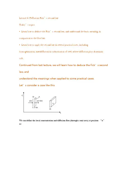
Lecture 4: Diffusion: Fick’s second lawToday’s topics•Learn how to deduce the Fick’s second law, and understand the basic meaning, in comparison to the first law.•Learn how to apply the second law in several practical cases, including homogenization, interdiffusion in carburization of steel, where diffusion plays dominant role.Continued from last lecture, we will learn how to deduce the Fick’s second law, andunderstand the meanings when applied to some practical cases.Let’s consider a case like thisWe can define the local concentration and diffusion flux (through a unit area) at position “x”as:So, Fick’s first law can be considered as a specific (simplified) format of the second law when applied to a steady state.Now, let’s consider two real practical cases, and see how to solve the Fick’s second law in these specific cases.Case 1. Homogenization: (non-uniform →uniform)Consider a composition profile as superimposed sinusoidal variation as shown below, where the solid line represents the initial concentration profile (at t=0), and the dashed line represents the profile after time τ.It is an exponential decay, the longer the wavelength (l), the longer the relaxation time (τ), then the slower decay. Short wavelength dies fast. That’s why shaking always helps speed up the dispersion, because it enables wide spreading (smaller l) of the stuff (like particles) youtry to disperseCase 2. Interdiffusion (the carburization of steel):doping of steel with carbonSituation a): Doping with fixed amount of dopantConsider a thin layer of B deposited onto A, through annealing at high temperature, we will be able to get the concentration profile at different times, from there then we can determine the diffusion coefficient, Das determined by this diffusion kinetics equation, the concentration profile of carbon as various times will be like thisThe above diffusion is one-direction (0 →+∞). But if we extends it to two-way, from -∞to +∞(like a droplet dissolved into a solution) with dopant at x=0, then we haveSituation b): Doping with a fixed surface concentration (e.g. carburization of steel)Carbon concentration profile shown at different times,Carbonization thickness is defined asThe solution of the Fick’s second law can be obtained as follows, the surface is in contact with an infinite long reservoir of fixed concentration of , choose a coordinate system u.Interdiffusion is popular between two semi-infinite specimens of different compositions c1, c2, when they are joined together and annealed, or mixed in case of two solutions (liquids). Many examples in practice fall into the case interdiffusion, including two semiconductor interface, metal-semiconductor interface, etc.。
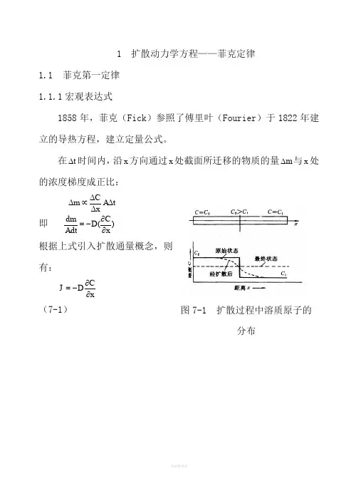
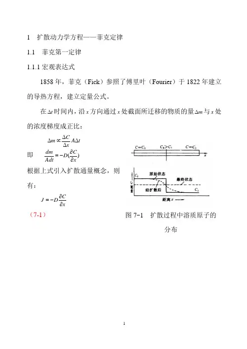
1 扩散动力学方程——菲克定律1.1 菲克第一定律 1.1.1宏观表达式1858年,菲克(Fick )参照了傅里叶(Fourier )于1822年建立的导热方程,建立定量公式。
在t ∆时间内,沿x 方向通过x 处截面所迁移的物质的量m ∆与x 处的浓度梯度成正比:t A xCm ∆∆∆∝∆ 即 )(xCD Adt dm ∂∂-=根据上式引入扩散通量概念,则有:xCDJ ∂∂-=(7-1)图7-1 扩散过程中溶质原子的分布式(7-1)即菲克第一定律。
式中J 称为扩散通量,常用单位是mol /()2s cm ⋅;xC∂∂浓度梯度; D 扩散系数,它表示单位浓度梯度下的通量,单位为2cm /s 或s m /2; 负号表示扩散方向与浓度梯度方向相反见图7-2。
1.1.2微观表达式微观模型:设任选的参考平面1、平面2上扩散原子面密度分别为n 1和n 2,若n 1=n 2,则无净扩散流。
假定原子在平衡位置的振动周期为τ,则一个原子单位时间内离开相对平衡位置跃迁次数的平均值,即跃迁频率Γ为τ1=Γ (7-2)由于每个坐标轴有正、负两个方向,所以向给定坐标轴正向跃迁的几率是Γ61。
设由平面l 向平面2的跳动原子通量为J 12,由平面2向平面1的跳动原图7-2 溶质原子流动的方向与浓度降低的方向相一致图7-3 一维扩散的微观模型子通量为J 21Γ=11261n J (7-3)Γ=22161n J (7-4) 注意到正、反两个方向,则通过平面1沿x 方向的扩散通量为 ()212112161n n J J J -Γ=-= (7-5) 而浓度可表示为 δδnn C =⋅⋅=11 (7-6) 式(7-6)中的1表示取代单位面积计算,δ表示沿扩散方向的跳动距离(见图7-3),则由式(7-5)、式(7-6)得 ()dxdCDdx dC C C C C J -=Γ-=-Γ-=-Γ=21221161)(6161δδδ (7-7) 式(7-7)即菲克第一定律的微观表达式,其中261δΓ=D (7-8) 式(7-8)反映了扩散系数与晶体结构微观参量之间的关系,是扩散系数的微观表达式。
包括两个内容:(1)早在1855年,菲克就提出了:在单位时间内通过垂直于扩散方向的单位截面积律是在第一定律的基础上推导出来的。
菲克第二定律指出,在非稳态扩散过程中,在距离x处,浓度随时间的变化率等于该处的扩散通量随距离变化率的负值,费克第一定律早在1855年,菲克就提出了:在单位时间内通过垂直于扩散方向的单位截面积的扩散物质流量(称为扩散通量Diffusion flux,用J表示)与该截面处的浓度梯度(Concentration gradient)成正比,也就是说,浓度梯度越大,扩散通量越大。
这就是菲克第一定律,它的数学表达式如下: (1)式(1)中, D称为扩散系数(m²/s),C为扩散物质(组元)的体积浓度(原子数/m³或kg/m³),dC/dx 为浓度梯度,―–‖号表示扩散方向为浓度梯度的反方向,即扩散组元由高浓度区向低浓度区扩散。
扩散通量J的单位是kg / m^2·s。
在三维情况下,有如下形式公式:其中,J为扩散通量,为一个三维向量场,D为扩散系数,为一个二阶张量,C为浓度,为一个数量场,▽为梯度算子。
扩散系数(Diffusion coefficient)D是描述扩散速度的重要物理量,它相当于浓度梯度为1时的扩散通量,D值越大则扩散越快。
对于固态金属中的扩散,D值都是很小的,例如,1000℃时碳在γ-Fe 中的扩散系数D仅为10m^2/s数量级。
费克定律里的稳态扩散和非稳态扩散费克第一定律只适应于J和C不随时间变化——稳态扩散(Steady-state diffusion)的场合(见下图)。
对于稳态扩散也可以描述为:在扩散过程中,各处的扩散组元的浓度C只随距离x变化,而不随时间t变化,每一时刻从前边扩散来多少原子,就向后边扩散走多少原子,没有盈亏,所以浓度不随时间变化。
实际上,大多数扩散过程都是在非稳态条件下进行的。
非稳态扩散(Nonsteady-state diffusion)的特点是:在扩散过程中,J随时间和距离变化。
1 扩散动力学方程——菲克定律1.1 菲克第一定律 1.1.1宏观表达式1858年,菲克(Fick )参照了傅里叶(Fourier )于1822年建立的导热方程,建立定量公式。
在t ∆时间内,沿x 方向通过x 处截面所迁移的物质的量m ∆与x 处的浓度梯度成正比:t A xCm ∆∆∆∝∆ 即 )(xCD Adt dm ∂∂-=根据上式引入扩散通量概念,则有:xCDJ ∂∂-=(7-1)图7-1 扩散过程中溶质原子的分布式(7-1)即菲克第一定律。
式中J 称为扩散通量,常用单位是mol /()2s cm ⋅;xC∂∂浓度梯度; D 扩散系数,它表示单位浓度梯度下的通量,单位为2cm /s 或s m /2; 负号表示扩散方向与浓度梯度方向相反见图7-2。
1.1.2微观表达式微观模型:设任选的参考平面1、平面2上扩散原子面密度分别为n 1和n 2,若n 1=n 2,则无净扩散流。
假定原子在平衡位置的振动周期为τ,则一个原子单位时间内离开相对平衡位置跃迁次数的平均值,即跃迁频率Γ为τ1=Γ (7-2)由于每个坐标轴有正、负两个方向,所以向给定坐标轴正向跃迁的几率是Γ61。
设由平面l 向平面2的跳动原子通量为J 12,由平面2向平面1的跳动原图7-2 溶质原子流动的方向与浓度降低的方向相一致图7-3 一维扩散的微观模型子通量为J 21Γ=11261n J (7-3)Γ=22161n J (7-4) 注意到正、反两个方向,则通过平面1沿x 方向的扩散通量为 ()212112161n n J J J -Γ=-= (7-5) 而浓度可表示为 δδnn C =⋅⋅=11 (7-6) 式(7-6)中的1表示取代单位面积计算,δ表示沿扩散方向的跳动距离(见图7-3),则由式(7-5)、式(7-6)得 ()dxdCDdx dC C C C C J -=Γ-=-Γ-=-Γ=21221161)(6161δδδ (7-7) 式(7-7)即菲克第一定律的微观表达式,其中261δΓ=D (7-8) 式(7-8)反映了扩散系数与晶体结构微观参量之间的关系,是扩散系数的微观表达式。


Fickle第一定律,稳态扩散,一定时间内浓度不随时间变化,扩散通量(单位时间通过垂直于扩散方向的单位截面积的扩散物质流量)与浓度梯度成正比。
J=-D(dc/dx)扩散通量方向与浓度梯度方向相反
J,扩散通量;D,扩散系数,D=0.5(dx)2f(f,离子平均跳动频率)
Fickle第二定律,非稳态扩散,浓度随时间变化而变化
∂c/∂t=-D∂2c/∂x2,下面给出两种简单但常见的解:
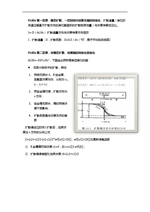
无限大物体中的扩散,假设
1.两根无限长A、B合金棒,
各截面浓度均匀,分别为c2、
c1,c2> c1;
2.两合金棒对焊,扩散方向为
x方向;
3.合金棒无限长,棒的两端浓
度不受影响;
4.扩散系数是与浓度无关的常
数
扩散偶经过时间t扩散后,溶质浓
度沿x方向的分布公式
C=(c2+c1)/2-(c2-c1)/2*erf[x/(2√Dt)],erf[x/(2√Dt)]为高斯误差函数
1)B金属棒初始浓度c1=0,则c=c2[1-erf(β)];
2)扩散偶焊接面处溶质浓度c0=(c2+c1)/2
半无限大物体中的扩散 c=c0[1-erf(β)]。
扩散方程扩散方程稳态扩散与非稳态扩散1.稳态扩散下的菲克第一定律(一定时间内,浓度不随时间变化dc/dt=0)单位时间内通过垂直于扩散方向的单位截面积的扩散物质流量(扩散通量)与该面积处的浓度梯度成正比即J=-D(dc/dx)其中D:扩散系数,cm2/s,J:扩散通量,g/cm2·s ,式中负号表明扩散通量的方向与浓度梯度方向相反。
可见,只要存在浓度梯度,就会引起原子的扩散。
x轴上两单位面积1和2,间距dx,面上原子浓度为C1、C2则平面1到平面2上原子数n1=C1dx ,平面2到平面1上原子数n2=C2dx若原子平均跳动频率f, dt时间内跳离平面1的原子数为n1f·dt跳离平面2的原子数为n2fdt,但沿一个方向只有1/2的几率,则单位时间内两者的差值即扩散原子净流量。
令,则上式2.扩散系数的测定:其中一种方法可通过碳在γ-Fe中的扩散来测定纯Fe的空心园筒,心部通渗碳气氛,外部为脱碳气氛,在一定温度下经过一定时间后,碳原子从内壁渗入,外壁渗出达到平衡,则为稳态扩散单位时单位面积中碳流量:A:圆筒总面积,r及L:园筒半径及长度,q:通过圆筒的碳量则:即:则:q可通过炉内脱碳气体的增碳求得,再通过剥层法测出不同r处的碳含量,作出C-lnr曲线可求得D。
第一定律可用来处理扩散中浓度不因时间变化的问3.菲克第二定律:解决溶质浓度随时间变化的情况,即dc/dt≠0两个相距dx垂直x轴的平面组成的微体积,J1、J2为进入、流出两平面间的扩散通量,扩散中浓度变化为,则单元体积中溶质积累速率为(Fick第一定律)(Fick第一定律),,,(即第二个面的扩散通量为第一个面注入的溶质与在这一段距离内溶质浓度变化引起的扩散通量之和)若D不随浓度变化,则故:4.Fick第二定律的解:很复杂,只给出两个较简单但常见问题的解a. 无限大物体中的扩散设:1)两根无限长A、B合?金棒,各截面浓度均匀,浓度C2>C1 2)两合金棒对焊,扩散方向为x方向3)合金棒无限长,棒的两端浓度不受扩散影响4)扩散系数D是与浓度无关的常数根据上述条件可写出初始条件及边界条件初始条件:t=0时, x>0则C=C1,x<0, C=C2边界条件:t≥0时, x=∞,C=C1, x=-∞, C=C2令,代入则,则菲克第二定律为即(1)令代入式(1)则有(2)若代入(2)左边化简有而积分有(3)令,式(3)为由高斯误差积分:应用初始条件t=0时x>0, c=c1,x<0, c=c2,从式(4)求得(5)则可求得(6)将(5)和(6)代入(4)有:,,,,,,,,,,,,上式即为扩散偶经过时间t扩散之后,溶质浓度沿x方向的分布公式,其中为高斯误差函数,可用表查出:根据不同条件,无限大物体中扩散有不同情况(1)B金属棒初始浓度,则(2)扩散偶焊接面处溶质浓度c0,根据x=0时,,则,若B棒初始浓度,则。
fick第一定律推导Fick's first law of diffusion states that the flux of a solute through a medium is directly proportional to the concentration gradient of the solute. Mathematically, it can be expressed as:J = -D * dC/dxwhere J is the flux of the solute (in units of mass per unit area per unit time), D is the diffusion coefficient or diffusivity of the solute (in units of area per unit time), C is the concentration of the solute, and x is the distance along which diffusion occurs.To derive this equation, let's consider a one-dimensional system where diffusion occurs along the x-axis. We assume that there are no other factors affecting the diffusion process, such as convection or reaction.First, consider a thin slice of the medium with a thickness dx. The flux of the solute across this slice can be defined as the rate at which the solute crosses a unit area of the slice, which can be written as J = -(dm/dt) / A, where dm is the mass of solute crossing the slice in a small time dt, and A is the area of the slice.Next, we can relate the mass crossing the slice to the concentration gradient by considering the change in concentration over a distance dx. This can be written as dC = (C2 - C1) / dx, where C1 and C2 are the concentrations of the solute at the boundaries of the slice. Assuming that the solute diffuses from higher concentration to lower concentration, we can write dm = -D * A * dC, where D isthe diffusion coefficient.Substituting these expressions into the flux equation, we get:J = -(dm/dt) / A= -(d/dt)(-D * A * dC) / A= D * dC/dtTo eliminate the time dependence and express the flux in terms of the spatial concentration gradient, we consider the chain rule and rewrite the equation as:J = D * (dC/dt) * (dt/dx)Since dx is a small distance and the solute is assumed to move with constant velocity, dt/dx can be approximated as v, where v is the velocity at which the solute diffuses.Thus, we get:J = D * v * dC/dxFinally, accounting for the direction of diffusion, we include a negative sign to indicate that diffusion occurs from higher to lower concentration, resulting in the final form of Fick's first law:J = -D * dC/dx。
fick扩散定律怎么拟合摘要:I.引言- 介绍Fick 扩散定律- 说明Fick 扩散定律拟合的意义和应用II.Fick 扩散定律的原理- 扩散的定义- Fick 第一定律- Fick 第二定律III.Fick 扩散定律的拟合方法- 概述拟合方法- 详细介绍常用拟合方法1.线性拟合2.非线性拟合3.插值拟合4.最小二乘法IV.拟合过程中的注意事项- 数据质量的重要性- 选择合适的拟合方法- 检验拟合效果V.结论- 总结Fick 扩散定律的拟合过程- 强调拟合结果的可靠性和实用性正文:Fick 扩散定律是描述物质扩散过程的基本定律,它在化学、物理、生物等多个领域都有广泛的应用。
对于科研工作者来说,如何准确地拟合Fick 扩散定律,从而更好地理解和研究相关现象,具有重要的意义。
本文将详细介绍Fick 扩散定律的拟合方法及注意事项。
首先,我们需要了解Fick 扩散定律的原理。
扩散是指物质由高浓度区域向低浓度区域的自发迁移过程。
Fick 扩散定律分为第一定律和第二定律。
Fick 第一定律指出,物质的扩散量与扩散系数成正比,与浓度梯度成反比;Fick 第二定律则说明,物质的扩散量与扩散系数和浓度梯度的乘积成正比。
在了解了Fick 扩散定律的原理之后,我们来探讨如何进行拟合。
拟合Fick 扩散定律的方法有很多,常用的有线性拟合、非线性拟合、插值拟合和最小二乘法等。
线性拟合适用于数据变化较为平缓的情况;非线性拟合可以更好地处理数据中的拐点和突变;插值拟合则是在已有数据点之间进行插值,以获得更连续的拟合曲线;最小二乘法则是通过最小化误差平方和来求解拟合方程,适用于各种类型的数据。
在拟合过程中,需要注意以下几点。
首先,数据质量是拟合的基础,要确保数据的准确性和完整性。
其次,选择合适的拟合方法,以适应数据的特点。
最后,检验拟合效果,通过对比实验数据和拟合曲线,评估拟合的准确性和实用性。
温 度表面碳浓度ρs/%试验回归值14.8173566150.8试验回归值2 4.5534427880.8回归平均值计算 4.6853997010.8试验回归值110.439278690.8试验回归值210.439278690.8回归平均值计算10.439278690.8试验回归值1#DIV/0!试验回归值2#DIV/0!回归平均值计算#DIV/0!试验回归值1#DIV/0!试验回归值2#DIV/0!回归平均值计算#DIV/0!试验回归值1#DIV/0!试验回归值2#DIV/0!回归平均值计算#DIV/0!温度/℃扩散常数Do(10-5m 2/s)扩散激活能Q(103J/mol)扩散系数D(10-12m 2/s)87021408.011148976927214016.12613347碳在γ-Fe扩散系数(10-12m 2/s)1、蓝色部分需要输入数值;2、白色部分为中间推导值;3、绿色部分为最终函数结果。
870Arrhenius方程:R为气体常数,其值为8.314J/(mol*K);Q代表每摩尔原子的激活能,T为绝对温度Gauss solution误差函数:FICK定律是按照扩散常熟不变进行计算的,而实际上随着渗碳的进行,奥氏体中碳的扩散常数是增距离表面X处界限碳浓度ρx/%芯部含碳量ρ0/%中间推导值Erf(β)β渗碳界限层深x/mm 0.350.180.7258064520.77320.720.350.180.7258064520.77320.70.350.180.7258064520.77320.70.350.180.7258064520.77320.790.350.180.7258064520.77320.790.350.180.7258064520.77320.9#DIV/0!#DIV/0!#DIV/0!#DIV/0!#DIV/0!#DIV/0!#DIV/0!#DIV/0!#DIV/0!进行,奥氏体中碳的扩散常数是增加的。
7.1 扩散定律(1)7.1.1 菲克第一定律(Fick’s First Law)扩散过程可以分类为稳态和非稳态。
在稳态扩散中,单位时间内通过垂直于给定方向的单位面积的净原子数(称为通量)不随时间变化,即任一点的浓度不随时间变化。
在非稳态扩散中,通量随时间而变化。
研究扩散时首先遇到的是扩散速率问题。
菲克(A. Fick)在1855年提出了菲克第一定律,将扩散通量和浓度梯度联系起来。
菲克第一定律指出,在稳态扩散(即)的条件下,单位时间内通过垂直于扩散方向的单位面积的扩散物质量(通称扩散通量)与该截面处的浓度梯度成正比。
为简便起见,仅考虑单向扩散问题。
设扩散沿x轴方向进行(图7-1),菲克第一定律的表达式为(7-1)式中:J为扩散通量(atoms/(m2·s)或kg/(m2·s));D为扩散系数(m2/s);为浓度梯度(atoms/(m3·m)或kg/(m3·m)) (图7-2为浓度梯度示意图);“-”号表示扩散方向为浓度梯度的反方向,即扩散由高浓度向低浓度区进行。
此方程又称为扩散第一方程。
当扩散在稳态条件下应用(7-1)式相当方便。
7.1.2 菲克第二定律(Fick’s Second Law)实际上,大多数重要的扩散是非稳态的,在扩散过程中扩散物质的浓度随时间而变化,即dc/dx≠0。
为了研究这种情况,根据扩散物质的质量平衡,在菲克第一定律的基础上推导出了菲克第二定律,用以分析非稳态扩散。
在一维情况下,菲克第二定律的表达式为(7-2)式中:为扩散物质的体积浓度(atoms/m3或kg/m3);为扩散时间(s);为扩散距离(m)。
(7-2)式给出c=f(t,x)函数关系。
式(7-2)又称为扩散第二方程。
由扩散过程的初始条件和边界条件可求出(7-2)式的通解。
利用通解可解决包括非稳态扩散的具体扩散问题。
7.1.3 扩散方程的求解1. 扩散第一方程扩散第一方程可直接用于描述稳定扩散过程。