最短路径文献翻译终极版
- 格式:doc
- 大小:1.30 MB
- 文档页数:19

本科毕业设计论文题目名称:最短路径算法的研究学院:计算机科学技术专业年级:计算机科学与技术(师范)级学生姓名:班级学号:2 班 13 号指导教师:二○一二年六月八日摘要本文目的在于研究关于最短路径的算法,为研究最短路径问题在一些出行问题、管理问题、工程问题及实际生活问题中的应用,为企业和个人提供方便的选择方法。
同时,也为其他的同学提供一些解题的思路与方法,为他们提供有利的资源。
最后应用蚁群算法来解决浙江旅行商问题。
通过应用最短路径算法中的蚁群算法来解决浙江旅行商问题,以各城市经纬度作为初始条件,通过 MATLAB 程序计算最短路径,并画出最短路线图。
关键词:最短路径算法;最短路径应用;蚁群算法;浙江旅行商精品毕业论文Abstract In this paper the purpose is to collect the shortest path algorithmabout common for the shortest path problem in some travel problemsmanagement engineering problems and practical application of life forenterprise and individual with convenient selection method. At the sametime the students for the mathematical modeling provide some ideas andmethods for problem solving provide favorable resources for the game.At last by use of ant colony algorithm to solve the zhejiang travelingsalesman problem. Through the application of the shortest path algorithm of ant colonyalgorithm to solve the zhejiang traveling salesman problem in the cityas the coordinates of initial conditions through the MATLAB calculationshortest paths and draw the shortest route map Key words:The shortest path algorithm The shortest path applicationant colony algorithm Zhejiang traveling salesma 精品毕业论文目录摘要 ........................................................................................................................................... IAbstract................................................................................................................................. ..........II第1章绪论...............................................................................................................................1 1.1 选题的意义及目的. (1)1.1.1 选题的意义 (1)1.1.2 选题的目的...........................................................................................................1 1.2 选题经过及国内外动态. (1)1.2.1 选题经过 (1)1.2.2选题的国内外动态...............................................................................................2第2章最短路径算法的介绍...................................................................................................3 2.1 Dijkstra 算法. (3)2.1.1 算法介绍及适用条件和范围 (3)2.1.2 算法描述和算法实现 (3)2.1.3 具体算法分析.......................................................................................................4 2.2A 算法 (8)2.2.1 算法介绍及适用条件和范围 (8)2.2.2 算法描述和算法实现 (9)2.2.3 具体算法分析.......................................................................................................9 2.3 Bellman-Ford 算法 (11)2.3.1 算法介绍及适用条件和范围 (11)2.3.2 算法描述和算法实现 (11)2.3.3 具体算法设计.....................................................................................................12 2.4 Topological Sort 算法 ..............................................................................................15 2.4.1算法介绍及适用条件和范围.............................................................................15 2.4.2算法描述和算法实现.........................................................................................16 2.4.3具体算法设计.....................................................................................................16 2.5 SSSP On DAG 算法 .. (20)2.5.1 算法介绍及适用条件和范围 (20)2.5.2 算法描述和算法实现.........................................................................................21 2.6 Floyd 算法 (21)2.6.1 算法介绍及适用条件和范围 (21)2.6.2 算法描述和算法实现 (21)2.6.3 算法具体分析.....................................................................................................22第3 章最短路径算法的比较 ................................................................................................26第 4 章最短路径算法的应用 (28)4.1 TSP问题的介绍 ............................................................................................................28 4.2 TSP 问题算法的介绍. (28)4.2.1 贪心算法 (28)4.2.2 模拟退火算法 (29)4.2.3 遗传序列算法 (29)精品毕业论文 4.2.4蚁群算法.............................................................................................................30 4.3算法应用 (31)4.3.1 解决浙江旅行商问题时算法描述 (31)4.3.2 蚁群算法的算法描述 (31)4.3.3 蚁群算法解决浙江旅行商问题.........................................................................34第5 章最短路径算法的展望 (36)绪论 (38)致谢 (39)参考文献 ............................................................................................................................... ........40 精品毕业论文第1章绪论1.1 选题的意义及目的1.1.1 选题的意义随着计算机科学的发展,人们生产生活经济利润的提高,最短路径问题逐渐成为计算机科学、运筹学、地理信息科学等学科的一个研究热点。
迪克斯特林算法的改进及在路线规划中的应用摘要:为了提高路网路线规划的效率,许多专家学者对此进行了一些研究。
Dijk stra算法是一个研究热点。
在两点之间寻找一个最佳路径时迪克斯特拉算法也有自己的缺点,但它仍具有无可替代的优势。
通过对经典Dijk stra算法优势和劣势的分析,我们可以发现,主要缺点可以概括为两点:存储结构和搜索区域。
因此,本文改进了这两点,即数据存储结构和限制算法搜索区域的改进。
通过分析实验结果获得其有效性。
关键词:迪克斯特拉算法;道路网络;路线规划;存储结构;受限搜索区域Ⅰ引言基于拓扑结构的道路网络,路线规划是为车辆运行期间到达目的地而进行的一种搜索最佳路径的过程以及车辆导航系统中最短路径问题的一种具体应用。
迪克斯特拉算法是在图中搜索最短路径最经典最成熟的算法,然而,该算法具有较高的时间复杂度以及要占有较大的存储空间。
为了克服迪克斯特拉算法的这些缺点,专家学者也相应做了大量的研究,他们的研究成果有各自的特点和优点,但相关算法的理论基础是迪克斯特拉算法,结合实际交通网络的分布特性,此论文改进了经典的迪克斯特拉算法以减少时间复杂度和存储空间,和减少算法的搜索规模,以此提高算法的运行效率。
Ⅱ存储结构A 存储结构的改进运用图片说明存储结构的改进原则,如图片1所示,采用邻接矩阵存储迪克斯特拉算法的数据,图片2显示各节点之间拓扑关系的邻接矩阵的结构,采用一个10×10的矩阵来存储点与点之间的拓扑关系,行与列同等数目。
矩阵[xi,xj]的值对应于节点i和j之间的权值,当源节点和末节点是同一个节点时,权值为0,两节点之间无直接路径时权值为∞。
此矩阵含有大量的0和∞,这也增加了无效路径的数目并占有了存储的大量空间。
因此从时间和空间的角度来看是不科0 2 ∞∞∞∞∞ 3 ∞∞ 4 3 2 0 4∞∞∞∞ 3 2 ∞∞ 4 0 3 ∞∞∞∞∞∞∞∞ 3 0 5 2 ∞∞ 3 ∞∞∞∞ 5 0 4 ∞∞∞∞∞∞∞ 2 4 0 3 ∞∞∞∞∞∞∞∞ 3 0 4 ∞ 13 3∞∞∞∞4 0 ∞∞∞ 2 ∞ 3 ∞∞∞∞ 0 5∞∞∞∞∞∞ 1 ∞ 5 0图片1,拓扑结构图片2,邻接矩阵关于上面提到存储模式,通过减少不必要的0和∞来压缩数据存储空间,用邻接表来存储数据。
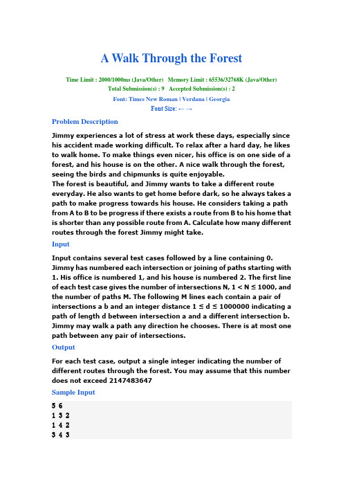
A Walk Through the ForestTime Limit : 2000/1000ms (Java/Other) Memory Limit : 65536/32768K (Java/Other)Total Submission(s) : 9 Accepted Submission(s) : 2Font: Times New Roman | Verdana | GeorgiaFont Size: ← →Problem DescriptionJimmy experiences a lot of stress at work these days, especially since his accident made working difficult. To relax after a hard day, he likes to walk home. To make things even nicer, his office is on one side of a forest, and his house is on the other. A nice walk through the forest, seeing the birds and chipmunks is quite enjoyable.The forest is beautiful, and Jimmy wants to take a different route everyday. He also wants to get home before dark, so he always takes a path to make progress towards his house. He considers taking a path from A to B to be progress if there exists a route from B to his home that is shorter than any possible route from A. Calculate how many different routes through the forest Jimmy might take.InputInput contains several test cases followed by a line containing 0. Jimmy has numbered each intersection or joining of paths starting with 1. His office is numbered 1, and his house is numbered 2. The first line of each test case gives the number of intersections N, 1 < N ≤ 1000, and the number of paths M. The following M lines each contain a pair of intersections a b and an integer distance 1 ≤ d ≤ 1000000 indicating a path of length d between intersection a and a different intersection b. Jimmy may walk a path any direction he chooses. There is at most one path between any pair of intersections.OutputFor each test case, output a single integer indicating the number of different routes through the forest. You may assume that this number does not exceed 2147483647Sample Input5 61 3 21 4 23 4 31 5 124 2 345 2 247 81 3 11 4 13 7 17 4 17 5 16 7 15 2 16 2 1Sample Output24对题意的理解:从点1 出发到点2;问满足条件的路径有多少条。

最短路径算法在空间移动对象网络数据库中的应用萧兰银,支明丁,李靖摘要一个在空间网络数据库查询的最重要(SNDB)支持基于位置的服务(LBS)是最短路径查询。
给定一个对象在一个网络中,例如一个位置的汽车在一个道路网络,和一组利益的对象,如酒店,加油站和汽车,最短路径查询返回的最短路径从感兴趣的对象的查询对象。
最短的研究路径查询有在线处理和预处理两种方式。
预处理假设兴趣对象的研究是静态的。
本文提出了一种最短路径算法的一组索引结构,支持移动对象的情况。
这算法可以动态问题转化为静态问题。
在本文中,我们重点对道路网络。
然而,我们的算法不使用任何特定的信息,因此可以适用于任何网络。
该算法的复杂度为O,和传统的Dijkstra的复杂度为O(+ K))。
关键词:移动对象;空间网络数据库;最短路径索引;最短路径第一章介绍随着无线通信的不断增长定位技术的发展,许多高效的查询移动对象和查询方法基于位置的服务(LBS)变得越来越重要。
此外,空间中的最短路径查询网络数据库是一种应用最广泛的服务。
Dijkstra的主动性工作之后,许多研究采用多种方法和算法解决问题最短路径查询已进行。
在最短路径研究的两fi领域算法:在线计算和预计算。
在线计算已经得到解决,例如,在最好绑定在预先计算中出现在,第二最好的算法在最短路径研究。
以前的工作的精确算法预处理包括那些使用几何信息,层次分解,概念达到,和A*搜索结合地标分布—。
该方法是计算最佳根据实时时间间隔中的路径。
这方法可以解决网络的动态变化和移动对象,但它需要太多的资源在每一个计算。
因此,计算时间太长,当网络规模较大,它不能提供实时的结果。
文献31讨论了如何重新计算路径快如果网络结构—真正的改变时,最短路径的计算。
在本文中,我们提出的算法在交通—性网络,但我们的算法不使用任何信息—网络环境相关。
因此,该算法可以在其他网络环境中使用。
我们现在讨论一些工作相关的预计算下面。
在这些算法中有两个复合部分:预处理算法计算的辅助数据,并查询算法和辅助计算最短路径—实验数据。
专业译文最短路的算法:以实际道路网络作为评估班级:2010122 姓名:张菲菲学号:20102322文章摘自:F. BENJAMIN ZHAN,CHARLES E. NOON.Department of Geography and Planning, Management Science Program, The University of Tennessee, Knoxville, Tennessee 37996摘要:寻找最短路径网络的经典问题多年来一直是大家的研究目标。
这些研究成果已经导致了一些不同的算法和大量的实证研究结果与性能。
但是,之前的研究并没有在选择计算实际网络道路的最短路径问题方面提供一个明确的方向。
大多数最短路径算法的计算测试是基于没有实际网络道路特征的随机生成的网络。
在本文中,我们提供了一个利用各种各样现实道路网络的最短路径算法的客观评价。
在评估的基础上,一套为计算实际道路网络而推荐的最短路径算法是正确的。
这种评价应该是对研究人员和从业人员在运筹学,管理科学,交通运输,地理信息系统方面特别有用。
关键词:实际网络道路;随机生成的网络;Bellman–Ford算法;Dijkstra算法1.介绍最短路径的计算在很多网络和交通运输分析中都是一个重要的任务。
在发展上面,计算测试和最短路径算法的有效实现一直在相关科学方面保持着重要的研究课题,比如运筹学,管理科学,地理,交通运输和计算机科学。
(参见Dijkstra 算法,1959;表盘等,1979;Glover- Klingman算法和Philips,1985;Ahuja,1990;Goldberg和Radzik,1993)。
这些研究成果已经衍生出许多最短路径的算法,此外,对于算法的计算性能也有大量的实证研究。
(参见比如,Glover- Klingman 算法等,1985;Gallo和Pallottino,1988;Mondou ,Crainic,Nguyen,1991;Cherkassky,Goldberg,Radzik,1993)。
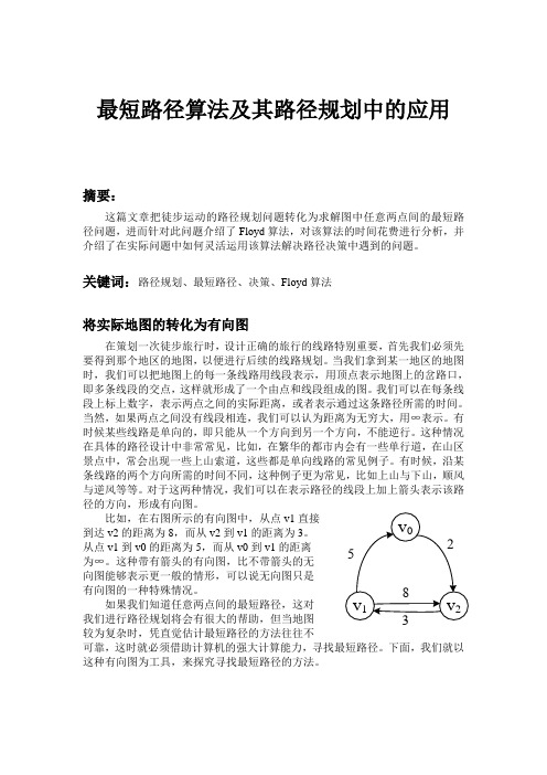
最短路径算法及其路径规划中的应用摘要:这篇文章把徒步运动的路径规划问题转化为求解图中任意两点间的最短路径问题,进而针对此问题介绍了Floyd算法,对该算法的时间花费进行分析,并介绍了在实际问题中如何灵活运用该算法解决路径决策中遇到的问题。
关键词:路径规划、最短路径、决策、Floyd算法将实际地图的转化为有向图在策划一次徒步旅行时,设计正确的旅行的线路特别重要,首先我们必须先要得到那个地区的地图,以便进行后续的线路规划。
当我们拿到某一地区的地图时,我们可以把地图上的每一条线路用线段表示,用顶点表示地图上的岔路口,即多条线段的交点,这样就形成了一个由点和线段组成的图。
我们可以在每条线段上标上数字,表示两点之间的实际距离,或者表示通过这条路径所需的时间。
当然,如果两点之间没有线段相连,我们可以认为距离为无穷大,用∞表示。
有时候某些线路是单向的,即只能从一个方向到另一个方向,不能逆行。
这种情况在具体的路径设计中非常常见,比如,在繁华的都市内会有一些单行道,在山区景点中,常会出现一些上山索道,这些都是单向线路的常见例子。
有时候,沿某条线路的两个方向所需的时间不同,这种例子更为常见,比如上山与下山,顺风与逆风等等。
对于这两种情况,我们可以在表示路径的线段上加上箭头表示该路径的方向,形成有向图。
到达v2的距离为8,而从v2到v1的距离为3。
从点v1到v0的距离为5,而从v0到v1的距离为∞。
这种带有箭头的有向图,比不带箭头的无向图能够表示更一般的情形,可以说无向图只是有向图的一种特殊情况。
如果我们知道任意两点间的最短路径,这对我们进行路径规划将会有很大的帮助,但当地图较为复杂时,凭直觉估计最短路径的方法往往不可靠,这时就必须借助计算机的强大计算能力,寻找最短路径。
下面,我们就以这种有向图为工具,来探究寻找最短路径的方法。
Floyd算法假设在一个景区中有n个景点,作为一个旅行团的领队,必需要知道这n 个景点中任意两个景点之间的最短路径,这时,我们可以使用Floyd算法。
图解迪杰斯特拉(Dijkstra)最短路径算法目录前言一、最短路径的概念及应用二、Dijkstra迪杰斯特拉1.什么是Dijkstra2.逻辑实现总结前言无论是什么程序都要和数据打交道,一个好的程序员会选择更优的数据结构来更好的解决问题,因此数据结构的重要性不言而喻。
数据结构的学习本质上是让我们能见到很多前辈在解决一些要求时间和空间的难点问题上设计出的一系列解决方法,我们可以在今后借鉴这些方法,也可以根据这些方法在遇到具体的新问题时提出自己的解决方法。
(所以各种定义等字眼就不用过度深究啦,每个人的表达方式不一样而已),在此以下的所有代码都是仅供参考,并不是唯一的答案,只要逻辑上能行的通,写出来的代码能达到相同的结果,并且在复杂度上差不多,就行了。
一、最短路径的概念及应用在介绍最短路径之前我们首先要明白两个概念:什么是源点,什么是终点?在一条路径中,起始的第一个节点叫做源点;终点:在一条路径中,最后一个的节点叫做终点;注意!源点和终点都只是相对于一条路径而言,每一条路径都会有相同或者不相同的源点和终点。
而最短路径这个词不用过多解释,就是其字面意思:在图中,对于非带权无向图而言,从源点到终点边最少的路径(也就是BFS广度优先的方法);而对于带权图而言,从源点到终点权值之和最少的路径叫最短路径;最短路径应用:道路规划;我们最关心的就是如何用代码去实现寻找最短路径,通过实现最短路径有两种算法:Dijkstra迪杰斯特拉算法和Floyd弗洛伊德算法,接下来我会详细讲解Dijkstra迪杰斯特拉算法;二、Dijkstra迪杰斯特拉1.什么是DijkstraDijkstra迪杰斯特拉是一种处理单源点的最短路径算法,就是说求从某一个节点到其他所有节点的最短路径就是Dijkstra;2.逻辑实现在Dijkstra中,我们需要引入一个辅助变量D(遇到解决不了的问题就加变量[_doge]),这个D我们把它设置为数组,数组里每一个数据表示当前所找到的从源点V开始到每一个节点Vi的最短路径长度,如果V到Vi有弧,那么就是每一个数据存储的就是弧的权值之和,否则就是无穷大;我们还需要两个数组P和Final,它们分别表示:源点到Vi的走过的路径向量,和当前已经求得的从源点到Vi的最短路径(也就是作为一个标记表示该节点已经加入到最短路径中了);那么对于如下这个带权无向图而言,我们应该如何去找到从V0到V8的最短路径呢;在上文中我们已经描述过了,在从V0到V8的这一条最短路径中,V0自然是源点,而V8自然是终点;于是我根据上文的描述具现化出如下的表格;在辅助向量D中,与源点V0有边的就填入边的权值,没边就是无穷大;构建了D、P和Final,那么我们要开始遍历V0,找V0的所有边中权值最短的的边,把它在D、P、Final中更新;具体是什么意识呢?在上述带权无向图中,我们可以得到与源点有关的边有(V0,V1)和(V0,V2),它们的权值分别是1和5,那么我们要找到的权值最短的的边,就是权值为1 的(V0,V1),所以把Final[1]置1,表示这个边已经加入到最短路径之中了;而原本从V0到V2的距离是5,现在找到了一条更短的从V0 -> V1 -> V2距离为4,所以D[2]更新为4,P[2]更新为1,表示源点到V2经过了V1的中转;继续遍历,找到从V0出发,路径最短并且final的值为0的节点。
本科毕业论文(设计) 论文题目:交通咨询系统的最短路径算法与实现****:**学号: **********专业:信息管理与信息系统班级:信管0201****:***完成日期:2015年 5月 5日目录序言 (1)一、绪论 (2)(一)课题的背景和意义 (2)(二)研究现状 (2)1.最短路径算法研究现状 (2)2.最短路径算法分类 (3)3.算法时间复杂度 (3)(三)研究内容 (4)(四)论文结构 (4)二、最短路径算法相关原理 (4)(一)D IJKSTRA算法 (4)1.算法思想分析 (5)2.实现思路 (5)3.计算步骤 (5)(二)F LOYD算法 (7)1.算法思想原理: (8)2.算法描述: (8)3.Floyd算法过程矩阵的计算----十字交叉法 (8)三、开发工具与环境 (10)(一)J AVA技术 (10)1. Java简介 (10)2.Java的处理流程 (11)四、交通咨询系统的实现 (11)(一)系统分析 (11)1.系统的设计内容: (11)2.系统的设计思想 (12)3.系统设计流程 (12)(二)系统功能结构 (12)1. 系统构架设计 (12)2.系统详细设计 (14)3. 测试数据及分析 (26)五、设计总结 (28)致谢 (29)参考文献 (29)交通咨询系统的最短路径算法与实现内容摘要目前在交通咨询领域,最短路径算法的研究和应用越来越多,其中最短路径算法的效率问题是普遍关注并且在实际应用中迫切需要解决的问题。
随着现代生活节奏的加快,以及城市汽车数量的不断增加,交通网络也越来越发达,在交通工具和交通方式不断更新的今天,人们在旅游、出差或者其他出行时,不仅会关心费用问题,而且对里程和所需要的时间等问题也特别感兴趣。
为了能够更方便人们的出行,我们就应该以最短路径问题建立一个交通咨询系统。
这样的一个交通系统可以回答人们提出的有关交通的所有问题,比如任意一个城市到其他城市的最短路径,或者任意两个城市之间的最短路径问题。
目录目录 (1)摘要 (3)Abstract (4)第一章绪论 (5)1.1课题背景 (5)1.2目的意义 (5)1.3国内外现状 (5)1.4重点工作 (6)第二章最短路径问题的基础知识 (7)2.1 图的基本概念 (7)2.2图的遍历 (8)2.2.1深度优先搜索 (8)2.2.2广度优先搜索 (9)第三章最短路径算法 (10)3.1 Dijkstra算法 (10)3.1.1 算法原理 (10)3.1.2 算法描述 (10)3.1.3算法步骤 (11)3.1.4 Dijkstra算法的应用举例 (11)3.1.5 Dijkstra算法的不足 (14)3.1.6 改进Dijkstra 算法的基本思想及实现 (14)3.2 bellman-ford算法 (14)3.2.1算法原理 (14)3.2.2算法描述 (15)3.2.3 bellman-ford算法的优缺点 (15)3.2.4 bellman-ford算法的优化 (15)3.3 Floyd算法 (16)3.3.1 算法原理 (16)3.3.2算法描述 (16)3.3.3 Floyd算法的优缺点 (17)第四章设计实现经典Dijkstra算法 (18)4.1程序运行环境 (18)4.2开发语言简介 (18)4.3 可行性分析 (20)4.4需求分析 (20)4.5 软件结构 (21)4.6 模块详细设计与实现 (21)4.6.1 程序流程图 (22)4.6.2 各模块设计 (22)4.7系统特色 (25)4.8 系统需要改进的地方 (25)第五章结论 (26)5.1 最短路径算法 (26)5.2 心得与收获 (26)致谢 (27)参考文献 (28)摘要随着社会的进步,科技的飞速发展,人们的办事效率也得到了极大的提高,在当今的社会里,花费最小的代价收获最大的效益,成为了当今社会里各行各业一直信奉的理念,这种理念最直接地体现在求最短路径的问题上,在生活中最常见的有通信问题、公交网络问题、旅游线路设计与优化中的运筹学问题等。
单位代码01学号*********分类号O24密级文献翻译最短通路问题院(系)名称信息工程学院专业名称信息与计算科学学生姓名许秀成指导教师孙贵玲2013年 3 月10日8. 6 最短通路问题8.6.1引言许多问题可以用边上赋权的图来建模。
考虑一下航线系统如何建模。
如果用顶点表示城市,用边表示航线。
给边赋上城市之间的距离,就可以为涉及距离的问题建模;给边赋上飞行时间,就可以为涉及飞行时间的问题建模;给边赋上票价,就可以为涉及票价的问题建模。
图8—61显示了给一个图的边赋权的三种不同方式,分别表示距离,飞行时间和票价。
波士顿波士顿 密图 8-61 为航线系统建模的带权图给每条边赋上一个数的图称为带权图。
带权图用来为计算机网络建模。
通信成本(比如租用电话线的月租费)、计算机在这些线路上的响应时间或是计算机之间的距离等都可以用带权图来研究。
图8—62显示一些带权图,它们表示给计算机的图的边赋权的三种方式,分别对应成本、响应时间和距离。
与带权图有关的几种类型的问题出现得很多。
确定网络里两个顶点之间长度最短的通路就是一个这样的问题。
说的更具体些,设带权图里一条通路的长度是这条通路上各边的权的总和。
(读者应当注意,对术语长度的这种用法,与表示不带权的图的通路里边数的长度的用法,这两者是不同的。
)问题是:什么是最短通路,即什么是在两个给定顶点之间长度最短的通路?例如,在图8—61所示带权图表示的航线系统里,在波士顿与洛杉矶之间以空中距离计算的最短通路是什么?在波士顿与洛杉矶之间什么样的航班组合的总飞行时间(即在空中的总时间,不包括航班之间的时间)最短?在这两个城市之间的最低费用是多少?波士顿距离达拉斯图 8-62 为计算机网络建模的带权图在图8—62所示的计算机网络里,连接旧金山的计算机与纽约的计算机所需要的最便宜的一组电话线是什么?哪一组电话线给出旧金山与纽约之间的通信的最短响应时间?哪一组电话线有最短的总距离?与带权图有关的另外的一个重要问题是:求访问完全图每个顶点恰好一次的、总长度最短的回路。
这就是著名的旅行商问题,它求一位推销商应当以什么样的顺序来访问其路程上的每个城市恰好一次,使得他旅行的总距离最短。
本节后面将讨论旅行商问题。
8.6.2 最短通路算法求带权图里两个顶点之间的最短通路有几个不同的算法。
下面将给出荷兰数学家E ·迪克斯特拉在1959年所发现的一个解决无向带权图中最短通路问题的算法,其中所有的权都是正数。
可以很容易地将它修改后来解决有向图里的最短通路问题。
响应时间达拉斯秒月租费达拉斯在给出这个算法的形式化表示之前将给出一个启发性的例子。
例 1 在图8—63所示的带权图里,a 和z 之间的最短通路的长度是多少?图 8—63解 虽然通过观察就容易求出最短通路,但是需要想出一些有助于理解迪克施特拉算法的办法。
要解决的问题就是:求从a 到各个相继的顶点的最短通路,直到到达z 为止。
从a 开始、(直到到达终点为止)不包括除a 以外的顶点的唯一通路是a ,b 和a ,d 。
因为a ,b 和a ,d 的长度分别是4和2,所以d 是与a 最近的顶点。
可以通过查看(直到到达终点为止)只经过a 和d 的所有通路,来求出下一个最靠近a 的顶点。
到b 的最短通路仍然是a ,b ,长度为4,而到e 的最短通路是a ,e d ,,长度为5。
所以,下一个与a 最靠近的顶点是b 。
为了找出第三个与a 最近的顶点,只需要检查(直到到达终点为止)只经过了d a ,和b 的那些通路。
存在长度为7到c 的通路,即c b a ,,,以及长度为6到z 的通路,即z ed a ,,,。
所以,z 是下一个与a 最靠近的顶点,而且到z 的最短通路的长度为6。
例 1 说明了在迪克斯特拉算法里使用的一般原理。
注意通过检查就可能求出从a 到z 最短通路。
不过,无论对人还是对计算机来说,检查边数很多的图都是不切实际的。
现在将考虑一般问题:在无向联通简单带权图里,求出a 与z 之间的最短通路的长度。
迪克斯特拉算法如下进行:求出从a 到第一个顶点的最短通路的长度,从a 到第二个顶点最短通路的长度,以此类推,直到求出a 到z 的最短通路长度为止。
这个算法依赖于一系列的迭代。
通过在每次跌代里添加一个顶点来构造出特殊顶点的集合。
在每次跌代里完成一个标记过程。
在这个标记过程,只包括特殊顶点的从a 到w 的最短通路的长度来标记w 。
添加到特殊顶点集里的顶点是尚在集合之外的那些顶点az中带有最小标记的顶点。
现在给出迪克斯特拉算法的细节。
它首先用0标记a 而用∞标记其余的顶点。
用记号0)(0=a L 和∞=)(0v L 表示在没有发生任何迭代之前的这些标记(下标0表示“第0次”迭代)。
这些标记是从a 到这些顶点的最短通路的长度,其中这些通路只包含顶点a 。
(因为不存在a 到其他顶点的这种通路,所以∞是a 与这样的顶点之间的最短通路的长度。
)迪克斯特拉算法是通过形成特殊顶点的集合来进行的。
设k s 表示在标记过程k 次迭代之后的特殊顶点集。
首先φ=0S 。
集合k s 是通过过程把不属于1-k s 的带最小标记的顶点u 添加到1-k s 里形成的,一旦把u 添加到k s 里,就更新所有不属于k s 的顶点的标记,使得顶点v 在第个阶段的标记k L ()v 是只包含k s 里顶点(即已有的特殊点再加上u )的、从a 到v 的最短通路的长度。
设v 是不属于k s 的一个顶点。
为了更新v 的标记,注意k L ()v 是只包含k s 里k 顶点的从a 到v 的最短通路,要么是只包含1-k s 里顶点(即不包括u 在内的特殊顶点)的从a 到v 的最短通路,要么1-k 阶段加上边(v u ,)的从a 到u 的最短通路。
换句话说,(){()()()}v u w u a L v a L v a L k k ,,,,m in ,11+=--这个过程这样迭代:相继添加顶点到特殊顶点集里,直到添加z 为止。
当把z 添加到特殊顶点集里时,它的标记就是从a 到z 的最短通路的长度。
在算法1里给出迪克斯特拉算法。
随后将证明这个算法的正确性。
算法1 迪克施特拉算法Procedure Dijkkstra(G :所有权都为正数的带权连通简单图){G 带有顶点z v v a ==,...1,0和权)(,j i v v w ,其中若},{j i v v 不是G 里的边,则)(,j i v v w =∞} For i:=1 to n)(i v L :=∞)(a L :=0 S :=φ{ 现在初始化标记,使得a 的标记为0而所有其余标记为∞,S 是空集合 } While z ∉S Beginu :=不属于S 的)(u L 最小的一个顶点S :=S }{uFor 所有不属于S 的顶点vIf )(u L ),(v u w +)(v L < then ),()(:)(v u w u L v L +={这样就给S 里添加带最小标记的顶点,而且更新不在S 里的顶点的标记} end =)({z L 从a 到z 的最短通路的长度}下面的例子说明迪克施特拉算法是如何工作的。
随后我们将证明这个算法总是产生带权图里两个顶点之间最短通路的长度。
例 2 用迪克施特拉算法求图8—64a 所示的带权图里顶点a 与z 之间最短通路的长度。
解 图8—64里显示了迪克斯特拉算法求a 与z 之间最短通路所用的步骤。
在算法的每次迭代里,用圆圈圈起集合k S 里的顶点。
对每次迭代都标明了只包含k S 里顶点的从a 到每个顶点的最短通路。
当圆圈圈到z 时,算法终止。
找到从a 到z 的最短通路是e d b c a ,,,,,长度为13。
下一步,用归纳论证来证明迪克斯特拉算法产生无向连通带权图里两个顶点a 与z 之间最短通路的长度。
用下列断言作为归纳假设:在第k 次迭代里 )(i S 里的顶点v )0(≠v 的标记是从a 到这个顶点的最短通路的长度。
)(ii 不在S 里的顶点的标记是(这个顶点自身除外)只包含S 里顶点的最短通路的长度。
当0=k 时,在没有执行任何迭代之前,}{a S =,所以从a 到除a 外的顶点的最短通路长度是∞。
设v 是第1+k 次迭代里添加到S 里的顶点,使得v 是在第k 次迭代结束时带最小标记的不在S 里的顶点不唯一的情形里,可以采用带最小标记的任意顶点。
根据归纳假设,可以看出在第1+k 次迭代之前,S 里的顶点都用从a 出发的最短通路的长度来标记。
图8-64 用迪克斯特拉算法求从a 到z 的最短距离另外,必须用从a 到v 的最短通路的长度来标记v 。
假如情况不是这样,那么在第k 次迭代结束时,就可能存在包含不在S 里的顶点的、长度小于)(v L k 的通路(因为)(v L k 是在第k 次迭代之后、只包含S 里顶点的、从a 到v 的最短通路的长度)。
设u 是在这样的通路里不属于S 的第一个顶点。
则存在一条只包含S 里顶点的、从a 到u 的长度小于)(v L k 的通路。
这与对v 的选择相矛盾。
因此,在第1+k 次迭代时)(i 成立。
设u 是在第1+k 次迭代之后不属于S 的一个顶点。
只包含S 里顶点的从a 到u 的最短通路要么包含v 、要么不包含v 。
若它不包含v ,则根据归纳假设,它的长度是)(u L k 。
若它确实包含v ,则它必然是这样组成的:一条只包含S 里除v 之外的顶点的、从a 到v 具有最短可能长度的通路,后面接着从v 到u 的边。
这种情形里它的长度是),()(u v w v L k +。
这样就证明了)(ii 为真,因为)},(min{)()(),(1u v w L L u L v k u k k +=+。
已经证明了定理1.定理1 迪克斯特拉算法求出连通简单无向带权图里两个顶点之间最短通路的长度。
现在可以估计迪克斯特拉算法的计算复杂性(就加法和比较而言)。
这个算法使用的迭代次数不超过n -1次,因为在每次迭代里添加一个顶点到特殊顶点集里。
若可以估计每次迭代所使用的运算次数,则大功告成。
可以用不超过n -1次比较来找出不在k S 里的带最小标记的顶点。
于是我们使用一次加法和一次比较来更新不在k S 中的每一个顶点的标记,所以在每次迭代里的运算不超过)1(2-n 次,因为在每次迭代里要更新的标记不超过n -1个。
因为迭代次数不超过n -1次,每次迭代的运算次数不超过)1(2-n ,所以有下面的定理。
定理 2 迪克斯特拉算法使用)(2n O 次运算(加法和比较)来求出连通简单无向带权图里两个顶点之间最短通路的长度。
来源于:罗森(美).离散数学及其应用.北京:机械工业出版社,2003.8(6):491-496.附:英文原文8.6 Shortest-Path Problems8.6.1 IntroductionMany problems can be modeled using graphs with weights assigned to their edges. As an illustration, consider how an airline system can be modeled. We set up the basic graph model by representing cities by vertices and flights by edges. Problems involving flight time can be modeled by assigning flight times to edges. Problems involving fares can be modeled by assigning fares to the edges. Figure 1 displays three different assignments of weights to the edges of a graph representing distances, flight times, and fares, respectively.Graphs that have a number assigned to each are called weighted graphs. Weighted graphs are used to model computer networks. Communications costs (such as the monthly cost of leasing a telephone line),the response times of the computers over these lines, or the distance between computer, can all be studied using weighted graphs, Figure 2 display weighted graphs that represent three ways to assign weights to the edges of a computer network, corresponding to distance, response time, and cost.Several types of problems involving weighted graphs arise frequently. Determining a path of least length between two vertices in a network is one such problem. To be more specific, let the length of a path in a weighted graph be the sum of the weights of the edges of this path.(The reader should note that this use of the term length is different from the use of length to denote the number of edges in a path in a graph without weights.)BostonThe question is: What is a shortest path, that is, a path of least length, between two given vertices? For instance, in the airline system represented by the weighted graph shown in Figure 1, what is a shortest path in air distance between Boston and Los Angles? What combinations of flights has the smallest total flight time (that is, total time in the air, not including time between flights) between Boston and Los Angels? What is the cheapest fare between these two cities? In the computer network shown in 2, what is a least expensive set of telephone lines gives a fastest response time for communications between San Francisco and New York? Which set of lines has a shortest overall distance?There are several different algorithms that find a shortest path between two vertices in a weighted graph. We will present an algorithm discovered by the Dutch mathematician Edger Dijkstra in 1959. The version we will describe solves this problem in undirected weighted graphs where all the weights are positive. It is easy to adapt it to solve shortest-path problems in directed graphs.BostonFIGURE 8-61 Weighted Graphs Modeling an Airline SystemAnother important problems involving weighted graphs asks for a lot of shortest totallength that visits every vertex of a complete graph exactly once. This is the famous traveling salesman problem,which asks for an order in which a salesman should visit each of the citieson his route exactly once so that he travels the minimum total distance. We will discuss the on traveling salesman problem later in this section.DISTANCEDallasRESPONSE TIMEDallasLEASE RATES(PER MONTH)DallasFIGURE 2 Weighted Graphs Modeling a Computer Network8.6.2 A Shortest-Path AlgorithmThere are several different algorithms that find a shortest path between two vertices in a weighted graph. We will present an algorithm discovered by the Dutch mathematician Edger Dijkstra in 1959. The version we will describe solves this problem in undirected weighted graphs where all the weights are positive. It is easy to adapt it to solve shortest-path problems in directed graphs.Before giving a formal presentation of the algorithm, we will give a motivating example. EXAMPLE 1What is the length of a shortest path between a and z in the weighted graph shown in Figure 3?FIGHER 8-63Solution: Although a shortest path is easily found by inspection , we will develop some ideas useful in understanding Dijkstra’s algorithm. We will solve this problem by finding the length of a shortest path from a to successive vertices, until z is reached.The only paths starting at a that contain no vertex other than a (until the terminal vertex is reached) are b a , and d a ,. Because the lengths of b a , and d a , are 4 and 2, respectively, it follows that d is the closest vertex to a .We can find the next closest vertex by looking at all paths that go through only a andd (until the terminal vertex is reached). The shortest such path to b is still b a ,, with length4,and the shortest such path to e is e d a ,,, with length 5.Consequently, the next closest vertex to a is b .To find the third closest vertex to a , we need to examine only paths that go through onlyd a , and b (until the terminal vertex is reached). There is a path of length 7 to c namelyc b a ,, and a path of length 6 to z , namely,ze d a ,,,. Consequently, z is the next closestvertex to a , and the length of a shortest path to z is 6.Example 1 illustrates the general principles used in Dijkstra’s algorithm. Note that ashortest path from a to z could have been found by inspection. However, inspection is impractical for both humans and computers for graphs with large numbers of edges.We will now consider the general problem of finding the length of a shortest path between a and z in an undirected connected simple weighed graph. Dijkstra’s algorithm proceeds by finding the length of a shortest path from a to a first vertex, the length ofaa zshortest path from a to a second vertex, and so on, until the length of a shortest from a toz is found.The algorithm relies on a series of iterations. A distinguished set of vertices is constructed by adding one vertex. A labeling procedure is carried out at earth iteration. In this labeling procedure, a vertex w is labeled with the length of a shortest path from a to w that contains only vertics already in the distinguished set. The vertex added to the distinguished set is one with a minimal label among those vertices not already in the set. We now give the details of Dijkstra’s algorithm. It begins by labeling a with 0 and the other vertices with ∞.We used the notation =)(0a L 0 and =)(0v L ∞ for these labels before any iterations have taken place (the subscript 0 stands for th e “0th” iteration). These labels are the lengths of shortest paths from a to the vertices, where the paths contain only the vertexa .(Because no path from a to a vertex different from a exists,∞ is the length of a shortest path between a and this vertex.)Dijkstra’s algorithm proceeds by forming a dist inguished set of vertices. Let k S denote this set after k iterations of the labeling procedure. We begin with =0S φ. The set k S is formed from 1-k S by adding a vertex u not in 1-k S with the smallest label. Once u is added to k S , we update the labels of all vertices not in k S , so that )(v L k ,the label of the vertex v at the kth stage, is the length of a shortest path from a to v that contains vertices only in k S (that is, vertices that were already in the distinguished set together withu ).Let v be a vertex not in k S . To update the label of v , note that )(v L k is the length of a shortest path from a to v containing only vertices in k S . The updating can be carried out efficiently when this observation is used: A shortest path from a to v containing only elements of k S is either a shortest path from a to v that contains only elements of1-k S (that is, the distinguished vertices not including u ), or it is a shortest path from a to uat the )1(-k st stage with the edge ),(v u added. In other words,(){()()()}v u w u a L v a L v a L k k ,,,,m in ,11+=--This procedure is iterated by successively, adding vertices to the distinguished set until z is added. When z is added to the distinguished set, its label is the length of a shortest path from a to z .Dijkstra’s algorithm is given in Algorithm 1. Later we will a proof that this algorithm is correct.ALGORITHM 1 Dijkstra’s Algorithm.Procedure Dijkkstra(G :weighted connected simple graph, with all weights positive)) {G has vertices z v v a ==,...1,0 and weighted )(,j i v v w ,where },{j i v v =∞ if )(,j i v v w is not an edge in G } For i:=1 to n)(i v L :=∞)(a L :=0 S :=φ{ the label are now initialized so that the label of a is 0 and all other labels are ∞,and S is the empty set } While z ∉S Beginu :=a vertex not in S with )(u L minimalS :=S }{uFor all vertices v not in SIf )(u L ),(v u w +)(v L < then ),()(:)(v u w u L v L +={this adds a vertex to S with minimal label and update the labels a vertices not in S }FIGURE 4 Using Dijkstra’s Algorithm to Find a Shortest Path from a to z illustrates how Dijkstra’s algorithm works. Afterwards, we will show that this algorithm always produces the length of a shortest path between two vertices in a weighted graph. EXAMPLE 2Use Dijkstra’s algorithm to find the length of a shortest path between the vertices a and z in the weighted graph displayed in Figure 4(a).Solution: The steps used by Dijkstra’s algorithm to find a shortest path between a and z are shown in Figure 4.Ateach iteration of the algorithm the vertices of the setS are circled.kA shortest path from a to each vertex containing only vertices inS is indicated for eachkiteration. The algorithm terminations when z is circled. We find that a shortest path from a to z is za,,,,,with length 13.cedbRemark: In performing Dijkstra’s algorithm it is sometimes more convenient to keep track of labels of vertices in each step using a table instead of rewarding the graph for each step.Next, we use an inductive arg ument to show that Dijkstra’s algorithm produces the length of a shortest path between two vertices a and z in an undirected connected weightedgraph. Take as the induction hypothesis the following assertion: At the k th teration. )(i the label of every vertex v in S is the length of a shortest path from a to this vertex ,and)(ii the label of every vertex note in S is the length of a shortest path from a to this vertex that contain only(besides the vertex itself) vertices in S .When 0=k , before any iterations are carried out,=S φ, so the length of a shortest path froma to a vertex other than a is ∞.Hence, the basis, case is true.Assume that the inductive hypothesis holds for the k th iteration. Let v be the vertex added to S at the )1(+k st iteration, so v is a vertex not in S at the end of the k th iteration with the smallest label (in the case of ties, any vertex with smaller label may be used).From the inductive hypothesis we see that vertices in S before (1+k )st iteration are labeled with the length of a shortest path from a .Also, v must be labeled with the length of a shortest path to it from a . If this were not the case, at the end of the kth iteration there would be a path of length less than )()(v L k is the length of a shortest path from a to v containing only vertices in S after the kth iteration. Let u be the first vertex not in S in such a path. There is a path with length less than )()(v L k from a to u containing only vertices of S . This contradicts the choice of v . Hence,)(i holds at the end of the )1(+k st iteration.Let u be a vertex not in S after 1+k iterations. A shortest path from a to u containing only elements of S either contains v or it does not. If it does not contain v , then by the inductive hypothesis its length is )()(u L k .If it does contain v ,then it must be made up of a path from a to v of shortest possible length containing elements of S other than v , followed by the edge from v to u . In this case, its length would be ),()(u v w v L k +. This shows that )(ii is true, because ),()(),(m in{)(1u v w v L u L u L k k k +=+}.Theorem 1 has been proved.THEOREM 1 Dijkstra’s algorithm finds the length of a shortest path between two vertices in a connected simple undirected weighted graph.We can now estimate the computational co mplexity of Dijkstra’s algorithm( in terms of additions and comparisons).The algorithm used no more 1-n iterations, because one vertex is added to the distinguished set at each iteration.We are done if we can estimate the number of operations used for each iteration. We can identify the vertex not in k S with the smallest label using no more than 1-n comparisons. Then we can an addition and a comparison to update the label of each vertex not in k S .It follows that no more than )1(2-n operation are used at each iteration, because there are no more than 1-n labels to update at each iteration. Because we use no more than 1-n iterations, each using no more than ()12-n operations, we have Theorem 2.THEOREM 2 Dijk stra’s algorithm use )(2n O operations (additions and comparisons) to find the length of a shortest path between two vertices in a connected simple undirected graph with n verticces.From: Kenneth H. Rosen. Discrete Mathematics and Its Applications. Beijing: China Machine Press, 2003. 8(6): 647-653。