偏微分方程解的几道算例(差分、有限元)-含matlab程序(1)
- 格式:pdf
- 大小:409.32 KB
- 文档页数:14
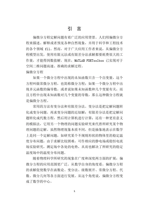
引言偏微分方程定解问题有着广泛的应用背景。
人们用偏微分方程来描述、解释或者预见各种自然现象,并用于科学和工程技术的各个领域fll。
然而,对于广大应用工作者来说,从偏微分方程模型出发,使用有限元法或有限差分法求解都要耗费很大的工作量,才能得到数值解。
现在,MATLAB PDEToolbox已实现对于空间二维问题高速、准确的求解过程。
偏微分方程如果一个微分方程中出现的未知函数只含一个自变量,这个方程叫做常微分方程,也简称微分方程;如果一个微分方程中出现多元函数的偏导数,或者说如果未知函数和几个变量有关,而且方程中出现未知函数对几个变量的导数,那么这种微分方程就是偏微分方程。
常用的方法有变分法和有限差分法。
变分法是把定解问题转化成变分问题,再求变分问题的近似解;有限差分法是把定解问题转化成代数方程,然后用计算机进行计算;还有一种更有意义的模拟法,它用另一个物理的问题实验研究来代替所研究某个物理问题的定解。
虽然物理现象本质不同,但是抽象地表示在数学上是同一个定解问题,如研究某个不规则形状的物体里的稳定温度分布问题,由于求解比较困难,可作相应的静电场或稳恒电流场实验研究,测定场中各处的电势,从而也解决了所研究的稳定温度场中的温度分布问题。
随着物理科学所研究的现象在广度和深度两方面的扩展,偏微分方程的应用范围更广泛。
从数学自身的角度看,偏微分方程的求解促使数学在函数论、变分法、级数展开、常微分方程、代数、微分几何等各方面进行发展。
从这个角度说,偏微分方程变成了数学的中心。
一、MATLAB方法简介及应用1.1 MATLAB简介MATLAB是美国MathWorks公司出品的商业数学软件,用于算法开发、数据可视化、数据分析以及数值计算的高级技术计算语言和交互式环境,主要包括MATLAB和Simulink两大部分。
1.2 Matlab主要功能数值分析数值和符号计算工程与科学绘图控制系统的设计与仿真数字图像处理数字信号处理通讯系统设计与仿真财务与金融工程1.3 优势特点1) 高效的数值计算及符号计算功能,能使用户从繁杂的数学运算分析中解脱出来;2) 具有完备的图形处理功能,实现计算结果和编程的可视化;3) 友好的用户界面及接近数学表达式的自然化语言,使学者易于学习和掌握;4) 功能丰富的应用工具箱(如信号处理工具箱、通信工具箱等) ,为用户提供了大量方便实用的处理工具。
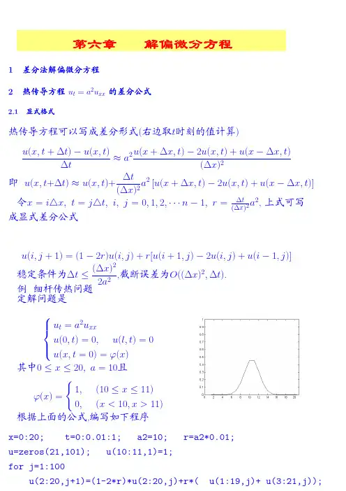
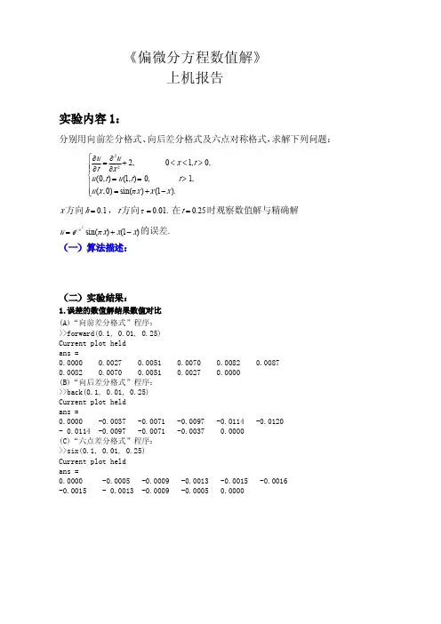
南京理工大学课程考核论文课程名称:高等数值分析论文题目:有限差分法求解偏微分方程*名:**学号:************成绩:有限差分法求解偏微分方程一、主要内容1.有限差分法求解偏微分方程,偏微分方程如一般形式的一维抛物线型方程:22(,)()u uf x t t xαα∂∂-=∂∂其中为常数具体求解的偏微分方程如下:22001(,0)sin()(0,)(1,)00u u x t x u x x u t u t t π⎧∂∂-=≤≤⎪∂∂⎪⎪⎪=⎨⎪⎪==≥⎪⎪⎩2.推导五种差分格式、截断误差并分析其稳定性;3.编写MATLAB 程序实现五种差分格式对偏微分方程的求解及误差分析;4.结论及完成本次实验报告的感想。
二、推导几种差分格式的过程:有限差分法(finite-difference methods )是一种数值方法通过有限个微分方程近似求导从而寻求微分方程的近似解。
有限差分法的基本思想是把连续的定解区域用有限个离散点构成的网格来代替;把连续定解区域上的连续变量的函数用在网格上定义的离散变量函数来近似;把原方程和定解条件中的微商用差商来近似,积分用积分和来近似,于是原微分方程和定解条件就近似地代之以代数方程组,即有限差分方程组,解此方程组就可以得到原问题在离散点上的近似解。
推导差分方程的过程中需要用到的泰勒展开公式如下:()2100000000()()()()()()()......()(())1!2!!n n n f x f x f x f x f x x x x x x x o x x n +'''=+-+-++-+- (2-1)求解区域的网格划分步长参数如下:11k k k kt t x x h τ++-=⎧⎨-=⎩ (2-2) 2.1 古典显格式2.1.1 古典显格式的推导由泰勒展开公式将(,)u x t 对时间展开得 2,(,)(,)()()(())i i k i k k k uu x t u x t t t o t t t∂=+-+-∂ (2-3) 当1k t t +=时有21,112,(,)(,)()()(())(,)()()i k i k i k k k k k i k i k uu x t u x t t t o t t tuu x t o tττ+++∂=+-+-∂∂=+⋅+∂ (2-4)得到对时间的一阶偏导数1,(,)(,)()=()i k i k i k u x t u x t uo t ττ+-∂+∂ (2-5) 由泰勒展开公式将(,)u x t 对位置展开得223,,21(,)(,)()()()()(())2!k i k i k i i k i i u uu x t u x t x x x x o x x x x∂∂=+-+-+-∂∂ (2-6)当11i i x x x x +-==和时,代入式(2-6)得2231,1,1122231,1,1121(,)(,)()()()()(())2!1(,)(,)()()()()(())2!i k i k i k i i i k i i i i i k i k i k i i i k i i i iu uu x t u x t x x x x o x x x x u u u x t u x t x x x x o x x x x ++++----⎧∂∂=+-+-+-⎪⎪∂∂⎨∂∂⎪=+-+-+-⎪∂∂⎩(2-7) 因为1k k x x h +-=,代入上式得2231,,22231,,21(,)(,)()()()2!1(,)(,)()()()2!i k i k i k i k i k i k i k i ku uu x t u x t h h o h x xu u u x t u x t h h o h x x +-⎧∂∂=+⋅+⋅+⎪⎪∂∂⎨∂∂⎪=-⋅+⋅+⎪∂∂⎩ (2-8) 得到对位置的二阶偏导数2211,22(,)2(,)(,)()()i k i k i k i k u x t u x t u x t u o h x h+--+∂=+∂ (2-9) 将式(2-5)、(2-9)代入一般形式的抛物线型偏微分方程得21112(,)(,)(,)2(,)(,)(,)()i k i k i k i k i k i k u x t u x t u x t u x t u x t f x t o h h αττ++---+⎡⎤-=++⎢⎥⎣⎦(2-10)为了方便我们可以将式(2-10)写成11122k kk k k k i i i i i i u u u u u f h ατ++-⎡⎤--+-=⎢⎥⎣⎦(2-11) ()11122k k kk k k i i i i i i u u uu u f h τατ++----+= (2-12)最后得到古典显格式的差分格式为()111(12)k k k k k i i i i i u ra u r u u f ατ++-=-+++ (2-13)2r h τ=其中,古典显格式的差分格式的截断误差是2()o h τ+。
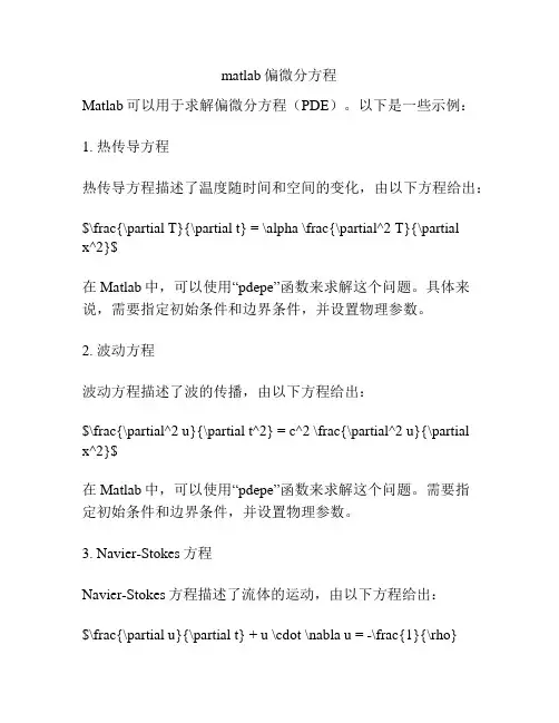
matlab偏微分方程Matlab可以用于求解偏微分方程(PDE)。
以下是一些示例:1. 热传导方程热传导方程描述了温度随时间和空间的变化,由以下方程给出:$\frac{\partial T}{\partial t} = \alpha \frac{\partial^2 T}{\partialx^2}$在Matlab中,可以使用“pdepe”函数来求解这个问题。
具体来说,需要指定初始条件和边界条件,并设置物理参数。
2. 波动方程波动方程描述了波的传播,由以下方程给出:$\frac{\partial^2 u}{\partial t^2} = c^2 \frac{\partial^2 u}{\partialx^2}$在Matlab中,可以使用“pdepe”函数来求解这个问题。
需要指定初始条件和边界条件,并设置物理参数。
3. Navier-Stokes方程Navier-Stokes方程描述了流体的运动,由以下方程给出:$\frac{\partial u}{\partial t} + u \cdot \nabla u = -\frac{1}{\rho}\nabla p + \nu \nabla^2 u$在Matlab中,可以使用PDE工具箱进行求解。
需要指定初始条件、边界条件和物理参数。
4. Schrödinger方程Schrödinger方程描述了量子力学中的波函数演化,由以下方程给出:$i \hbar \frac{\partial \psi}{\partial t} = -\frac{\hbar^2}{2m}\nabla^2 \psi + V(x) \psi$在Matlab中,可以使用PDE工具箱或ODE工具箱进行求解。
需要指定初始条件、边界条件和物理参数。
以上仅是部分示例,Matlab还可以用于求解其他类型的偏微分方程。
Matlab 偏微分方程求解方法目录:§1 Function Summary on page 10-87§2 Initial Value Problems on page 10-88§3 PDE Solver on page 10-89§4 Integrator Options on page 10-92§5 Examples” on page 10-93§1 Function Summary1.1 PDE Solver” on page 10-871,2 PDE Helper Functi on” on page 10-871.3 PDE SolverThis is the MATLAB PDE solver.PDE Helper Function§2 Initial Value Problemspdepe solves systems of parabolic and elliptic PDEs in one spatial variable x and time t, of the form)xu ,u ,t ,x (s ))x u ,u ,t ,x (f x (x x t u )x u ,u ,t ,x (c m m ∂∂+∂∂∂∂=∂∂∂∂- (10-2) The PDEs hold for b x a ,t t t f 0≤≤≤≤.The interval [a, b] must be finite. mcan be 0, 1, or 2, corresponding to slab, cylindrical, or spherical symmetry,respectively. If m > 0, thena ≥0 must also hold.In Equation 10-2,)x /u ,u ,t ,x (f ∂∂ is a flux term and )x /u ,u ,t ,x (s ∂∂ is a source term. The flux term must depend on x /u ∂∂. The coupling of the partial derivatives with respect to time is restricted to multiplication by a diagonal matrix )x /u ,u ,t ,x (c ∂∂. The diagonal elements of this matrix are either identically zero or positive. An element that is identically zero corresponds to an elliptic equation and otherwise to a parabolic equation. There must be at least one parabolic equation. An element of c that corresponds to a parabolic equation can vanish at isolated values of x if they are mesh points.Discontinuities in c and/or s due to material interfaces are permitted provided that a mesh point is placed at each interface.At the initial time t = t0, for all x the solution components satisfy initial conditions of the form)x (u )t ,x (u 00= (10-3)At the boundary x = a or x = b, for all t the solution components satisfy a boundary condition of the form0)xu ,u ,t ,x (f )t ,x (q )u ,t ,x (p =∂∂+ (10-4) q(x, t) is a diagonal matrix with elements that are either identically zero or never zero. Note that the boundary conditions are expressed in terms of the f rather than partial derivative of u with respect to x-x /u ∂∂. Also, ofthe two coefficients, only p can depend on u.§3 PDE Solver3.1 The PDE SolverThe MATLAB PDE solver, pdepe, solves initial-boundary value problems for systems of parabolic and elliptic PDEs in the one space variable x and time t.There must be at least one parabolic equation in the system.The pdepe solver converts the PDEs to ODEs using a second-order accurate spatial discretization based on a fixed set of user-specified nodes. The discretization method is described in [9]. The time integration is done with ode15s. The pdepe solver exploits the capabilities of ode15s for solving the differential-algebraic equations that arise when Equation 10-2 contains elliptic equations, and for handling Jacobians with a specified sparsity pattern. ode15s changes both the time step and the formula dynamically.After discretization, elliptic equations give rise to algebraic equations. If the elements of the initial conditions vector that correspond to elliptic equations are not “consistent” with the discretization, pdepe tries to adjust them before eginning the time integration. For this reason, the solution returned for the initial time may have a discretization error comparable to that at any other time. If the mesh is sufficiently fine, pdepe can find consistent initial conditions close to the given ones. If pdepe displays amessage that it has difficulty finding consistent initial conditions, try refining the mesh. No adjustment is necessary for elements of the initial conditions vector that correspond to parabolic equations.PDE Solver SyntaxThe basic syntax of the solver is:sol = pdepe(m,pdefun,icfun,bcfun,xmesh,tspan)Note Correspondences given are to terms used in “Initial Value Problems” on page 10-88.The input arguments arem: Specifies the symmetry of the problem. m can be 0 =slab, 1 = cylindrical, or 2 = spherical. It corresponds to m in Equation 10-2. pdefun: Function that defines the components of the PDE. Itcomputes the terms f,c and s in Equation 10-2, and has the form[c,f,s] = pdefun(x,t,u,dudx)where x and t are scalars, and u and dudx are vectors that approximate the solution and its partial derivative with respect to . c, f, and s are column vectors. c stores the diagonal elements of the matrix .icfun: Function that evaluates the initial conditions. It has the formu = icfun(x)When called with an argument x, icfun evaluates and returns the initial values of the solution components at x in the column vector u.bcfun:Function that evaluates the terms and of the boundary conditions. Ithas the form[pl,ql,pr,qr] = bcfun(xl,ul,xr,ur,t)where ul is the approximate solution at the left boundary xl = a and ur is the approximate solution at the right boundary xr = b. pl and ql are column vectors corresponding to p and the diagonal of q evaluated at xl. Similarly, pr and qr correspond to xr. When m>0 and a = 0, boundedness of the solution near x = 0 requires that the f vanish at a = 0. pdepe imposes this boundary condition automatically and it ignores values returned in pl and ql.xmesh:Vector [x0, x1, ..., xn] specifying the points at which a numerical solution is requested for every value in tspan. x0 and xn correspond to a and b , respectively. Second-order approximation to the solution is made on the mesh specified in xmesh. Generally, it is best to use closely spaced mesh points where the solution changes rapidly. pdepe does not select the mesh in automatically. You must provide an appropriate fixed mesh in xmesh. The cost depends strongly on the length of xmesh. When , it is not necessary to use a fine mesh near to x=0 account for the coordinate singularity.The elements of xmesh must satisfy x0 < x1 < ... < xn.The length of xmesh must be ≥3.tspan:Vector [t0, t1, ..., tf] specifying the points at which a solution is requested for every value in xmesh. t0 and tf correspond tot and f t,respectively.pdepe performs the time integration with an ODE solver that selects both the time step and formula dynamically. The solutions at the points specified in tspan are obtained using the natural continuous extension of the integration formulas. The elements of tspan merely specify where you want answers and the cost depends weakly on the length of tspan.The elements of tspan must satisfy t0 < t1 < ... < tf.The length of tspan must be ≥3.The output argument sol is a three-dimensional array, such that•sol(:,:,k) approximates component k of the solution .•sol(i,:,k) approximates component k of the solution at time tspan(i) and mesh points xmesh(:).•sol(i,j,k) approximates component k of the solution at time tspan(i) and the mesh point xmesh(j).4.2 PDE Solver OptionsFor more advanced applications, you can also specify as input arguments solver options and additional parameters that are passed to the PDE functions.options:Structure of optional parameters that change the default integration properties. This is the seventh input argument.sol = pdepe(m,pdefun,icfun,bcfun,xmesh,tspan,options)See “Integrator Options” on page 10-92 for more information.Integrator OptionsThe default integration properties in the MATLAB PDE solver are selected to handle common problems. In some cases, you can improve solver performance by overriding these defaults. You do this by supplying pdepe with one or more property values in an options structure.sol = pdepe(m,pdefun,icfun,bcfun,xmesh,tspan,options)Use odeset to create the options structure. Only those options of the underlying ODE solver shown in the following table are available for pdepe.The defaults obtained by leaving off the input argument options are generally satisfactory. “Integrator Options” on page 10-9 tells you how to create the structure and describes the properties.PDE Properties§4 Examples•“Single PDE” on page 10-93•“System of PDEs” on page 10-98•“Additional Examples” on page 10-1031.Single PDE• “Solving the Equation” on page 10-93• “Evaluating the Solution” on page 10-98Solving the Equation. This example illustrates the straightforward formulation, solution, and plotting of the solution of a single PDE222x u t u ∂∂=∂∂π This equation holds on an interval 1x 0≤≤ for times t ≥ 0. At 0t = the solution satisfies the initial condition x sin )0,x (u π=.At 0x =and 1x = , the solution satisfies the boundary conditions0)t ,1(xu e ,0)t ,0(u t =∂∂+π=- Note The demo pdex1 contains the complete code for this example. The demo uses subfunctions to place all functions it requires in a single MATLAB file.To run the demo type pdex1 at the command line. See “PDE Solver Syntax” on page 10-89 for more information. 1 Rewrite the PDE. Write the PDE in the form)xu ,u ,t ,x (s ))x u ,u ,t ,x (f x (x x t u )x u ,u ,t ,x (c m m ∂∂+∂∂∂∂=∂∂∂∂- This is the form shown in Equation 10-2 and expected by pdepe. For this example, the resulting equation is0x u x x x t u 002+⎪⎭⎫ ⎝⎛∂∂∂∂=∂∂π with parameter and the terms 0m = and the term0s ,xu f ,c 2=∂∂=π=2 Code the PDE. Once you rewrite the PDE in the form shown above (Equation 10-2) and identify the terms, you can code the PDE in a function that pdepe can use. The function must be of the form[c,f,s] = pdefun(x,t,u,dudx)where c, f, and s correspond to the f ,c and s terms. The code below computes c, f, and s for the example problem.function [c,f,s] = pdex1pde(x,t,u,DuDx)c = pi^2;f = DuDx;s = 0;3 Code the initial conditions function. You must code the initial conditions in a function of the formu = icfun(x)The code below represents the initial conditions in the function pdex1ic. Partial Differential Equationsfunction u0 = pdex1ic(x)u0 = sin(pi*x);4 Code the boundary conditions function. You must also code the boundary conditions in a function of the form[pl,ql,pr,qr] = bcfun(xl,ul,xr,ur,t) The boundary conditions, written in the same form as Equation 10-4, are0x ,0)t ,0(x u .0)t ,0(u ==∂∂+and1x ,0)t ,1(xu .1e t ==∂∂+π- The code below evaluates the components )u ,t ,x (p and )u ,t ,x (q of the boundary conditions in the function pdex1bc.function [pl,ql,pr,qr] = pdex1bc(xl,ul,xr,ur,t)pl = ul;ql = 0;pr = pi * exp(-t);qr = 1;In the function pdex1bc, pl and ql correspond to the left boundary conditions (x=0 ), and pr and qr correspond to the right boundary condition (x=1).5 Select mesh points for the solution. Before you use the MATLAB PDE solver, you need to specify the mesh points at which you want pdepe to evaluate the solution. Specify the points as vectors t and x.The vectors t and x play different roles in the solver (see “PDE Solver” on page 10-89). In particular, the cost and the accuracy of the solution depend strongly on the length of the vector x. However, the computation is much less sensitive to the values in the vector t.10 CalculusThis example requests the solution on the mesh produced by 20 equally spaced points from the spatial interval [0,1] and five values of t from thetime interval [0,2].x = linspace(0,1,20);t = linspace(0,2,5);6 Apply the PDE solver. The example calls pdepe with m = 0, the functions pdex1pde, pdex1ic, and pdex1bc, and the mesh defined by x and t at which pdepe is to evaluate the solution. The pdepe function returns the numerical solution in a three-dimensional array sol, wheresol(i,j,k) approximates the kth component of the solution,u, evaluated atkt(i) and x(j).m = 0;sol = pdepe(m,@pdex1pde,@pdex1ic,@pdex1bc,x,t);This example uses @ to pass pdex1pde, pdex1ic, and pdex1bc as function handles to pdepe.Note See the function_handle (@), func2str, and str2func reference pages, and the @ section of MATLAB Programming Fundamentals for information about function handles.7 View the results. Complete the example by displaying the results:a Extract and display the first solution component. In this example, the solution has only one component, but for illustrative purposes, the example “extracts” it from the three-dimensional array. The surface plot shows the behavior of the solution.u = sol(:,:,1);surf(x,t,u)title('Numerical solution computed with 20 mesh points') xlabel('Distance x') ylabel('Time t')Distance xNumerical solution computed with 20 mesh points.Time tb Display a solution profile at f t , the final value of . In this example,2t t f ==.figure plot(x,u(end,:)) title('Solution at t = 2') xlabel('Distance x') ylabel('u(x,2)')Solutions at t = 2.Distance xu (x ,2)Evaluating the Solution. After obtaining and plotting the solution above, you might be interested in a solution profile for a particular value of t, or the time changes of the solution at a particular point x. The kth column u(:,k)(of the solution extracted in step 7) contains the time history of the solution at x(k). The jth row u(j,:) contains the solution profile at t(j). Using the vectors x and u(j,:), and the helper function pdeval, you can evaluate the solution u and its derivative at any set of points xout [uout,DuoutDx] = pdeval(m,x,u(j,:),xout)The example pdex3 uses pdeval to evaluate the derivative of the solution at xout = 0. See pdeval for details.2. System of PDEsThis example illustrates the solution of a system of partial differential equations. The problem is taken from electrodynamics. It has boundary layers at both ends of the interval, and the solution changes rapidly for small . The PDEs are)u u (F xu017.0t u )u u (F xu 024.0t u 212222212121-+∂∂=∂∂--∂∂=∂∂ where )y 46.11exp()y 73.5exp()y (F --=. The equations hold on an interval1x 0≤≤ for times 0t ≥.The solution satisfies the initial conditions0)0,x (u ,1)0,x (u 21≡≡and boundary conditions0)t ,1(xu,0)t ,1(u ,0)t ,0(u ,0)t ,0(x u 2121=∂∂===∂∂ Note The demo pdex4 contains the complete code for this example. The demo uses subfunctions to place all required functions in a single MATLAB file. To run this example type pdex4 at the command line.1 Rewrite the PDE. In the form expected by pdepe, the equations are⎥⎦⎤⎢⎣⎡---+⎥⎦⎤⎢⎣⎡∂∂∂∂∂∂=⎥⎦⎤⎢⎣⎡∂∂⎥⎦⎤⎢⎣⎡)u u (F )u u (F )x /u 170.0)x /u (024.0x u u t *.1121212121 The boundary conditions on the partial derivatives of have to be written in terms of the flux. In the form expected by pdepe, the left boundary condition is⎥⎦⎤⎢⎣⎡=⎥⎦⎤⎢⎣⎡∂∂∂∂⎥⎦⎤⎢⎣⎡+⎥⎦⎤⎢⎣⎡00)x /u (170.0)x /u (024.0*.01u 0212and the right boundary condition is⎥⎦⎤⎢⎣⎡=⎥⎦⎤⎢⎣⎡∂∂∂∂⎥⎦⎤⎢⎣⎡+⎥⎦⎤⎢⎣⎡-00)x /u (170.0)x /u (024.0*.1001u 2112 Code the PDE. After you rewrite the PDE in the form shown above, you can code it as a function that pdepe can use. The function must be of the form[c,f,s] = pdefun(x,t,u,dudx)where c, f, and s correspond to the , , and terms in Equation 10-2. function [c,f,s] = pdex4pde(x,t,u,DuDx)c = [1; 1];f = [0.024; 0.17] .* DuDx;y = u(1) - u(2);F = exp(5.73*y)-exp(-11.47*y);s = [-F; F];3 Code the initial conditions function. The initial conditions function must be of the formu = icfun(x)The code below represents the initial conditions in the function pdex4ic. function u0 = pdex4ic(x);u0 = [1; 0];4 Code the boundary conditions function. The boundary conditions functions must be of the form[pl,ql,pr,qr] = bcfun(xl,ul,xr,ur,t)The code below evaluates the components p(x,t,u) and q(x,t) (Equation 10-4) of the boundary conditions in the function pdex4bc.function [pl,ql,pr,qr] = pdex4bc(xl,ul,xr,ur,t)pl = [0; ul(2)];ql = [1; 0];pr = [ur(1)-1; 0];qr = [0; 1];5 Select mesh points for the solution. The solution changes rapidly for small t . The program selects the step size in time to resolve this sharp change, but to see this behavior in the plots, output times must be selected accordingly. There are boundary layers in the solution at both ends of [0,1], so mesh points must be placed there to resolve these sharp changes. Often some experimentation is needed to select the mesh that reveals the behavior of the solution.x = [0 0.005 0.01 0.05 0.1 0.2 0.5 0.7 0.9 0.95 0.99 0.995 1];t = [0 0.005 0.01 0.05 0.1 0.5 1 1.5 2];6 Apply the PDE solver. The example calls pdepe with m = 0, the functions pdex4pde, pdex4ic, and pdex4bc, and the mesh defined by x and t at which pdepe is to evaluate the solution. The pdepe function returns the numerical solution in a three-dimensional array sol, wheresol(i,j,k) approximates the kth component of the solution, μk, evaluated at t(i) and x(j).m = 0;sol = pdepe(m,@pdex4pde,@pdex4ic,@pdex4bc,x,t);7 View the results. The surface plots show the behavior of the solution components. u1 = sol(:,:,1); u2 = sol(:,:,2); figure surf(x,t,u1) title('u1(x,t)') xlabel('Distance x') 其输出图形为Distance xu1(x,t)Time tfigure surf(x,t,u2) title('u2(x,t)') xlabel('Distance x') ylabel('Time t')Distance xu2(x,t)Time tAdditional ExamplesThe following additional examples are available. Type edit examplename to view the code and examplename to run the example.。
第四讲Matlab求解微分方程(组)理论介绍:Matlab求解微分方程(组)命令求解实例:Matlab求解微分方程(组)实例实际应用问题通过数学建模所归纳得到的方程,绝大多数都是微分方程,真正能得到代数方程的机会很少.另一方面,能够求解的微分方程也是十分有限的, 特别是高阶方程和偏微分方程(组).这就要求我们必须研究微分方程(组)的解法:解析解法和数值解法.一.相关函数、命令及简介1.在Matlab中,用大写字母D表示导数,Dy表示y关于自变量的一阶导数, D2y表示y关于自变量的二阶导数,依此类推.函数dsolve用来解决常微分方程(组)的求解问题,调用格式为:X=dsolve(<eqnl,,,eqn2函数dsolve用来解符号常微分方程、方程组,如果没有初始条件,则求出通解,如果有初始条件,则求出特解.注意,系统缺省的自变量为t2.函数dsolve求解的是常微分方程的精确解法,也称为常微分方程的符号解. 但是,有大量的常微分方程虽然从理论上讲,其解是存在的,但我们却无法求出其解析解,此时,我们需要寻求方程的数值解,在求常微分方程数值解方面,MATLAB具有丰富的函数,我们将其统称为solver,其一般格式为:[T,Y]=solver(odefun,tspan,yO)说明:(1 )solver 为命令ode45、ode23、odel 13、odel5s、ode23s、ode23t、ode23tb、odel5i 之一.(2)odefun是显示微分方程),=f (t,y)在积分区间tspan =[心心]上从心到“用初始条件儿求解.(3)如果要获得微分方程问题在其他指定时间点bG©…心上的解,则令(span = 『“,•••『/■](要单调的).(4)因为没有一种算法可以有效的解决所有的ODE问题,为此,Matlab提供T多种求解器solver,对于不同的ODE问题,采用不同的solver.程(组)的初值问题的解的Matlab常用程序,其中:ode23采用龙格-库塔2阶算法,用3阶公式作误差估计来调节步长,具有低等的精度.。
matlab解偏微分方程Matlab是一种非常强大的数学计算工具,它可以用于解决各种数学问题。
在本文中,我们将学习如何使用Matlab解偏微分方程。
偏微分方程是一类包含未知函数的偏导数的方程。
通常,解偏微分方程是困难的,需要使用复杂的数学方法。
然而,Matlab可以大大简化这个过程。
在Matlab中,我们可以使用pdepe函数来解偏微分方程。
pdepe函数采用一个偏微分方程的系统,并返回一个包含解的向量的矩阵。
下面是一个解二维扩散方程的示例程序:%定义二维扩散方程 function [c,f,s] = diffusionpde(x,t,u,DuDx)c = 1; %系数f = DuDx; %带有时间和空间导数的项s = 0; %不带导数的项end%定义边界条件(例)function [pl,ql,pr,qr] =diffusionbc(xl,ul,xr,ur,t)pl = 0; ql = 1; %左边界(u=0)pr = 0; qr = 1; %右边界(u=0)end%定义初始条件(例)function u0 = diffusionic(x)u0 = sin(pi*x); %sin(pi*x)是初始条件方程end%主程序x = linspace(0,1,50); %空间网格t = linspace(0,1,10); %时间网格sol =pdepe(0,@diffusionpde,@diffusionic,@diffusionbc,x,t );u = sol(:,:,1); %提取第一个解%绘制解surfc(x,t,u)xlabel('位置')ylabel('时间')title('二维扩散方程的解')从上述程序中,我们可以看到pdepe的使用方法。
在主程序中,我们选择了空间和时间网格,然后定义了偏微分方程、初始条件和边界条件的函数。
最后,我们调用pdepe函数,并将解存储在变量sol中。
MATLAB中的偏微分方程数值解法偏微分方程(Partial Differential Equations,PDEs)是数学中的重要概念,广泛应用于物理学、工程学、经济学等领域。
解决偏微分方程的精确解往往非常困难,因此数值方法成为求解这类问题的有效途径。
而在MATLAB中,有丰富的数值解法可供选择。
本文将介绍MATLAB中几种常见的偏微分方程数值解法,并通过具体案例加深对其应用的理解。
一、有限差分法(Finite Difference Method)有限差分法是最为经典和常用的偏微分方程数值解法之一。
它将偏微分方程的导数转化为差分方程,通过离散化空间和时间上的变量,将连续问题转化为离散问题。
在MATLAB中,使用有限差分法可以比较容易地实现对偏微分方程的数值求解。
例如,考虑一维热传导方程(Heat Equation):∂u/∂t = k * ∂²u/∂x²其中,u为温度分布随时间和空间的变化,k为热传导系数。
假设初始条件为一段长度为L的棒子上的温度分布,边界条件可以是固定温度、热交换等。
有限差分法可以将空间离散化为N个节点,时间离散化为M个时刻。
我们可以使用中心差分近似来计算二阶空间导数,从而得到以下差分方程:u(i,j+1) = u(i,j) + Δt * (k * (u(i+1,j) - 2 * u(i,j) + u(i-1,j))/Δx²)其中,i表示空间节点,j表示时间步。
Δt和Δx分别为时间和空间步长。
通过逐步迭代更新节点的温度值,我们可以得到整个时间范围内的温度分布。
而MATLAB提供的矩阵计算功能,可以大大简化有限差分法的实现过程。
二、有限元法(Finite Element Method)有限元法是另一种常用的偏微分方程数值解法,特点是适用于复杂的几何形状和边界条件。
它将求解区域离散化为多个小单元,通过构建并求解代数方程组来逼近连续问题。
在MATLAB中,我们可以使用Partial Differential Equation Toolbox提供的函数进行有限元法求解。

MATLAB学习(序列1)偏微分方程组的求解ode23 解非刚性微分方程,低精度,使用Runge-Kutta法的二三阶算法。
ode45 解非刚性微分方程,中等精度,使用Runge-Kutta法的四五阶算法。
ode113 解非刚性微分方程,变精度变阶次Adams-Bashforth-Moulton PECE算法。
ode23t 解中等刚性微分方程,使用自由内插法的梯形法则。
ode15s 解刚性微分方程,使用可变阶次的数值微分(NDFs)算法。
ode23s 解刚性微分方程,低阶方法,使用修正的Rosenbrock公式。
ode23tb 解刚性微分方程,低阶方法,使用TR-BDF2方法,即Runger-Kutta公式的第一级采用梯形法则,第二级采用Gear法。
[t,YY]=solver('F',tspan,Yo解算ODE初值问题的最简调用格式。
solver指上面的指令。
tspan=[0,30]; %时域t的范围y0=[1;0]; %y(1)y(2的初始值[tt,yy]=ode45(@DyDt,tspan,y0;plot(tt,yy(:,1,title('x(t'function ydot=DyDt(t,yydot=[y(2; 2*(1-y(1^2*y(2-y(1]刚性方程:刚性是指其Jacobian矩阵的特征值相差十分悬殊。
在解的性态上表现为,其中一些解变化缓慢,另一些变化快,且相差较悬殊,这类方程常常称为刚性方程,又称为Stiff方程。
刚性方程和非刚性方程对解法中步长选择的要求不同。
刚性方程一般不适合由ode45这类函数求解,而应该采用ode15s等。
如果不能分辨是否是刚性方程,先试用ode45,再用ode15s。
[t,YY,Te,Ye,Ie] = solver('F',tspan,Yo,options,p1,p2,…解算ODE初值问题的最完整调用格式。
为了能够解出方程,要用指令odeset确定求解的条件和要求。
精选全文完整版(可编辑修改)用差分法解椭圆型偏微分方程-(Uxx+Uyy)=(pi*pi-1)e^xsin(pi*y)0<x<2; 0<y<1U(0,y)=sin(pi*y),U(2,y)=e^2sin(pi*y); 0=<y<=1U(x,0)=0, U(x,1)=0;0=<x<=2先自己去看一下关于五点差分法的理论书籍Matlab程序:unction[p e u x y k]=wudianchafenfa(h,m,n,kmax,ep)% g-s迭代法解五点差分法问题%kmax为最大迭代次数%m,n为x,y方向的网格数,例如(2-0)/0.01=200;%e为误差,p为精确解symstemp;u=zeros(n+1,m+1);x=0+(0:m)*h;y=0+(0:n)*h;for(i=1:n+1)u(i,1)=sin(pi*y(i));u(i,m+1)=exp(1)*exp(1)*sin(pi*y(i));endfor(i=1:n)for(j=1:m)f(i,j)=(pi*pi-1)*exp(x(j))*sin(pi*y(i));endendt=zeros(n-1,m-1);for(k=1:kmax)for(i=2:n)for(j=2:m)temp=h*h*f(i,j)/4+(u(i,j+1)+u(i,j-1)+u(i+1,j)+u (i-1,j))/4;t(i,j)=(temp-u(i,j))*(temp-u(i,j));u(i,j)=temp;endendt(i,j)=sqrt(t(i,j));if(k>kmax)break;endif(max(max(t))<ep)break;endendfor(i=1:n+1)for(j=1:m+1)p(i,j)=exp(x(j))*sin(pi*y(i));e(i,j)=abs(u(i,j)-exp(x(j))*sin(pi*y(i)));endEnd在命令窗口中输入:[p e u xyk]=wudianchafenfa(0.1,20,10,10000,1e-6) k=147surf(x,y,u) ;xlabel(‘x’);ylabel(‘y’);zlabel(‘u’);Title(‘五点差分法解椭圆型偏微分方程例1’)就可以得到下图surf(x,y,p)surf(x,y,e)[p e uxy k]=wudianchafenfa(0.05,40,20,10000,1e-6)[pe u x y k]=wudianchafenfa(0.025,80,40,10000,1e-6)为什么分得越小,误差会变大呢?我们试试运行:[pe u x yk]=wudianchafenfa(0.025,80,40,10000,1e-8)K=2164surf(x,y,e)误差变小了吧还可以试试[p e ux y k]=wudianchafenfa(0.025,80,40,10000,1e-10) K=3355误差又大了一点再试试[peu x y k]=wudianchafenfa(0.025,80,40,10000,1e-11)k=3952 误差趋于稳定总结:最终的误差曲面与网格数有关,也与设定的迭代前后两次差值(ep,看程序)有关;固定网格数,随着设定的迭代前后两次差值变小,误差由大比变小,中间有一个最小值,随着又增大一点,最后趋于稳定。
Matlab 差分法解偏微分方程1.引言解偏微分方程是数学和工程领域中的一项重要课题,它在科学研究和工程实践中具有广泛的应用。
而 Matlab 差分法是一种常用的数值方法,用于求解偏微分方程。
本文将介绍 Matlab 差分法在解偏微分方程中的应用,包括原理、步骤和实例。
2. Matlab 差分法原理差分法是一种离散化求解微分方程的方法,通过近似替代微分项来求解微分方程的数值解。
在 Matlab 中,差分法可以通过有限差分法或者差分格式来实现。
有限差分法将微分方程中的导数用有限差分替代,而差分格式指的是使用不同的差分格式来近似微分方程中的各个项,通常包括前向差分、后向差分和中心差分等。
3. Matlab 差分法步骤使用 Matlab 差分法解偏微分方程一般包括以下步骤:(1)建立离散化的区域:将求解区域离散化为网格点或节点,并确定网格间距。
(2)建立离散化的时间步长:对于时间相关的偏微分方程,需要建立离散化的时间步长。
(3)建立离散化的微分方程:使用差分法将偏微分方程中的微分项转化为离散形式。
(4)建立迭代方程:根据离散化的微分方程建立迭代方程,求解数值解。
(5)编写 Matlab 代码:根据建立的迭代方程编写 Matlab 代码求解数值解。
(6)求解并分析结果:使用 Matlab 对建立的代码进行求解,并对结果进行分析和后处理。
4. Matlab 差分法解偏微分方程实例假设我们要使用 Matlab 差分法解决以下一维热传导方程:∂u/∂t = α * ∂^2u/∂x^2其中 u(x, t) 是热传导方程的温度分布,α 是热扩散系数。
4.1. 离散化区域和时间步长我们将求解区域离散化为网格点,分别为 x_i,i=1,2,...,N。
时间步长为Δt。
4.2. 离散化的微分方程使用中心差分格式将偏微分方程中的导数项离散化得到:∂u/∂t ≈ (u_i(t+Δt) - u_i(t))/Δt∂^2u/∂x^2 ≈ (u_i-1(t) - 2u_i(t) + u_i+1(t))/(Δx)^2代入原偏微分方程可得离散化的微分方程:(u_i(t+Δt) - u_i(t))/Δt = α * (u_i-1(t) - 2u_i(t) + u_i+1(t))/(Δx)^24.3. 建立迭代方程根据离散化的微分方程建立迭代方程:u_i(t+Δt) = u_i(t) + α * Δt * (u_i-1(t) - 2u_i(t) + u_i+1(t))/(Δx)^24.4. 编写 Matlab 代码使用以上建立的迭代方程编写 Matlab 代码求解热传导方程。
matlab 求解偏微分方程使用MATLAB求解偏微分方程摘要:偏微分方程(partial differential equation, PDE)是数学中重要的一类方程,广泛应用于物理、工程、经济、生物等领域。
MATLAB 是一种强大的数值计算软件,提供了丰富的工具箱和函数,可以用来求解各种类型的偏微分方程。
本文将介绍如何使用MATLAB来求解偏微分方程,并通过具体案例进行演示。
引言:偏微分方程是描述多变量函数的方程,其中包含了函数的偏导数。
一般来说,偏微分方程可以分为椭圆型方程、双曲型方程和抛物型方程三类。
求解偏微分方程的方法有很多,其中数值方法是最常用的一种。
MATLAB作为一种强大的数值计算软件,提供了丰富的工具箱和函数,可以用来求解各种类型的偏微分方程。
方法:MATLAB提供了多种求解偏微分方程的函数和工具箱,包括pdepe、pdetoolbox和pde模块等。
其中,pdepe函数是用来求解带有初始条件和边界条件的常微分方程组的函数,可以用来求解一维和二维的偏微分方程。
pdepe函数使用有限差分法或有限元法来离散化偏微分方程,然后通过求解离散化后的常微分方程组得到最终的解。
案例演示:考虑一维热传导方程的求解,偏微分方程为:∂u/∂t = α * ∂^2u/∂x^2其中,u(x,t)是温度分布函数,α是热扩散系数。
假设初始条件为u(x,0)=sin(pi*x),边界条件为u(0,t)=0和u(1,t)=0。
我们需要定义偏微分方程和边界条件。
在MATLAB中,可以使用匿名函数来定义偏微分方程和边界条件。
然后,我们使用pdepe函数求解偏微分方程。
```matlabfunction [c,f,s] = pde(x,t,u,DuDx)c = 1;f = DuDx;s = 0;endfunction u0 = uinitial(x)u0 = sin(pi*x);endfunction [pl,ql,pr,qr] = uboundary(xl,ul,xr,ur,t)pl = ul;ql = 0;pr = ur;qr = 0;endx = linspace(0,1,100);t = linspace(0,0.1,10);m = 0;sol = pdepe(m,@pde,@uinitial,@uboundary,x,t);u = sol(:,:,1);surf(x,t,u);xlabel('Distance x');ylabel('Time t');zlabel('Temperature u');```在上述代码中,我们首先定义了偏微分方程函数pde,其中c、f和s分别表示系数c、f和s。