英文版greene 计量经济学Ch9

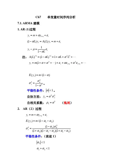
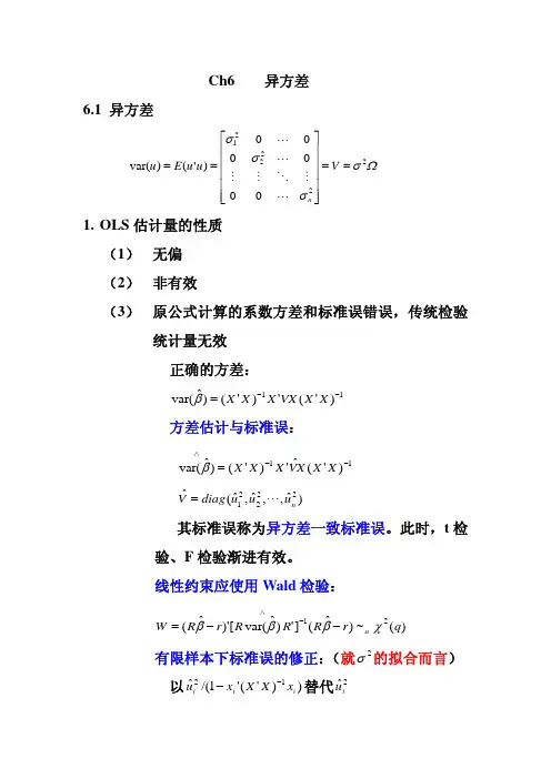
Ch7 单变量时间序列分析7.1. ARMA 建模 1. AR (1)过程t t t y m y εα++=−1t t t m y L A y L εα+==−)()1( t t Ly εαμ−=−11注： "+++=−=−−22111)1()(L L L L A ααα""+++++++=−−2212)1(t t t t m y εααεεαα)1/()(α−=m y E t2221ασσε−=y。

平稳性条件：1<α。

自协方差： 2y k kσαγ= 自相关系数： （拖尾）kk αρ=2. AR （2）过程t t t y m y εα++=−1 )1/()(21αα−−=m y E t)1)(1)(1()1(21212222ααααασασε−+−−+−=y 平稳性条件：（表述1） 12<α 121<+αα112<−αα Yule －Walker 方程： 自协方差： 12011γαγαγ+= 02112γαγαγ+= 自相关系数： 1211ρααρ+= 2112αραρ+=2111ααρ−=， 222121αααρ+−=22113−−>+=k k k ραραρ （拖尾） 滞后算子多项式的根：t t t m y L A y L L εαα+==−−)()1(221 )1)(1()(21L L L A λλ−−=24,221121αααλλ++=Ld L c L L L A 2121111)]1)(1/[(1)(λλλλ−+−=−−=−t t t t t Ld Lc x x y ελελμ212111−+−=+=−两个具有相同扰动的AR(1)过程的叠加。

特征方程：)(1221z A z z =−−αα 根：i i z λ/1= 平稳性条件：（表述2）11>z ，12>z如果出现复根，其模要小于1.即：特征方程的根位于单位园外。

第九章模型设定Model Specification and Diagnostic Testing1. Introduction假如模型没有被正确设定，我们会遇到model specification error或model specification bias 问题。

本章主要回答这些问题：1、选择模型的标准是什么？2、什么样的模型设定误差会经常遇到？3、模型设定误差的后果是什么？4、有那些诊断工具来发现模型设定误差？5、如果诊断有设定误差，如何校正，有何益处？6、怎样评估相互竞争模型的表现（model evaluation）？Model Selection Criteria这是笼统的模型选择标准：1、利用该模型进行预测在逻辑上是可能的；2、模型的参数具有稳定性，否则，预测就很困难。

弗里德曼说：模型有效性的唯一检验标准就是比较模型的预测是否与经验一致。

3、模型要与经济理论一致。

4、解释变量必须与误差项不相关。

5、模型的残差必须是白噪声；否则就存在模型设定误差。

6、最后选择的模型应该涵盖其它可能的竞争模型；也就是说，其他模型不应该比所选模型的表现更好。

Types of specification errors大概有这几种设定误差：设定误差之一：所选模型忽略了重要的解释变量（该解释变量被包含在模型误差中）设定误差之二：所选模型包含了不必要或不相关的解释变量设定误差之三：所选模型具有错误的方程形式（比如y采用了不该采用的对数转换）设定误差之四：被解释变量and/or解释变量测量偏差（所用数据相对于真实值有偏差）导致的误差（commit the errors of measurement bias）设定误差之五：随机误差项进入模型的形式不对引起的误差（比如是multiplicatively还是additively）The assumption of the CLRM that the econometric model is correctly specified has two meanings. One, there are no equation specification errors, and two, there are no model specification errors.上面概括的五种设定误差称为equation specification errors。

CHAPTER 1TEACHING NOTESYou have substantial latitude about what to emphasize in Chapter 1. I find it useful to talk about the economics of crime example (Example and the wage example (Example so that students see, at the outset, that econometrics is linked to economic reasoning, even if the economics is not complicated theory.I like to familiarize students with the important data structures that empirical economists use, focusing primarily on cross-sectional and time series data sets, as these are what I cover in a first-semester course. It is probably a good idea to mention the growing importance of data sets that have both a cross-sectional and time dimension.I spend almost an entire lecture talking about the problems inherent in drawing causal inferences in the social sciences. I do this mostly through the agricultural yield, return to education, and crime examples. These examples also contrast experimental and nonexperimental (observational) data. Students studying business and finance tend to find the term structure of interest rates example more relevant, although the issue there is testing the implication of a simple theory, as opposed to inferring causality. I have found that spending time talking about these examples, in place of a formal review of probability and statistics, is more successful (and more enjoyable for the students and me).CHAPTER 2TEACHING NOTESThis is the chapter where I expect students to follow most, if not all, of the algebraic derivations. In class I like to derive at least the unbiasedness of the OLS slope coefficient, and usually I derive the variance. At a minimum, I talk about the factors affecting the variance. To simplify the notation, after I emphasize the assumptions in the population model, and assume random sampling, I just condition on the values of the explanatory variables in the sample. Technically, this is justified by random sampling because, for example, E(u i|x1,x2,…,x n) = E(u i|x i) by independent sampling. I find that students are able to focus on the key assumption and subsequently take my word about how conditioning on the independent variables in the sample is harmless. (If you prefer, the appendix to Chapter 3 does the conditioning argument carefully.) Because statistical inference is no more difficult in multiple regression than in simple regression, I postpone inference until Chapter 4. (This reduces redundancy and allows you to focus on the interpretive differences between simple and multiple regression.)You might notice how, compared with most other texts, I use relatively few assumptions to derive the unbiasedness of the OLS slope estimator, followed by the formula for its variance. This is because I do not introduce redundant or unnecessary assumptions. For example, once is assumed, nothing further about the relationship between u and x is needed to obtain the unbiasedness of OLS under random sampling.CHAPTER 3TEACHING NOTESFor undergraduates, I do not work through most of the derivations in this chapter, at least not in detail. Rather, I focus on interpreting the assumptions, which mostly concern the population. Other than random sampling, the only assumption that involves more than population considerations is the assumption about no perfect collinearity, where the possibility of perfect collinearity in the sample (even if it does not occur in the population) should be touched on. The more important issue is perfect collinearity in the population, but this is fairly easy to dispense with via examples. These come from my experiences with the kinds of model specification issues that beginners have trouble with.The comparison of simple and multiple regression estimates – based on the particular sample at hand, as opposed to their statistical properties?– usually makes a strong impression. Sometimes I do not bother with the “partialling out” interpretation of multiple regression.As far as statistical properties, notice how I treat the problem of including an irrelevant variable: no separate derivation is needed, as the result follows form Theorem .I do like to derive the omitted variable bias in the simple case. This is not much more difficult than showing unbiasedness of OLS in the simple regression case under the first four Gauss-Markov assumptions. It is important to get the students thinking about this problem early on, and before too many additional (unnecessary) assumptions have been introduced.I have intentionally kept the discussion of multicollinearity to a minimum. This partly indicates my bias, but it also reflects reality. It is, of course, very important for students to understand the potential consequences of having highly correlated independent variables. But this is often beyond our control, except that we can ask less of our multiple regression analysis. If two or more explanatory variables are highly correlated in the sample, we should not expect to precisely estimate their ceteris paribus effects in the population.I find extensive treatmen ts of multicollinearity, where one “tests” or somehow “solves” the multicollinearity problem, to be misleading, at best. Even the organization of some texts gives the impression that imperfect multicollinearity is somehow a violation of the Gauss-Markov assumptions: they include multicollinearity in a chapter or part of the book devoted to “violation of the basic assumptions,” or something like that. I have noticed that master’s students who have had some undergraduate econometrics are often confused on the multicollinearity issue. It is very important that students not confuse multicollinearity among the included explanatory variables in a regression model with the bias caused by omitting an important variable.I do not prove the Gauss-Markov theorem. Instead, I emphasize its implications. Sometimes, and certainly for advanced beginners, I put a special case of Problem on a midterm exam, where I make a particular choice for the functiong(x). Rather than have the students directly compare the variances, they shouldappeal to the Gauss-Markov theorem for the superiority of OLS over any other linear, unbiased estimator.CHAPTER 4TEACHING NOTESAt the start of this chapter is good time to remind students that a specific error distribution played no role in the results of Chapter 3. That is because only the first two moments were derived under the full set of Gauss-Markov assumptions. Nevertheless, normality is needed to obtain exact normal sampling distributions (conditional on the explanatory variables). I emphasize that the full set of CLM assumptions are used in this chapter, but that in Chapter 5 we relax the normality assumption and still perform approximately valid inference. One could argue that the classical linear model results could be skipped entirely, and that only large-sample analysis is needed. But, from a practical perspective, students still need to know where the t distribution comes from because virtually all regression packages report t statistics and obtain p -values off of the t distribution. I then find it very easy tocover Chapter 5 quickly, by just saying we can drop normality and still use t statistics and the associated p -values as being approximately valid. Besides, occasionally students will have to analyze smaller data sets, especially if they do their own small surveys for a term project.It is crucial to emphasize that we test hypotheses about unknown population parameters. I tell my students that they will be punished if they write something likeH 0:1ˆ ?= 0 on an exam or, even worse, H 0: .632 = 0. One useful feature of Chapter 4 is its illustration of how to rewrite a population model so that it contains the parameter of interest in testing a single restriction. I find this is easier, both theoretically and practically, than computing variances that can, in some cases, depend on numerous covariance terms. The example of testing equality of the return to two- and four-year colleges illustrates the basic method, and shows that the respecified model can have a useful interpretation. Of course, some statistical packages now provide a standard error for linear combinations of estimates with a simple command, and that should be taught, too.One can use an F test for single linear restrictions on multiple parameters, but this is less transparent than a t test and does not immediately produce the standard error needed for a confidence interval or for testing a one-sided alternative. The trick of rewriting the population model is useful in several instances, including obtaining confidence intervals for predictions in Chapter 6, as well as for obtaining confidence intervals for marginal effects in models with interactions (also in Chapter6).The major league baseball player salary example illustrates the differencebetween individual and joint significance when explanatory variables (rbisyr and hrunsyr in this case) are highly correlated. I tend to emphasize the R -squared form of the F statistic because, in practice, it is applicable a large percentage of the time, and it is much more readily computed. I do regret that this example is biased toward students in countries where baseball is played. Still, it is one of the better examplesof multicollinearity that I have come across, and students of all backgrounds seem to get the point.CHAPTER 5TEACHING NOTESChapter 5 is short, but it is conceptually more difficult than the earlier chapters, primarily because it requires some knowledge of asymptotic properties of estimators. In class, I give a brief, heuristic description of consistency and asymptotic normality before stating the consistency and asymptotic normality of OLS. (Conveniently, the same assumptions that work for finite sample analysis work for asymptotic analysis.) More advanced students can follow the proof of consistency of the slope coefficient in the bivariate regression case. Section contains a full matrix treatment of asymptoti c analysis appropriate for a master’s level course.An explicit illustration of what happens to standard errors as the sample size grows emphasizes the importance of having a larger sample. I do not usually cover the LM statistic in a first-semester course, and I only briefly mention the asymptotic efficiency result. Without full use of matrix algebra combined with limit theorems for vectors and matrices, it is very difficult to prove asymptotic efficiency of OLS.I think the conclusions of this chapter are important for students to know, even though they may not fully grasp the details. On exams I usually include true-false type questions, with explanation, to test the students’ understanding of asymptotics. [For exam ple: “In large samples we do not have to worry about omitted variable bias.” (False). Or “Even if the error term is not normally distributed, in large samples we can still compute approximately valid confidence intervals under the Gauss-Markov assumptio ns.” (True).]CHAPTER6TEACHING NOTESI cover most of Chapter 6, but not all of the material in great detail. I use the example in Table to quickly run through the effects of data scaling on the important OLS statistics. (Students should already have a feel for the effects of data scaling on the coefficients, fitting values, and R-squared because it is covered in Chapter 2.) At most, I briefly mention beta coefficients; if students have a need for them, they can read this subsection.The functional form material is important, and I spend some time on more complicated models involving logarithms, quadratics, and interactions. An important point for models with quadratics, and especially interactions, is that we need to evaluate the partial effect at interesting values of the explanatory variables. Often, zero is not an interesting value for an explanatory variable and is well outside the range in the sample. Using the methods from Chapter 4, it is easy to obtain confidence intervals for the effects at interesting x values.As far as goodness-of-fit, I only introduce the adjusted R-squared, as I think using a slew of goodness-of-fit measures to choose a model can be confusing to novices (and does not reflect empirical practice). It is important to discuss how, if we fixate on a high R-squared, we may wind up with a model that has no interesting ceteris paribus interpretation.I often have students and colleagues ask if there is a simple way to predict y when log(y) has been used as the dependent variable, and to obtain a goodness-of-fit measure for the log(y) model that can be compared with the usual R-squared obtained when y is the dependent variable. The methods described in Section are easy to implement and, unlike other approaches, do not require normality.The section on prediction and residual analysis contains several important topics, including constructing prediction intervals. It is useful to see how much wider the prediction intervals are than the confidence interval for the conditional mean. I usually discuss some of the residual-analysis examples, as they have real-world applicability.CHAPTER 7TEACHING NOTESThis is a fairly standard chapter on using qualitative information in regression analysis, although I try to emphasize examples with policy relevance (and only cross-sectional applications are included.).In allowing for different slopes, it is important, as in Chapter 6, to appropriately interpret the parameters and to decide whether they are of direct interest. For example, in the wage equation where the return to education is allowed to depend on gender, the coefficient on the female dummy variable is the wage differential between women and men at zero years of education. It is not surprising that we cannot estimate this very well, nor should we want to. In this particular example we would drop the interaction term because it is insignificant, but the issue of interpreting the parameters can arise in models where the interaction term is significant.In discussing the Chow test, I think it is important to discuss testing for differences in slope coefficients after allowing for an intercept difference. In many applications, a significant Chow statistic simply indicates intercept differences. (See the example in Section on student-athlete GPAs in the text.) From a practical perspective, it is important to know whether the partial effects differ across groups or whether a constant differential is sufficient.I admit that an unconventional feature of this chapter is its introduction of the linear probability model. I cover the LPM here for several reasons. First, the LPM is being used more and more because it is easier to interpret than probit or logit models. Plus, once the proper parameter scalings are done for probit and logit, the estimated effects are often similar to the LPM partial effects near the mean or median values of the explanatory variables. The theoretical drawbacks of the LPM are often of secondary importance in practice. Computer Exercise is a good one to illustrate that, even with over 9,000 observations, the LPM can deliver fitted values strictly between zero and one for all observations.If the LPM is not covered, many students will never know about using econometrics to explain qualitative outcomes. This would be especially unfortunate for students who might need to read an article where an LPM is used, or who might want to estimate an LPM for a term paper or senior thesis. Once they are introduced to purpose and interpretation of the LPM, along with its shortcomings, they can tackle nonlinear models on their own or in a subsequent course.A useful modification of the LPM estimated in equation is to drop kidsge6 (because it is not significant) and then define two dummy variables, one for kidslt6 equal to one and the other for kidslt6 at least two. These can be included in place of kidslt6 (with no young children being the base group). This allows a diminishing marginal effect in an LPM. I was a bit surprised when a diminishing effect did not materialize.CHAPTER 8TEACHING NOTESThis is a good place to remind students that homoskedasticity played no role in showing that OLS is unbiased for the parameters in the regression equation. In addition, you probably should mention that there is nothing wrong with the R-squared or adjusted R-squared as goodness-of-fit measures. The key is that these are estimates of the population R-squared, 1?– [Var(u)/Var(y)], where the variances are the unconditional variances in the population. The usual R-squared, and the adjusted version, consistently estimate the population R-squared whether or not Var(u|x)?= Var(y|x) depends on x. Of course, heteroskedasticity causes the usual standard errors, t statistics, and F statistics to be invalid, even in large samples, with or without normality.By explicitly stating the homoskedasticity assumption as conditional on the explanatory variables that appear in the conditional mean, it is clear that only heteroskedasticity that depends on the explanatory variables in the model affects the validity of standard errors and test statistics. The version of the Breusch-Pagan test in the text, and the White test, are ideally suited for detecting forms of heteroskedasticity that invalidate inference obtained under homoskedasticity. If heteroskedasticity depends on an exogenous variable that does not also appear in the mean equation, this can be exploited in weighted least squares for efficiency, but only rarely is such a variable available. One case where such a variable is available is when an individual-level equation has been aggregated. I discuss this case in the text but I rarely have time to teach it.As I mention in the text, other traditional tests for heteroskedasticity, such as the Park and Glejser tests, do not directly test what we want, or add too many assumptions under the null. The Goldfeld-Quandt test only works when there is a natural way to order the data based on one independent variable. This is rare in practice, especially for cross-sectional applications.Some argue that weighted least squares estimation is a relic, and is no longer necessary given the availability of heteroskedasticity-robust standard errors and test statistics. While I am sympathetic to this argument, it presumes that we do not care much about efficiency. Even in large samples, the OLS estimates may not be preciseenough to learn much about the population parameters. With substantial heteroskedasticity we might do better with weighted least squares, even if the weighting function is misspecified. As discussed in the text on pages 288-289, one can, and probably should, compute robust standard errors after weighted least squares. For asymptotic efficiency comparisons, these would be directly comparable to the heteroskedasiticity-robust standard errors for OLS.Weighted least squares estimation of the LPM is a nice example of feasible GLS, at least when all fitted values are in the unit interval. Interestingly, in the LPM examples in the text and the LPM computer exercises, the heteroskedasticity-robust standard errors often differ by only small amounts from the usual standard errors. However, in a couple of cases the differences are notable, as in Computer Exercise .CHAPTER 9TEACHING NOTESThe coverage of RESET in this chapter recognizes that it is a test for neglected nonlinearities, and it should not be expected to be more than that. (Formally, it can be shown that if an omitted variable has a conditional mean that is linear in the included explanatory variables, RESET has no ability to detect the omitted variable. Interested readers may consult my chapter in Companion to Theoretical Econometrics, 2001, edited by Badi Baltagi.) I just teach students the F statistic version of the test.The Davidson-MacKinnon test can be useful for detecting functional form misspecification, especially when one has in mind a specific alternative, nonnested model. It has the advantage of always being a one degree of freedom test.I think the proxy variable material is important, but the main points can be made with Examples and . The first shows that controlling for IQ can substantially change the estimated return to education, and the omitted ability bias is in the expected direction. Interestingly, education and ability do not appear to have an interactive effect. Example is a nice example of how controlling for a previous value of the dependent variable – something that is often possible with survey and nonsurvey data – can greatly affect a policy conclusion. Computer Exercise is also a good illustration of this method.I rarely get to teach the measurement error material, although the attenuation bias result for classical errors-in-variables is worth mentioning.The result on exogenous sample selection is easy to discuss, with more details given in Chapter 17. The effects of outliers can be illustrated using the examples. I think the infant mortality example, Example , is useful for illustrating how a single influential observation can have a large effect on the OLS estimates.With the growing importance of least absolute deviations, it makes sense to at least discuss the merits of LAD, at least in more advanced courses. Computer Exercise is a good example to show how mean and median effects can be very different, even though there may not be “outliers” in the usual sense.CHAPTER 10TEACHING NOTESBecause of its realism and its care in stating assumptions, this chapter puts a somewhat heavier burden on the instructor and student than traditional treatments of time series regression. Nevertheless, I think it is worth it. It is important that students learn that there are potential pitfalls inherent in using regression with time series data that are not present for cross-sectional applications. Trends, seasonality, and high persistence are ubiquitous in time series data. By this time, students should have a firm grasp of multiple regression mechanics and inference, and so you can focus on those features that make time series applications different fromcross-sectional ones.I think it is useful to discuss static and finite distributed lag models at the same time, as these at least have a shot at satisfying the Gauss-Markov assumptions.Many interesting examples have distributed lag dynamics. In discussing the time series versions of the CLM assumptions, I rely mostly on intuition. The notion of strict exogeneity is easy to discuss in terms of feedback. It is also pretty apparent that, in many applications, there are likely to be some explanatory variables that are not strictly exogenous. What the student should know is that, to conclude that OLS is unbiased – as opposed to consistent – we need to assume a very strong form of exogeneity of the regressors. Chapter 11 shows that only contemporaneous exogeneity is needed for consistency.Although the text is careful in stating the assumptions, in class, after discussing strict exogeneity, I leave the conditioning on X implicit, especially when I discuss the no serial correlation assumption. As this is a new assumption I spend some time on it. (I also discuss why we did not need it for random sampling.)Once the unbiasedness of OLS, the Gauss-Markov theorem, and the sampling distributions under the classical linear model assumptions have been covered – which can be done rather quickly – I focus on applications. Fortunately, the students already know about logarithms and dummy variables. I treat index numbers in this chapter because they arise in many time series examples.A novel feature of the text is the discussion of how to compute goodness-of-fit measures with a trending or seasonal dependent variable. While detrending or deseasonalizing y is hardly perfect (and does not work with integrated processes), it is better than simply reporting the very high R-squareds that often come with time series regressions with trending variables.CHAPTER 11TEACHING NOTESMuch of the material in this chapter is usually postponed, or not covered at all, in an introductory course. However, as Chapter 10 indicates, the set of time series applications that satisfy all of the classical linear model assumptions might be very small. In my experience, spurious time series regressions are the hallmark of many student projects that use time series data. Therefore, students need to be alerted to the dangers of using highly persistent processes in time series regression equations.(Spurious regression problem and the notion of cointegration are covered in detail in Chapter 18.)It is fairly easy to heuristically describe the difference between a weakly dependent process and an integrated process. Using the MA(1) and the stable AR(1) examples is usually sufficient.When the data are weakly dependent and the explanatory variables are contemporaneously exogenous, OLS is consistent. This result has many applications, including the stable AR(1) regression model. When we add the appropriate homoskedasticity and no serial correlation assumptions, the usual test statistics are asymptotically valid.The random walk process is a good example of a unit root (highly persistent) process. In a one-semester course, the issue comes down to whether or not to first difference the data before specifying the linear model. While unit root tests are covered in Chapter 18, just computing the first-order autocorrelation is often sufficient, perhaps after detrending. The examples in Section illustrate how different first-difference results can be from estimating equations in levels.Section is novel in an introductory text, and simply points out that, if a modelis dynamically complete in a well-defined sense, it should not have serial correlation. Therefore, we need not worry about serial correlation when, say, we test the efficient market hypothesis. Section further investigates the homoskedasticity assumption, and, in a time series context, emphasizes that what is contained in the explanatory variables determines what kind of heteroskedasticity is ruled out by the usual OLS inference. These two sections could be skipped without loss of continuity.CHAPTER 12TEACHING NOTESMost of this chapter deals with serial correlation, but it also explicitly considers heteroskedasticity in time series regressions. The first section allows a review of what assumptions were needed to obtain both finite sample and asymptotic results. Just as with heteroskedasticity, serial correlation itself does not invalidate R-squared. In fact, if the data are stationary and weakly dependent, R-squared and adjustedR-squared consistently estimate the population R-squared (which is well-defined under stationarity).Equation is useful for explaining why the usual OLS standard errors are not generally valid with AR(1) serial correlation. It also provides a good starting point for discussing serial correlation-robust standard errors in Section . The subsection on serial correlation with lagged dependent variables is included to debunk the myth that OLS is always inconsistent with lagged dependent variables and serial correlation.I do not teach it to undergraduates, but I do to master’s students.Section is somewhat untraditional in that it begins with an asymptotic t testfor AR(1) serial correlation (under strict exogeneity of the regressors). It may seem heretical not to give the Durbin-Watson statistic its usual prominence, but I do believe the DW test is less useful than the t test. With nonstrictly exogenous regressors Icover only the regression form of Durbin’s test, as the h statistic is asymptotically equivalent and not always computable.Section , on GLS and FGLS estimation, is fairly standard, although I try to show how comparing OLS estimates and FGLS estimates is not so straightforward. Unfortunately, at the beginning level (and even beyond), it is difficult to choose a course of action when they are very different.I do not usually cover Section in a first-semester course, but, because some econometrics packages routinely compute fully robust standard errors, students can be pointed to Section if they need to learn something about what the corrections do. I do cover Section for a master’s level course in applied econometrics (after thefirst-semester course).I also do not cover Section in class; again, this is more to serve as a reference for more advanced students, particularly those with interests in finance. One important point is that ARCH is heteroskedasticity and not serial correlation, something that is confusing in many texts. If a model contains no serial correlation, the usual heteroskedasticity-robust statistics are valid. I have a brief subsection on correcting for a known form of heteroskedasticity and AR(1) errors in models with strictly exogenous regressors.CHAPTER 13TEACHING NOTESWhile this chapter falls under “Advanced Topics,” most of this chapter requires no more sophistication than the previous chapters. (In fact, I would argue that, with the possible exception of Section , this material is easier than some of the time series chapters.)Pooling two or more independent cross sections is a straightforward extension of cross-sectional methods. Nothing new needs to be done in stating assumptions, except possibly mentioning that random sampling in each time period is sufficient. The practically important issue is allowing for different intercepts, and possibly different slopes, across time.The natural experiment material and extensions of the difference-in-differences estimator is widely applicable and, with the aid of the examples, easy to understand.Two years of panel data are often available, in which case differencing across time is a simple way of removing g unobserved heterogeneity. If you have covered Chapter 9, you might compare this with a regression in levels using the second year of data, but where a lagged dependent variable is included. (The second approach only requires collecting information on the dependent variable in a previous year.) These often give similar answers. Two years of panel data, collected before and after a policy change, can be very powerful for policy analysis.Having more than two periods of panel data causes slight complications in that the errors in the differenced equation may be serially correlated. (However, the traditional assumption that the errors in the original equation are serially uncorrelated is not always a good one. In other words, it is not always more appropriate to used。

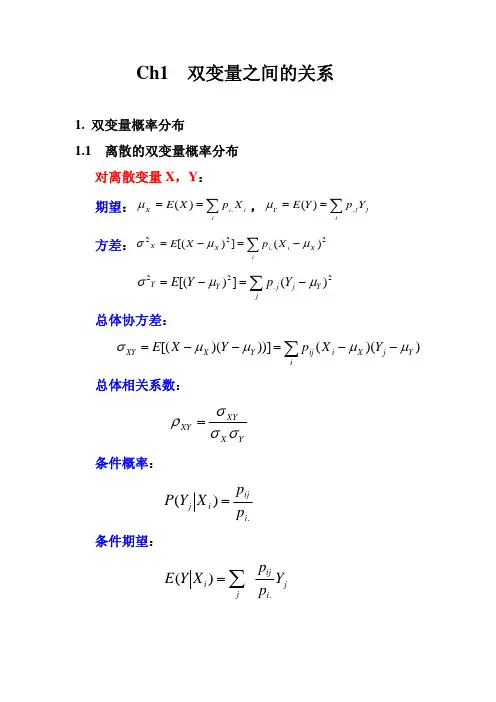
第一章1.Econometrics（计量经济学）：the social science in which the tools of economic theory，mathematics, and statistical inference are applied to the analysis of economic phenomena。

the result of a certain outlook on the role of economics，consists of the application of mathematical statistics to economic data to lend empirical support to the models constructed by mathematical economics and to obtain numerical results。

2.Econometric analysis proceeds along the following lines计量经济学分析步骤1)Creating a statement of theory or hypothesis。

建立一个理论假说2)Collecting data.收集数据3)Specifying the mathematical model of theory。

设定数学模型4)Specifying the statistical, or econometric，model of theory.设立统计或经济计量模型5)Estimating the parameters of the chosen econometric model.估计经济计量模型参数6)Checking for model adequacy : Model specification testing.核查模型的适用性：模型设定检验7)Testing the hypothesis derived from the model。

Ch3 多元回归方程1. 多元回归的矩阵表述u +βX Y ＝正规方程：YX X 'ˆX)'(=β或0ˆ'=uX OLS ：Y X X X ''ˆ1−=）（β21')ˆvar(σβ−=）（X X 1.1多元回归的离差形式 取离差矩阵：对称幂等矩阵'1ii nI A n −=)'1,,1("=i'1ii n取均值矩阵 回归方程u ˆˆX Y +β＝ uX AX uA A ˆˆˆ]0[ˆˆX AY 212+⎟⎟⎠⎞⎜⎜⎝⎛=+βββ＝ （u u =A ，0A =i ）u AX ˆˆAY 22+β＝1.2方差分解u u AX A X u AX u AX ˆ'ˆ'ˆ)ˆˆ()'ˆˆ((AY)(AY)'22''222222+=++ββββ＝ TSS ＝ ESS ＋ RSS 信息准则：，TSS/RSS 1R 2−＝)1/()/(RSS 1R 2−−−n TSS k n ＝， nkn AIC 2RSS ln +＝，n nkn SC ln RSS ln +＝，1.3偏相关系数i i i u X X +++33221i Y βββ＝一阶偏相关系数)1)(1(ˆˆˆˆ22321323131223.223.13.23.112.3γγγγγ−−−=∑∑∑r u uu u＝判定系数：）－（＋＝21222.1312223.121Rγγγ复相关系数的含义？ 231R 。

解释变量解释能力的分解问题：解释变量之间不相关：21312223.12R γγ＋＝ 解释变量相关：（1） K ruskal 法：简单相关系数和偏相关系数平方和的均值。

如：（）/2。

（各变量贡献的总和不为1） 23.12122γγ＋（2） Tinbergen 图：比较各变量乘以系数后的变异。

1.4复回归系数 u ˆˆX Y +β＝MY Y X X X X Y X Y u=−=−=')'(ˆˆβ 求残差矩阵：对称幂等矩阵')'(X X X X I M −=且： 0=MX u uM ˆˆ= 回归方程离差形式：u X X Y ˆˆˆ][*2*2+⎥⎥⎦⎤⎢⎢⎣⎡=ββ 令')'(*****X X X X I M −= u X M u M X X M Y M ˆˆˆˆˆ][22***2*2**+=+⎥⎥⎦⎤⎢⎢⎣⎡=βββ () 22*2*2ˆβX M X Y M X =Y M X X M X *212*22)(ˆ−=β 与偏相关系数的关系：2*2*k 3.122''ˆX M X YM Y ～。

计量经济学格林计量经济学格林是一种经济分析方法，它以经济数据为基础，运用统计学、经济理论和计算机技术等多种工具，对经济现象进行预测、评估和解释。

1. 什么是计量经济学格林？计量经济学格林指的是对经济模型进行参数估计的方法。

它的主要思想是运用多元回归模型，寻找不同变量之间的关系，并进行参数估计，可以衡量不同变量对经济变化的影响程度。

在经济领域，格林常常被用来估计市场需求、生产成本等因素对价格的影响。

2. 计量经济学格林的应用（1）市场需求估计市场需求是指一种商品或服务在市场上的购买量，将市场需求量作为因变量，商品价格、所得水平等交易因素作为自变量运用多元回归分析方法，可以得出商品价格弹性和收入弹性等关键参数。

（2）生产成本估计生产成本是指制造一个商品所需的资源投入，在这个参数估计中，将产品价格作为因变量，产品的许多生产成本指标作为自变量，如劳动力成本、制造成本等，估计商品生产的最低成本或最大利润点。

（3）风险分析与预测通过历史数据的分析，以及通过实际风险的评估，可以使用计量经济学格林的方法，预测未来的经济事件。

这种预测可以帮助企业、政府等做好合理的决策。

3. 计量经济学格林的限制计量经济学格林的参数估计依赖于建立模型的假设，模型本身的偏差会影响参数估计的准确性。

如果经济模型没有完全反映出主要因素和影响因素，那么格林分析将会受到制约。

此外，计量经济学格林还没有涵盖所有的人类经济活动，例如生态环境、文化背景等因素都没有被充分分析。

4. 结论计量经济学格林是一种有限的计量模型，它的应用范围也有限。

但是，将其与其他经济理论和方法相结合，可以得到更为精准的经济分析结果。

因此，在具体应用的时候，要多方面地考虑，运用多种不同的方法进行经济研究。