LS-DYNA中的能量平衡
- 格式:pdf
- 大小:286.54 KB
- 文档页数:6
HyperMesh&LS-DYNA控制卡片目录一.控制卡片 (1)二.控制卡片使用原则 (1)三.控制卡片的建立 (1)四.控制卡片参数说明 (2)*CONTROL_BULK_VISCOSITY(体积粘度控制) (2)*CONTROL_CONTACT(接触控制) (2)*CONTROL_CPU(CPU时间控制) (4)*CONTROL_ENERGY(能量耗散控制) (4)*CONTROL_HOURGLASS(沙漏控制) (4)*CONTROL_SHELL(单元控制) (5)*CONTROL_TERMINATION(计算终止控制卡片) (7)*CONTROL_TIMESTEP(时间步长控制卡片) (7)*DATABASE_BINARY_D3PLOT(完全输出控制) (9)*DATABASE_BINARY_D3THDT (10)*DATABASE_BINARY_INTFOR(接触面二进制数据输出控制) (10)*DATABASE_EXTENT_BINARY(输出数据控制) (10)*DATABASE_OPTION(指定输出文件) (12)*CONTROL_OUTPUT (15)*CONTROL_DYNAMIC_RELAXATION(动力释放) (16)*DATABASE_BINARY_OPTION(二进制文件的输出设置) (17)一.控制卡片碰撞分析控制卡片包括求解控制和结果输出控制,其中*KEYWORD、*CONTROL_TERMINATION、*DATABASE_BINARY_D3PLOT是必不可少的。
其他一些控制卡片如沙漏能控制、时间步控制、接触控制等则对计算过程进行控制,以便在发现模型中存在错误时及时的终止程序。
后面将逐一介绍碰撞分析中经常用到的控制卡片,并对每个卡片的作用进行说明。
二.控制卡片使用规则卡片相应的使用规则如下:�大部分的命令是由下划线分开的字符串,如*control_hourglass字符可以是大写或小写;�在输入文件中,命令的顺序是不重要的(除了*keyword和*define_table);�关键字命令必须左对齐,以*号开始;�第一列的“$”表示该行是注释行;�输入的参数可以是固定格式或者用逗号分开;�空格或者0参数,表示使用该参数的默认值。
LS-DYNA常见问题汇总1.0资料来源:网络和自己的总结yuminhust2005Copyright of original English version owned by relative author. Chinese version owned by /Kevin目录1.Consistent system of units 单位制度 (2)2.Mass Scaling 质量缩放 (4)3.Long run times 长分析时间 (9)4.Quasi-static 准静态 (11)5.Instability 计算不稳定 (14)6.Negative Volume 负体积 (17)7.Energy balance 能量平衡 (20)8.Hourglass control 沙漏控制 (27)9.Damping 阻尼 (32)10.ASCII output for MPP via binout (37)11.Contact Overview 接触概述 (41)12.Contact Soft 1 接触Soft=1 (45)13.LS-DYNA中夹层板(sandwich)的模拟 (47)14. 怎样进行二次开发 (50)1.Consistent system of units 单位制度相信做仿真分析的人第一个需要明确的就是一致单位系统(Consistent Units)。
计算机只认识0&1、只懂得玩数字,它才不管你用的数字的物理意义。
而工程师自己负责单位制的统一,否则计算出来的结果没有意义,不幸的是大多数老师在教有限元数值计算时似乎没有提到这一点。
见下面LS-DYNA FAQ中的定义:Definition of a consistent system of units (required for LS-DYNA):1 force unit = 1 mass unit * 1 acceleration unit1 力单位=1 质量单位× 1 加速度单位1 acceleration unit = 1 length unit / (1 time unit)^21 加速度单位= 1 长度单位/1 时间单位的平方The following table provides examples of consistent systems of units.As points of reference, the mass density and Young‘s Modulus of steel are provided in each system of units. ―GRA VITY‖ is gravitational acceleration.2.Mass Scaling 质量缩放质量缩放指的是通过增加非物理的质量到结构上从而获得大的显式时间步的技术。
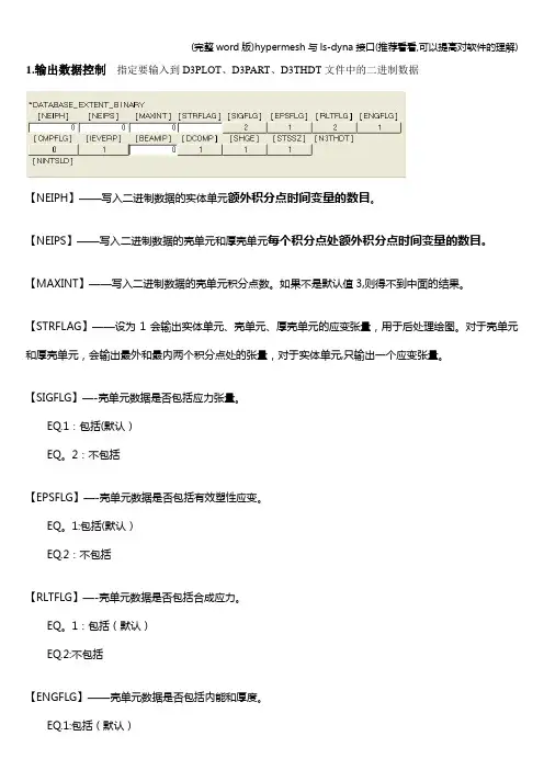
1.输出数据控制指定要输入到D3PLOT、D3PART、D3THDT文件中的二进制数据【NEIPH】——写入二进制数据的实体单元额外积分点时间变量的数目。
【NEIPS】——写入二进制数据的壳单元和厚壳单元每个积分点处额外积分点时间变量的数目。
【MAXINT】——写入二进制数据的壳单元积分点数。
如果不是默认值3,则得不到中面的结果。
【STRFLAG】——设为1会输出实体单元、壳单元、厚壳单元的应变张量,用于后处理绘图。
对于壳单元和厚壳单元,会输出最外和最内两个积分点处的张量,对于实体单元,只输出一个应变张量。
【SIGFLG】—-壳单元数据是否包括应力张量。
EQ.1:包括(默认)EQ。
2:不包括【EPSFLG】—-壳单元数据是否包括有效塑性应变。
EQ。
1:包括(默认)EQ.2:不包括【RLTFLG】—-壳单元数据是否包括合成应力。
EQ。
1:包括(默认)EQ.2:不包括【ENGFLG】——壳单元数据是否包括内能和厚度。
EQ.1:包括(默认)EQ。
2:不包括【CMPFLG】——实体单元、壳单元和厚壳单元各项异性材料应力应变输出时的局部材料坐标系。
EQ.0:全局坐标EQ。
1:局部坐标【IEVERP】--限制数据在1000state之内.EQ。
0:每个图形文件可以有不止1个stateEQ。
1:每个图形文件只能有1个state【BEAMIP】—-用于输出的梁单元的积分点数。
【DCOMP】——数据压缩以去除刚体数据。
EQ。
1:关闭(默认).没有刚体数据压缩。
EQ.2:开启。
激活刚体数据压缩。
EQ。
3:关闭.没有刚体数据压缩,但节点的速度和加速度被去除.EQ。
4:开启。
激活刚体数据压缩,同时节点的速度和加速度被去除。
【SHGE】-—输出壳单元沙漏能密度。
EQ。
1:关闭(默认).不输出沙漏能。
EQ。
2:开启。
输出沙漏能。
【STSSZ】——输出壳单元时间步、质量和增加的质量。
EQ。
1:关闭。
(默认)EQ.2:只输出时间步长。
基于LS-DYNA的电磁冲击器阀芯能量传递效率研究白威;王立华【摘要】阐述了电磁冲击器冲击时的能量转换过程,对电磁冲击器阀芯构建了有限元模型,并利用LS-DYNA软件对其冲击过程中阀芯的能量传递效率进行了研究,得出合理的结论,为以后冲击机械的设计开发和优化设计提供了可靠的依据.%This paper described the electromagnetic percussion and the energy conversion process, the impact of the electromagnetic valve device constructed finite element model. Using LS-DYNA software to its impact on the process efficiency of energy transfer spool, carried aut research and drew reasonable conclusions. The impact of the design for future development and optimization of mechanical design provided the reliable basis.【期刊名称】《新技术新工艺》【年(卷),期】2011(000)001【总页数】3页(P29-31)【关键词】电磁冲击器;能量转换;有限元;能量传递效率【作者】白威;王立华【作者单位】昆明理工大学,机电工程学院,河南,昆明,650093;昆明理工大学,机电工程学院,河南,昆明,650093【正文语种】中文【中图分类】TB52.3电磁冲击器是一种利用电磁力带动阀芯产生冲击的冲击机械,可以用于旧城改造、混凝土构件的拆毁、公路路基建设和钢厂炉渣拆卸等方面[1]。
在冲击过程中能量传递效率的大小是衡量冲击机械性能好坏的重要指标。
lsdyna 失效准则摘要:1.lsdyna 失效准则简介2.lsdyna 失效准则的分类3.lsdyna 失效准则的应用领域4.我国在失效准则研究方面的进展5.未来研究方向与挑战正文:lsdyna 失效准则是一种广泛应用于结构动力学分析的失效理论。
失效准则的制定旨在保证结构在各种工况下的安全性能。
本文将对lsdyna 失效准则进行简要介绍,并分析其在不同领域的应用及我国在该领域的研究进展。
1.lsdyna 失效准则简介lsdyna 失效准则起源于美国,是一种基于能量的失效理论。
它通过计算结构的能量变化,判断结构是否失效。
lsdyna 失效准则具有较高的计算精度和较强的适应性,能满足多种工况下的失效分析需求。
2.lsdyna 失效准则的分类lsdyna 失效准则主要分为以下几类:(1) 基于能量的失效准则,如能量释放率法、能量平衡法等。
(2) 基于变分原理的失效准则,如最大势能原理、最小势能原理等。
(3) 基于强度的失效准则,如强度折减法、等效应力法等。
3.lsdyna 失效准则的应用领域lsdyna 失效准则在以下领域得到了广泛应用:(1) 航空航天:用于分析飞行器结构在复杂工况下的安全性能。
(2) 汽车工程:用于评估汽车零部件在碰撞过程中的失效风险。
(3) 土木工程:用于预测桥梁、高楼等结构在风、地震等自然灾害下的抗灾能力。
(4) 机械制造:用于分析机床、起重设备等在极限载荷下的可靠性。
4.我国在失效准则研究方面的进展近年来,我国在失效准则研究方面取得了显著进展。
我国学者在引进、消化、吸收国外先进失效准则的基础上,发展了具有自主知识产权的失效理论。
此外,我国还积极参与国际失效准则标准的制定,为国际失效准则研究做出了贡献。
5.未来研究方向与挑战面对未来,失效准则研究仍然面临诸多挑战。
一方面,随着工程结构的日益复杂,失效准则需要不断优化和完善,以适应各种新型结构的安全分析需求。
另一方面,失效准则研究与计算机科学、材料科学等领域的交叉融合将成为新的研究热点。
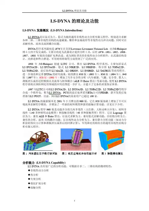
LS-DYNA 理论及功能LS-DYNA 的理论及功能LS-DYNA 发展概况 (LS-DYNA Introduction)LS-DYNA是以显式为主、隐式为辅的通用非线性动力分析有限元程序,特别适合求解 各种二维、三维非线性结构的高速碰撞、爆炸和金属成形等非线性动力冲击问题,同时可以 求解传热、流体及流固耦合问题。
DYNA 程序系列最初是 1976 年在美国 Lawrence Livermore National Lab. 由 J.O.Hallquist 博士主持开发完成的,主要目的是为武器设计提供分析工具,后经 1979、1981、1982、1986、 1987、1988 年版的功能扩充和改进,成为国际著名的非线性动力分析软件,在武器结构设 计、内弹道和终点弹道、军用材料研制等方面得到了广泛的应用。
1988 年 J.O.Hallquist 创建 LSTC 公司,推出 LS-DYNA 程序系列,主要包括显式 LS-DYNA2D、LS-DYNA3D、隐式 LS-NIKE2D、LS-NIKE3D、热分析 LS-TOPAZ2D、 LS-TOPAZ3D、前后处理 LS-MAZE、LS-ORION、LS-INGRID、LS-TAURUS 等商用程序, 进一步规范和完善 DYNA 的研究成果,陆续推出 930 版(1993 年)、936 版(1994 年)、940 版(1997 年),950 版(1998 年)增加了汽车安全性分析(汽车碰撞、气囊、安全带、假人)、 薄板冲压成形过程模拟以及流体与固体耦合(ALE 和 Euler 算法)等新功能,使得 LS-DYNA 程序系统在国防和民用领域的应用范围进一步扩大,并建立了完备的质量保证体系。
1997 年LSTC公司将LS-DYNA2D、LS-DYNA3D、LS-TOPAZ2D、LS-TOPAZ3D等程序 合成一个软件包,称为LS-DYNA,PC版的前后处理采用ETA公司的FEMB,新开发的后处 理器为LS-POST。
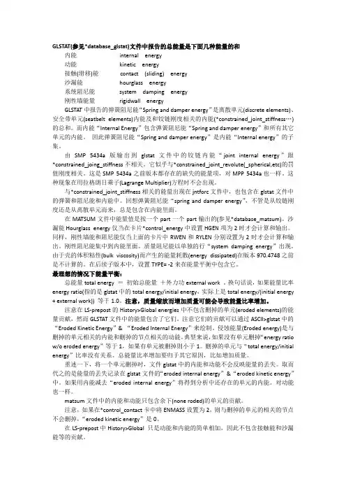
GLSTAT(参见*database_glstat)文件中报告的总能量是下面几种能量的和内能internal energy动能kinetic energy接触(滑移)能contact (sliding) energy沙漏能hourglass energy系统阻尼能system damping energy刚性墙能量rigidwall energyGLSTAT中报告的弹簧阻尼能“Spring and damper energy”是离散单元(discrete elements)、安全带单元(seatbelt elements)内能及和铰链刚度相关的内能(*constrained_joint_stiffness…)的总和。
而内能“Internal Energy”包含弹簧阻尼能“Spring and damper energy”和所有其它单元的内能。
因此弹簧阻尼能“Spring and damper energy”是内能“Internal energy”的子集。
由SMP 5434a版输出到glstat文件中的铰链内能“joint internal energy”跟*constrained_joing_stiffness不相关。
它似乎与*constrained_joint_revolute(_spherical,etc)的罚值刚度相关。
这是SMP 5434a之前版本都存在的缺失的能量项,对MPP 5434a也一样。
这种现象在用拉格朗日乘子(Lagrange Multiplier)方程时不会出现。
与*constrained_joint_stiffness相关的能量出现在jntforc文件中,也包含在glstat文件中的弹簧和阻尼能和内能中。
回想弹簧阻尼能“spring and damper energy”,不管是从铰链刚度还是从离散单元而来,总是包含在内能里面。
在MATSUM文件中能量值是按一个part一个part输出的(参见*database_matsum)。
第一章LS-DYNA简介1.1 LS-DYNA发展概况DYNA程序系列最初是1976年在美国Lawrence Livermore National Lab. 由J.O.Hallquist 博士主持开发完成的,主要目的是为武器设计提供分析工具,后经1979、1981、1982、1986、1987、1988年版的功能扩充和改进,成为国际著名的非线性动力分析软件,在武器结构设计、内弹道和终点弹道、军用材料研制等方面得到了广泛的应用。
1988年J.O.Hallquist创建LSTC公司,推出LS-DYNA程序系列,主要包括显式LS-DYNA2D、LS-DYNA3D、隐式LS-NIKE2D、LS-NIKE3D、热分析LS-TOPAZ2D、LS-TOPAZ3D、前后处理LS-MAZE、LS-ORION、LS-INGRID、LS-TAURUS等商用程序,进一步规范和完善DYNA的研究成果,陆续推出930版(1993年)、936版(1994年)、940版(1997年),增加了汽车安全性分析(汽车碰撞、气囊、安全带、假人)、薄板冲压成型过程模拟,以及流体与固体耦合(ALE和Euler算法)等新功能,使得LS-DYNA程序系统在国防和民用领域的应用范围进一步扩大,并建立了完备的质量保证体系。
1997年LSTC公司将LS-DYNA2D、LS-DYNA3D、LS-TOPAZ2D、LS-TOPAZ3D等程序合成一个软件包,称为LS-DYNA,PC版的前后处理采用ETA公司的FEMB,新开发的后处理器为LS-POST。
1996年LSTC与ANSYS公司合作推出ANSYS/LS-DYNA,大大增强了LS-DYNA的分析能力,用户可以充分利用ANSYS的前后处理和统一数据库的优点。
2001年5月推出960版,它在950版基础上增加了不可压缩流体求解程序模块,并增加了一些新的材料模型和新的接触计算功能,从2001年到2003年初LSTC公司不断完善960版的新功能,2003年3月正式发布970版。
LS-DYNA 程序采用动力松弛技术,可以进行动力分析前的预应力计算或者进行静力分析。
LS-DYNA3D 程序的算法基础: (1)控制方程1.动量方程:i i j j x f ..,i ρρσ=+ij σ为柯西应力 i f 为单位质量体积力 ..x 为加速度2.质量守恒:0ρρJ =ρ为当前质量密度 0ρ为初始质量密度 J 为体积变化率3.能量方程V )(VS E ij ij q p +-=。
ε………………………………………………………….(2.5)用于状态方程计算 和 总的能量平衡。
式中,V 为现时构形的体积;ij 。
ε为应变率张量;q 为体积粘性阻力 偏应力ij ij ij q p S σσ)(++= 压力q p kk --=σ31力分量的边界值就等于对应的面力分量,如下式表示))(t t n i j ij =σ在1S 面力边界上式中:j n ,j=1,2,3为现时构形边界1S 的外法线方向余弦;i t ,i=1,2,3为面力载荷b.位移边界条件(在位移边界问题中,物体在全部或部分边界u s 上的位移分量都是已知函数,即在边界上有:)()(s u u s = )()(s v v s = )()(s w w s =,其中s u )(、s v )(、s w )(是位移函数在边界上的值,)(s u 、)(s v 、)(s w 表示边界上的已知位移分量,例如对于完全固定边界0===w v u ,有0)(=s u ,0)(=s v ,0)(=s w ))(),(t K t X x i j i =在2S 位移边界上式中,)(t K i ,i=1,2,3是给定位移函数 c.滑动接触面间断处的跳跃条件单元内某一点的自然坐标表示成e x N t x }]{[)},,,({=ςηξ式中,单元内任意点在t 时刻的坐标矢量Tt x )},,,({ςηξ=[1x 2x 3x ]单元节点坐标矢量],,,...,,[}{838281131211x x x x x x x eT =插值矩阵2438181810 (0000) (0000)...00)],,([⨯⎥⎥⎥⎦⎤⎢⎢⎢⎣⎡=φφφφφφςηξNLS-DYNA3D 程序将单元质量矩阵⎰=mV TNdV N m ρ的同一行矩阵元素都合并到对角元素项,形成集中质量矩阵。
一、【子程序】vumat有沙漏问题么?沙漏问题和VUMAT无关,跟你选择的单元有关系,如果你采用减缩积分单元,则会存在沙漏。
有限元的一个核心就是单元模型,其思想是采用单元近似连续体,单元内采用形函数进行插值。
采用全积分的话,可以精确地积出刚度矩阵,但是采用全积分会导致有限元过刚,例如体积锁死和剪切锁死等,因此很多力学及提出了各种各样的单元模型来解决这些问题。
现在用的较多的低阶单元就是一点积分,一点积分的单元由于积分点过少而存在零能模式(沙漏),即在某些变形模式下会出现零应变,这个可以从形函数的公式中推导出来。
所以,沙漏模式是否存在取决你选用的单元,但是你采用ABAQUS的默认设置基本上就可以解决这个问题。
不知道我有没有说清楚二、【基础理论】【概念】剪切锁死、体积锁死、沙漏、零能模式1.剪切锁死(shear locking)简单地说就是在理论上没有剪切变形的单元中发生了剪切变形。
该剪切变形也常称伴生剪切(parasitic shear)。
发生的条件:1.一阶、全积分单元;2.受纯弯状态;产生的结果:使得弯曲变形偏小,即弯曲刚度太刚。
解决方法:1.采用减缩积分;2.细化网格;3.非协调单元;4.假定剪切应变法;2.体积锁死(volumetric locking)简单地说就是应该有单元的体积变化的时候体积却没发生变化。
该原因是受到了伪围压应力(Spurious pressure stresses )。
发生的条件:1.全积分单元;2.材性几乎不可压缩;二阶单元:对于弹塑性材料(塑性部分几乎属于不可压缩),二阶全积分四边形和六面体单元在塑性应变和弹性应变在一个数量级时会发生体积锁死。
二次减缩积分单元发生大应变时体积锁死也伴随出现。
但值得注意的是,一阶全积分单元当采用选择性减缩积分(selectively reduced integration)时可以避免出现体积锁死。
产生的结果:使得体积不变,即体积模量太大,刚度太刚。
Total energyTotal energy reported in GLSTAT (see *DATABASE_GLSTAT ) is the sum of∙internal energy∙kinetic energy∙contact (sliding) energy∙hourglass energy∙system damping energy∙rigidwall energySpring and damper energy reported in the glstat file is the sum of internal energy of discrete elements, seatbelt elements, and energy associated with joint stiffnesses (*CONSTRAINED_JOINT_STIFFNESS....). Internal Energy includes Spring and damper energy as well as internal energy of all other element types. Thus Spring and damper energy is a subset of Internal energy.The joint internal energy written to glstat by SMP 5434a is independent of the *CONSTRAINED_JOINT_STIFFNESS. It would appear to be associated with the penalty stiffness of *CONSTRAINED_JOINT_REVOLUTE (_spherical, etc). This was a missing energy term prior to SMP rev. 5434a. It is still a missing energy term in MPP rev. 5434a. If Jason hasn't already added this energy term to MPP in a more recent revision than 5434a, he probably should do so.The energy associated with *CONSTRAINED_JOINT_STIFFNESS appears in the jntforc file and is included in glstat in spring and damper energy and internal energy. Recall that spring and damper energy, whether from joint stiffness or from discrete elements, is always included in internal energy.Energy values are written on a part-by-part basis in MATSUM see*DATABASE_MATSUM).Hourglass energy is computed and written only if HGEN is set to 2 in *CONTROL_ENERGY. Likewise, rigidwall energy and system damping energy are computed and written only if RWEN and RYLEN, respectively, are set to 2.Stiffness damping energy is lumped into internal energy. Mass damping energy appears as a separate line item system damping energy.Energy dissipated due to shell bulk viscosity was not calculated prior to revision 4748 of v. 970. It is subsequently an option to include this energy in the energy balance.The energy balance is perfect if total energy = initial total energy + external work, or in other words if the energy ratio (referred to in GLSTAT as total energy / initial energy although it actually is total energy / (initial energy + external work)) is equal to 1.0.The History > Global energies do not include the contributions of eroded elements whereas the GLSTAT energies do include those contributions. Note that these eroded contributions can be plotted as Eroded Kinetic Energy and Eroded Internal Energy via ASCII > GLSTAT.Eroded energy is the energy associated with deleted elements (internal energy) and deleted nodes (kinetic energy). Typically, the energy ratio w/o eroded energy would be equal to 1 if no elements have been deleted or less than one if elements have been deleted. The deleted elements should have no bearing on the total energy / initial energy ratio. Overall energy ratio growth would be attributable to some other event, e.g., added mass.An example is attached. Note that if ENMASS in *CONTROL_CONTACT is set to 2, the nodes associated with the deleted elements are not deleted and the eroded kinetic energy is zero.The total energy via History > Global is simply the sum of KE and internal energies and thus doesn't include such contributions as contact energy or hourglass energy.Negative internal energy in shells:To combat this spurious effect, - turn off shell thinning (ISTUPD) - invoke bulk viscosity for shells (set TYPE = -2 in *CONTROL_BULK_VISCOSITY ) - use *DAMPING_PART_STIFFNESS for parts exhibiting neg. IE in matsum Try a small value first, e.g., .01. If RYLEN=2 in *CONROL_ENERGY, then the energy due to stiffness damping is calculated and included in internal energy. (See negative_internal_energy_in_shells for a case study)Positive contact energy:When friction is included in a contact definition, positive contact is to be expected. Friction SHOULD result in positive contact energy. In the absence of friction, you would hope to see a small net contact energy (net = sum of slave side energy and master side energy). Small is a matter ofjudgement -- 10% of peak internal energy might be considered acceptable for contact energy in the absence of contact friction.Negative contact energy:Abrupt increases in negative contact energy may be caused by undetected initial penetrations. Care in defining the initial geometry so that shell offsets are properly taken into account is usually the most effective step to reducing negative contact energy. Refer to sections 23.8.3 and 23.8.4 in the LS-DYNA Theory Manual (May 1998) for more information on contact energy.Negative contact energy sometimes is generated when parts slide relative to each other. This has nothing to do with friction. I'm speaking of negative energy from normal contact forces and normal penetrations. When a penetrated node slides from its original master segment to an adjacent though unconnected master segment and a penetration is immediately detected, negative contact energy is the result.If internal energy mirrors negative contact energy, i.e., the slope of internal energy curve in glstat is equal and opposite that of the negative contact energy curve, it;s possible that the problem is very localized with low impact on the overall validity of the solution. You may be able to isolate the local problem area(s) by fringing internal energy of your shell parts (Fcomp > Misc > internal energy in LS-POST). Hot spots in internal energy usually indicate where negative contact energy is focused.If you have more than one contact defined, the sleout file(*DATABASE_SLEOUT) will report contact energies for each contact and so the focus of the negative contact energy investigation can be narrowed.Some general suggestions for combating negative contact energy are as follows:∙Eliminate initial penetrations (look for Warning in messag file).∙Check for and eliminate redundant contact conditions. Y ou should NOT have more than one contact definition treating contact between the same two parts or surfaces.∙Reduce the time step scale factor.∙Set contact controls back to default except set SOFT=1 and IGNORE=1 (Optional CardC).∙For contact of sharp-edged surfaces, set SOFT=2 (applicable for segment-to-segment contact only). Furthermore, in v. 970, setting SBOPT (formerly EDGE) to 4 isrecommended for SOFT=2 contact where relative sliding between parts occurs. Forimproved edge-to-edge SOFT=2 contact behavior, set DEPTH to 5. Please note thatSOFT=2 contact carries some additional expense, particularly using nondefault values ofSBOPT or DEPTH, and so should be used only where other contact options (SOFT=0 orSOFT=1) are inadequate.The specifics of your model may dictate that some other approach be used. jpd last revised 5/14/2003。
在判断一个模型的计算结果是否合理的时候,首先应该检查能量是否合理。
比如,是否有负的接触能量(Sliding energy)。
建模的时候,只要设定了接触(*CONTACT),就会在相应的两个接触面(Master side & Slave side)上产生能量,通过设定*DATABASE_SLEOUT可以输出各个设定的接触面的能量。
如果一个接触里,总能量是负值,就说明单元之间有互相穿入。
如果设定了*DATABASE_GLSTAT,可以输出模型的总能量,包括总的接触面能量。
只检查总的接触能量,可能会掩盖一些问题,比如设定了n个接触,其中第m个接触有很大的负能量,但是在计算总能量的时候,如果另外n-1个接触的正能量,抵消了m的负能量,总接触能量会显得比较合理。
个人经验,如果接触能量为负(总接触能,或某个接触上产生的最大负接触能),其绝对值以不能超过总能量的1/20为好。
LSDYNA中的能量平衡time........................... 4.99735E-03time step...................... 4.45000E-06kinetic energy................. 3.80904E+09internal energy................ 5.15581E+09spring and damper energy....... 1.00000E-20hourglass energy .............. 1.34343E+08system damping energy.......... 0.00000E+00sliding interface energy....... 1.72983E+07external work.................. 4.54865E+09eroded kinetic energy.......... 0.00000E+00eroded internal energy......... 0.00000E+00total energy................... 9.11649E+09total energy / initial energy.. 1.09716E+00energy ratio w/o eroded energy. 1.09716E+00global x velocity.............. -6.63878E+01global y velocity.............. 3.44465E+02global z velocity.............. -1.86129E+04time per zone cycle.(nanosec).. 11286GLSTAT(参见*database_glstat)文件中报告的总能量是下面几种能量的和:内能 internal energy动能 kinetic energy接触(滑移)能 contact(sliding) energy沙漏能 houglass energy系统阻尼能 system damping energy刚性墙能量 rigidwall energyGLSTAT中报告的弹簧阻尼能”Spring and damper energy”是离散单元(discrete elements)、安全带单元(seatbelt elements)内能及和铰链刚度相关的内能(*constrained_joint_stiffness…)之和。
而内能”Internal Energy”包含弹簧阻尼能”Spring and damper energy”和所有其它单元的内能。
因此弹簧阻尼能”Spring and damper energy”是内能”Internal energy”的子集。
由SMP5434a版输出到glstat文件中的铰链内能”joint internal energy”跟*constrained_joing_stiffness不相关。
它似乎与*constrained_joint_revolute(_spherical,etc)的罚值刚度相关连。
这是SMP 5434a之前版本都存在的缺失的能量项,对MPP 5434a也一样。
这种现象在用拉格朗日乘子(Lagrange Multiplier)方程时不会出现。
与*constrained_joint_stiffness相关的能量出现在jntforc文件中,也包含在glstat文件中的弹簧和阻尼能和内能中。
回想弹簧阻尼能”spring and damper energy”,不管是从铰链刚度还是从离散单元而来,总是包含在内能里面。
在MATSUM文件中能量值是按一个part一个part的输出的(参见*database_matsum)。
沙漏能Hourglass energy仅当在卡片*control_energy中设置HGEN项为2时才计算和输出。
同样,刚性墙能和阻尼能仅当上面的卡片中RWEN和RYLEN分别设置为2时才会计算和输出。
刚性阻尼能集中到内能里面。
质量阻尼能以单独的行”system damping energy”出现。
由于壳的体积粘性(bulk viscosity)而产生的能量耗散(energy dissipated)在版本970.4748之前是不计算的。
在后续子版本中,设置TYPE=-2来在能量平衡中包含它。
最理想的情况下能量平衡:总能量total energy =初始总能量+外力功external work。
换句话说,如果能量比率energy ratio(指的是glstat中的total energy/initial energy,实际上是total energy/(initial energy + external work)) 等于1.0。
注意,质量缩放而增加质量可能会导致能量比率增加。
注意在LSprepost的History>Global energies中不包含删掉的单元(eroded elements)的能量贡献,然而GLSTAT文件中的能量包含了它们。
注意它们的贡献可以通过ASCII>glstat中的”Eroded Kinetic Energy”& “Eroded Internal Energy”来绘制。
侵蚀能量(Eroded energy)是与删掉的单元相关的内能和删掉的节点相关的动能。
典型来说,如果没有单元删掉”energy ratio w/o eroded energy”等于1,如果有单元被删掉则小于1。
删掉的单元与”total energy/initial energy”比率没有关系。
总能量比率增加要归于其它原因,比如增加质量。
重述一下,将一个单元删掉时,文件glstat中的内能和动能不会反映能量的丢失。
取而代之的是能量的丢失记录在glstat文件的”eroded internal energy” & “eroded kinetic energy”中。
如果用内能减去”eroded internal energy”将得到分析中还存在的单元的内能。
对动能也一样。
matsum文件中的内能和动能只包含余下(noneroded)的单元的贡献。
注意,如果在*control_contact卡中将ENMASS设置为2,则与删掉的单元的相关的节点不会删掉,”eroded kinetic energy”是0。
在LSprepost中History>Global 只是动能和内能的简单相加,因此不包含接触能和沙漏能等的贡献。
----------壳的负内能:为了克服这种不真实的效应--关掉考虑壳的减薄(ISTUPD in *control_shell)--调用壳的体积粘性(set TYPE=-2 在*control_bulk_viscosity卡中)--对在matsum文件中显示为负的内能的parts使用*damping_part_stiffness;先试着用一个小的值,比如0.01如果在*control_energy中设置RYLEN=2,因为刚性阻尼而能会计算且包含在内能中。
----------正的接触能:当在接触定义中考虑了摩擦时将得到正的接触能。
摩擦将导致正的接触能。
如果没有设置接触阻尼和接触摩擦系数,你将会看到净接触能为零或者一个很小的值(净接触能=从边和主边能量和)。
所说的小是根据判断-在没有接触摩擦系数时,接触能为峰值内能的10%内可以被认为是可接受的。
----------负的接触能:突然增加的负接触能可能是由于未检测到的初始穿透造成的。
在定义初始几何时考虑壳的厚度偏置通常是最有效的减小负接触能的步骤。
查阅LS-DYNA理论手册的23.8.3&23.8.4节可得到更多接触能的信息。
负接触能有时候因为parts之间的相对滑动而产生。
这跟摩擦没有关系,这里说的负接触能从法向接触力和法向穿透产生。
当一个穿透的节点从它原来的主面滑动到临近的没有连接的主面时,如果穿透突然检测到,则产生负的接触能。
如果内能为负接触能的镜像,例如glstat文件中内能曲线梯度与负接触能曲线梯度值相等,问题可能是非常局部化的,对整体求解正确性冲击较小。
你可以在LS-prepost中分离出有问题的区域,通绘制壳单元部件内能云图(Fcomp > Misc > Internal energy)。
实际上,显示的是内能密度,比如内能/体积。
内能密度云图中的热点通常表示着负的接触能集中于那里。
如果有多于一个的接触定义,sleout文件(*database_sleout)将报告每一个接触对的接触能量,因此缩小了研究负接触能集中处的范围。
克服负接触能的一般的建议如下:-消除初始穿透(initial penetration)。
(在message文件中查找”warning”)-检查和排除冗余的接触条件。
不应该在相同的两个parts之间定义多于一个的接触。
-减小时间步缩放系数-设置接触控制参数到缺省值,SOFT=1 & IGNORE=1除外(接触定义选项卡C)-对带有尖的边的接触面,设置SOFT=2(仅用于segment-to-segment接触)。
而且,在版本970中推荐设置SBOPT(之前的EDGE)为4对于部件之间有相对滑移的SOFT=2的接触。
为了改进edge-to-edge SOFT=2接触行为,设置DEPTH=5。
请注意SOFT=2接触增加了额外的计算开消,尤其是当SBOPT或者DEPTH不是缺省值时,因此应该仅在其它接触选项(SOFT=0或者SOFT=1)不能解决问题时。
English version:Total energy reported in GLSTAT (see *database_glstat) is the sum of …internal energykinetic energycontact (sliding) energyhourglass energysystem damping energyrigidwall energy“Spring and damper energy” reported in the glstat file is the sum of internal energy of discrete elements, seatbelt elements, and energy associated with joint stiffnesses (*constrained_joint_stiffness….). “Internal Energy” includes “Spring and damper energy” as well as internal energy of all other element types. Thus “Spring and damper energy” is a subset of “Internal energy”.The “joint internal energy” written to glstat by SMP 5434a is independent of the constrained_joint_stiffness. It would appear to be associated with the penalty stiffnessof *constrained_joint_revolute (_spherical, etc). This was a missing energy term prior to SMP rev. 5434a. It is still a missing energy term in MPP rev. 5434a. It does NOT appear when a Lagrange Multiplier formulation is used.The energy associated with *constrained_joint_stiffness appears in the jntforc file and is included in glstat in “spring and damper energy” and “internal energy”. Recall that “spring and damper energy”, whether from joint stiffness or from discrete elements,is always included in “internal energy”.Energy values are written on a part-by-part basis in MATSUM (see *database_matsum). Hourglass energy is computed and written only if HGEN is set to 2 in *control_energy. Likewise, rigidwall energy and damping energyare computed and written only if RWEN and RYLEN, respectively, are set to 2. Stiffness damping energy is lumped into internal energy.Mass damping energy appears as a separate line item “system damping energy”.Energy dissipated due to shell bulk viscosity was not calculated prior to revision 4748 of v. 970. In subsequent revisions, set TYPE=-2 to iclude this energy in the energy balance.The energy balance is perfect if total energy = initial total energy + external work, or in other words if the energy ratio (referred to in glstat as “total energy / initial energy”although it actually is total energy / (initial energy + external work)) is equal to 1.0.Note that added mass may cause the energy ratio to rise. (See~/test/erode/taylor.mat3.noerode.mscale.k)The History > Global energies do not include the contributions of eroded elements whereasthe GLSTAT energies do include those contributions.Note that these eroded contributions can be plotted as “Eroded Kinetic Energy”and “Eroded Internal Energy” via ASCII > glstat. Eroded energy is the energy associated with deleted elements (internal energy) and deleted nodes (kinetic energy). Typically, the “energy ratio w/o eroded energy” would be equal to 1 if no elements have been deletedor less than one if elements have been deleted. The deleted elements should have no bearing on the “total energy / initial energy” ratio. Overall energy ratio growth would be attributable to some other event, e.g., added mass.Restated, when an element erodes, the internal energy and kinetic energy in glstat do not reflect the energy loss. Instead the energy losses are recorded as “eroded internal energy” and “eroded kinetic energy” in glstat. If you subtract “eroded internal energy” from “internal energy”, you have the internal energy of elements which remainin the simulation. Likewise for kinetic energy. The matsum file’s internal energy and kinetic energy include only contributions from the remaining (noneroded) elements.An example is attached. Note that if ENMASS in *control_contact is set to 2, the nodes associated with the deleted elements are not deleted and the “eroded kinetic energy” is zero. (See ~/test/m3ball2plate.15.k)The total energy via History > Global is simply the sum of KE and internal energies and thus doesn’t include such contributions as contact energy or hourglass energy.Negative internal energy in shells:To combat this spurious effect,- turn off shell thinning (ISTUPD)- invoke bulk viscosity for shells (set TYPE = -2 in *control_bulk_viscosity)- use *damping_part_stiffness for parts exhibiting neg. IE in matsumTry a small value first, e.g., .01.If RYLEN=2 in *control_energy, then the energy due to stiffness damping is calculated and included in internal energy.(See negative_internal_energy_in_shells for a case study)Positive contact energy:When friction is included in a contact definition, positive contact is to be expected. Friction SHOULD result in positive contact energy.In the absence of contact damping and contact friction,one would hope to see zero (or very small) net contact energy (net = sum of slave side energy and master side energy). “Small” is a matter of judgement — 10% of peak internal energy might be considered acceptable for contact energy in the absence of contact friction. (~/test/shl2sol/sphere_to_plate.examine_contact_damping_energy.k appears to illustrate that contact damping (VDC = 0, 30, 90) produces positive sliding (or contact) energy)Negative contact energy:Refer to p. 3.14, 3.15 of “Crashworthiness Engineering Course Notes” by Paul Du Bois. Contact jane@ to purchase these notes.Abrupt increases in negative contact energy may be caused by undetected initial penetrations. Care in defining the initial geometry so that shell offsets are properly taken into account is usually the most effective step to reducing negative contact energy. Refer to sections 23.8.3 and 23.8.4 in the LS-DYNA Theory Manual (May 1998) for more information on contact energy.Negative contact energy sometimes is generated when parts slide relative to each other. This has nothing to do with friction — I’m speaking of negative energy from normal contact forces and normal penetrations. When a penetrated node slides from its original master segment to an adjacent though unconnected master segment and a penetration is immediately detected, negative contact energy is the result.If internal energy mirrors negative contact energy, i.e., the slope of internal energy curve in glstat is equal and opposite that of the negative contact energy curve, it could be that the problem is very localized with low impact on the overall validity of the solution. You may be able to isolate the local problem area(s) by fringing internal energy of your shell parts (Fcomp > Misc >internal energy in LS-Prepost). Actually, internal energy density is displayed, i.e., internal energy/volume. Hot spots in internal energy density usually indicate where negative contact energy is focused.If you have more than one contact defined, the sleout file (*database_sleout) will report contact energies for each contact and so the focus of the negative contact energy investigation can be narrowed.Some general suggestions for combating negative contact energy are as follows:- Eliminate initial penetrations (look for “Warning” in messag file).- Check for and eliminate redundant contact conditions. You should NOT have more than one contact definition treating contact between the same two parts or surfaces.- Reduce the time step scale factor.- Set contact controls back to default except set SOFT=1 and IGNORE=1 (Optional Card C). - For contact of sharp-edged surfaces, set SOFT=2 (applicable for segment-to-segment contact only). Furthermore, in v. 970, setting SBOPT (formerly EDGE) to 4 is recommended for SOFT=2 contact where relative sliding between parts occurs. For improved edge-to-edge SOFT=2 contact behavior, set DEPTH to 5. Please note that SOFT=2 contact carries some additional expense, particularly using nondefault values of SBOPT or DEPTH, and so should be used only where other contact options (SOFT=0 or SOFT=1) are inadequate.。