计量经济学导论第五版第一章上机作业.(精选)
- 格式:doc
- 大小:200.50 KB
- 文档页数:13
APPENDIX ASOLUTIONS TO PROBLEMSA.1 (i) $566.(ii) The two middle numbers are 480 and 530; when these are averaged, we obtain 505, or $505.(iii) 5.66 and 5.05, respectively.(iv) The average increases to $586 while the median is unchanged ($505).A.3 If price = 15 and income = 200, quantity = 120 – 9.8(15) + .03(200) = –21, which is nonsense. This shows that linear demand functions generally cannot describe demand over a wide range of prices and income.A.5 The majority shareholder is referring to the percentage point increase in the stock return, while the CEO is referring to the change relative to the initial return of 15%. To be precise, the shareholder should specifically refer to a 3 percentage point increase.$45,935.80.≈ $40,134.84. When exper = 5, salary = exp[10.6 + .027(5)] ≈A.7 (i) When exper = 0, log(salary) = 10.6; therefore, salary = exp(10.6) (ii) The approximate proportionate increase is .027(5) = .135, so the approximate percentage change is 13.5%.14.5%, so the exact percentage increase is about one percentage point higher.≈(iii) 100[(45,935.80 – 40,134.84)/40,134.84)A.9 (i) The relationship between yield and fertilizer is graphed below. (ii) Compared with a linear function, the functionyieldhas a diminishing effect, and the slope approaches zero as fertilizer gets large. The initial pound of fertilizer has the largest effect, and each additional pound has an effect smaller than the previous pound.APPENDIX BSOLUTIONS TO PROBLEMSB.1 Before the student takes the SAT exam, we do not know – nor can we predict with certainty – what the score will be. The actual score depends on numerous factors, many of which we cannot even list, let alone know ahead of time. (The student’s innate ability, how the student feels on exam day, and which particular questions were asked, are just a few.) The eventual SAT score clearly satisfies the requirements of a random variable.B.3 (i) Let Yit be the binary variable equal to one if fund i outperforms the market in year t. By assumption, P(Yit = 1) = .5 (a 50-50 chance of outperforming the market for each fund in each year). Now, for any fund, we are also assuming that performance relative to the market isP(Yi2 = 1) P(Yi,10 = 1) = (.5)10 = 1/1024 (which is slightly less than .001). In fact, if we define a binary random variable Yi such that Yi = 1 if and only if fund i outperformed the market in all 10 years, then P(Yi = 1) =1/1024.⋅independent across years. But then the probability that fund i outperforms the market in all 10 years, P(Yi1 = 1,Yi2 = 1, , Yi,10 = 1), is just the product of the probabilities: P(Yi1 = 1).983. This means, if performance relative to the market is random and independent across funds, it is almost certain that at least one fund will outperform the market in all 10 years.≈P(Y4,170 = 0) = 1 –(1023/1024)4170 ⋅⋅⋅ P(Y2 = 0)⋅= 1/1024. We want to compute P(X ≥ 1) =1 – P(X = 0) = 1 –P(Y1 = 0, Y2 = 0, …, Y4,170 = 0) = 1 – P(Y1 = 0)θ)distribution with n = 4,170 and θ(ii) Let X denote the number of funds out of 4,170 that outperform the market in all 10 years. Then X = Y1 + Y2 + + Y4,170. If we assume that performance relative to the market is independent across funds, then X has the Binomial (n,(iii) Using the Stata command Binomial(4170,5,1/1024), the answer is about .385. So there is a nontrivial chance that at least five funds will outperform the market in all 10 years..931.≈ 1) = 1 – P(X = 0) = 1 – (.8)12 ≥B.5 (i) As stated in the hint, if X is the number of jurors convinced of Simpson’s innocence, then X ~ Binomial(12,.20). We want P(X(ii) Above, we computed P(X = 0) as about .069. We need P(X = 1), which we obtain from1 – (.069 + .206) = .725, so there is almost a three in four chance that the jury had at least two members convinced of Simpson’s innocence prior to the trial.≈ 2) ≥ .206. Therefore, P(X ≈ (.2)(.8)11 ⋅ = .2, and x = 1:P(X = 1) = 12θ(B.14) with n = 12,B.7 In eight attempts the expected number of free throws is 8(.74) = 5.92, or about six free throws.X, and so the expected value of Y is 1,000 times the expected value of X, and the standard deviation of Y is 1,000 times the standard deviation of X. Therefore, the expected value and standard deviation of salary, measured in dollars, are $52,300 and $14,600, respectively.⋅B.9 If Y issalary in dollars then Y = 1000。
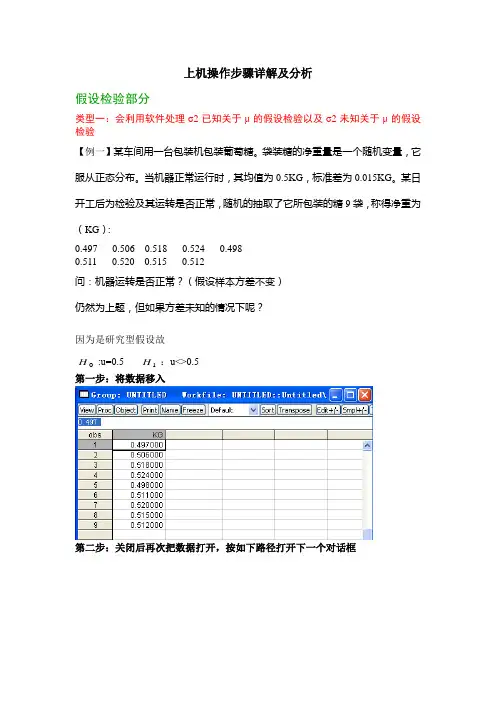
上机操作步骤详解及分析假设检验部分类型一:会利用软件处理σ2已知关于μ的假设检验以及σ2未知关于μ的假设检验【例一】某车间用一台包装机包装葡萄糖。
袋装糖的净重量是一个随机变量,它服从正态分布。
当机器正常运行时,其均值为0.5KG ,标准差为0.015KG 。
某日开工后为检验及其运转是否正常,随机的抽取了它所包装的糖9袋,称得净重为(KG ):0.497 0.506 0.518 0.524 0.498 0.511 0.520 0.515 0.512问:机器运转是否正常?(假设样本方差不变) 仍然为上题,但如果方差未知的情况下呢?因为是研究型假设故0H :u=0.5 1H :u<>0.5第一步:将数据移入第二步:关闭后再次把数据打开,按如下路径打开下一个对话框第三步:根据已知的均值和标准差输入下列对话框(注意:是标准差,如果题目告诉的是方差,则还要进一步转化成为标准差)第四步:点击OK后,得到如下结果,并分析该题的方差已知,故看Z-statistic的P值,因为0.0248<a/2=0.025,故拒绝原假设,结论为:在5%的显著性水平下,该机器运转不正常若该题的方差未知,则看t-statistic的P值,结论依然是:在5%的显著性水平下,该机器运转不正常类型二:会利用软件处理来自两个正态总体均值的假设检验:等方差和异方差【例2】用两种方法(A、B)测定冰从-0.72摄氏度变为0摄氏度的比热。
测得下列数据:两个样本独立且来自与方差相等的两个正态总体方法A 79.98 80.04 80.02 80.04 80.03 80.0380.04 79.97 80.05 80.03 80.02 80.00 80.02方法B 80.02 79.94 79.98 79.97 79.97 80.03 79.9579.971、两种方法是否具有显著性差异2、A方法是否比B方法测得的比热要大?解析:该题属于双样本的等方差检验,故在EXCEL背景下操作第一小问:第一步:移入数据,将原本的两行数据,分别调整为一行第二步:EXCEL的调试,“工具”——“加载宏”后选择如下选项:第三步:点击“工具”——“数据分析”——“t检验-双样本等方差检验”第四步:输入相应的数据第五步:分析相应结果解析:第一小问只需判断是否有显著性差异,也就是说只需要判断A U 与B U 是否相等,属于双侧检验,在统一用P(T<=t) 单尾分析的时候,与的是a/2比较0H :AU-B U =0 1H :A U -B U <>0如上图结果所示,P(T<=t) 单尾=0.001276<a/2=0.025,所以拒绝原假设,也就是说在5%的显著性水平下,方法A 和方法B 具有显著性差异第二小问:解析:第二小问不同于第一小问,判断的是A 与B 的大小,是研究型假设检验, 将认为研究结果是无效的说法或理论作为原假设H00H :AU<=B U 1H :A U >B U因为是单侧检验,故与a 相比,因为P(T<=t) 单尾=0.001276<a=0.05,所以拒绝原假设,结论是在5%的显著性水平下,A 方法测得的比热比B 方法的大【例3】下表给出两位文学家马克吐温的8篇小品文以及斯诺特格拉斯的10篇小品文中由3个字母组成的单字的比例 马克吐温0.225 0.262 0.217 0.240 0.2300.229 0.235 0.217 斯诺特格拉斯0.209 0.205 0.196 0.210 0.202 0.207 0.224 0.223 0.2200.201两组数据均来自正态总体,且方差相等。
计量经济学导论第一次作业(第四组)伍德里奇
计量经济学导论第一次作业
(第4组)
第一题:设计一假想的理想化随机对照试验来研究系上安全带对高速公路上交通死亡事故产生的影响。
试提出实施这个实验可能遇到的障碍。
两组试验:随机抽取两组汽车租赁公司,一组司机每天驾驶必须系安全带,一组司机未系安全带。
进行一个月的有效数据跟踪监测。
统计两组事故发生率。
障碍:1、道德约束,不可能让所有司机违反交通规则。
2、司机会有性别、驾驶员驾驶的驾驶年龄不同等其他因素的影响。
第二题:
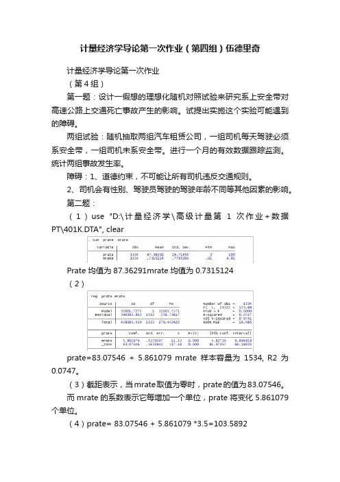
(1)use "D:\计量经济学\高级计量第1次作业+数据PT\401K.DTA", clear
Prate 均值为87.36291mrate均值为0.7315124
(2)
prate=83.07546 + 5.861079 mrate样本容量为1534, R2为0.0747。
(3)截距表示,当mrate取值为零时,prate的值为83.07546。
而mrate的系数表示它每增加一个单位,prate将变化5.861079个单位。
(4)prate= 83.07546 + 5.861079 *3.5=103.5892
预测值为103.5892不合适,最高为100%,还有就是一般取值应该在均值附近,3.5这个值太靠右。
(5)方程拟合程度0.0747调整后0.0741具体prate的变异可能并不都是由mrate造成,还需要进一步进行检验及考虑其他变量。
对于样本数量,养老金是一个大群体,人口占国家数量很大。
该数量太少。

APPENDIX ASOLUTIONS TO PROBLEMSA.1 (i) $566.(ii) The two middle numbers are 480 and 530; when these are averaged, we obtain 505, or $505.(iii) 5.66 and 5.05, respectively.(iv) The average increases to $586 while the median is unchanged ($505).A.3 If price = 15 and income = 200, quantity = 120 – 9.8(15) + .03(200) = –21, which is nonsense. This shows that linear demand functions generally cannot describe demand over a wide range of prices and income.A.5 The majority shareholder is referring to the percentage point increase in the stock return, while the CEO is referring to the change relative to the initial return of 15%. To be precise, the shareholder should specifically refer to a 3 percentage point increase.$45,935.80.≈ $40,134.84. When exper = 5, salary = exp[10.6 + .027(5)] ≈A.7 (i) When exper = 0, log(salary) = 10.6; therefore, salary = exp(10.6) (ii) The approximate proportionate increase is .027(5) = .135, so the approximate percentage change is 13.5%.14.5%, so the exact percentage increase is about one percentage point higher.≈(iii) 100[(45,935.80 – 40,134.84)/40,134.84)A.9 (i) The relationship between yield and fertilizer is graphed below. (ii) Compared with a linear function, the functionyieldhas a diminishing effect, and the slope approaches zero as fertilizer gets large. The initial pound of fertilizer has the largest effect, and each additional pound has an effect smaller than the previous pound.APPENDIX BSOLUTIONS TO PROBLEMSB.1 Before the student takes the SAT exam, we do not know – nor can we predict with certainty – what the score will be. The actual score depends on numerous factors, many of which we cannot even list, let alone know ahead of time. (The student’s innate ability, how the student feels on exam day, and which particular questions were asked, are just a few.) The eventual SAT score clearly satisfies the requirements of a random variable.B.3 (i) Let Yit be the binary variable equal to one if fund i outperforms the market in year t. By assumption, P(Yit = 1) = .5 (a 50-50 chance of outperforming the market for each fund in each year). Now, for any fund, we are also assuming that performance relative to the market isP(Yi2 = 1) P(Yi,10 = 1) = (.5)10 = 1/1024 (which is slightly less than .001). In fact, if we define a binary random variable Yi such that Yi = 1 if and only if fund i outperformed the market in all 10 years, then P(Yi = 1) =1/1024.⋅independent across years. But then the probability that fund i outperforms the market in all 10 years, P(Yi1 = 1,Yi2 = 1, , Yi,10 = 1), is just the product of the probabilities: P(Yi1 = 1).983. This means, if performance relative to the market is random and independent across funds, it is almost certain that at least one fund will outperform the market in all 10 years.≈P(Y4,170 = 0) = 1 –(1023/1024)4170 ⋅⋅⋅ P(Y2 = 0)⋅= 1/1024. We want to compute P(X ≥ 1) =1 – P(X = 0) = 1 –P(Y1 = 0, Y2 = 0, …, Y4,170 = 0) = 1 – P(Y1 = 0)θ)distribution with n = 4,170 and θ(ii) Let X denote the number of funds out of 4,170 that outperform the market in all 10 years. Then X = Y1 + Y2 + + Y4,170. If we assume that performance relative to the market is independent across funds, then X has the Binomial (n,(iii) Using the Stata command Binomial(4170,5,1/1024), the answer is about .385. So there is a nontrivial chance that at least five funds will outperform the market in all 10 years..931.≈ 1) = 1 – P(X = 0) = 1 – (.8)12 ≥B.5 (i) As stated in the hint, if X is the number of jurors convinced of Simpson’s innocence, then X ~ Binomial(12,.20). We want P(X(ii) Above, we computed P(X = 0) as about .069. We need P(X = 1), which we obtain from1 – (.069 + .206) = .725, so there is almost a three in four chance that the jury had at least two members convinced of Simpson’s innocence prior to the trial.≈ 2) ≥ .206. Therefore, P(X ≈ (.2)(.8)11 ⋅ = .2, and x = 1:P(X = 1) = 12θ(B.14) with n = 12,B.7 In eight attempts the expected number of free throws is 8(.74) = 5.92, or about six free throws.X, and so the expected value of Y is 1,000 times the expected value of X, and the standard deviation of Y is 1,000 times the standard deviation of X. Therefore, the expected value and standard deviation of salary, measured in dollars, are $52,300 and $14,600, respectively.⋅B.9 If Y issalary in dollars then Y = 1000。

题目:第二题:下表中,Y代表新客车出售量,X1代表新车价格指数,X2代表消费者价格指数,X3代表个人可支配收入,X4代表利率,X5代表就业人数。
试建模并估计结果。
年度 1X2X3 X451971 10227 112 121.3 776.8 4.89 793671972 10872 111 125.3 839.6 4.55 821531973 11350 111.1 133.1 949.8 7.38 850641974 8775 117.5 147.7 1038.4 8.61 867941975 8539 127.6 161.2 1142.8 6.16 858461976 9994 135.7 170.5 1252.6 5.22 887521977 11046 142.9 181.5 1379.3 5.5 920171978 11164 153.8 195.3 1551.2 7.78 960481979 10559 166 217.7 1729.3 10.25 988241980 8979 179.3 247 1918 11.28 993031981 8535 190.2 272.3 2127.6 13.73 1003971982 7980 197.6 286.6 2261.4 11.2 995261983 9179 202.6 297.4 2428.1 8.69 1008341984 10394 208.5 307.6 2670.6 9.65 1050051985 11039 215.2 318.5 2841.1 7.75 1071501986 11450 224.4 323.4 3022.1 6.31 109597第三题为了了解影响电信业务的发展情况,特收集了如下数据,请建模并估计合理的结果。
年电信业务总量邮政业务总量中国人口数市镇人口比重人均GDP人均消费水平1991 1.5163 0.5275 11.5823 0.2637 1.879 0.896 1992 2.2657 0.6367 11.7171 0.2763 2.287 1.070 1993 3.8245 0.8026 11.8517 0.2814 2.939 1.331 1994 5.9230 0.9589 11.9850 0.2862 3.923 1.746 1995 8.7551 1.1334 12.1121 0.2904 4.854 2.236 1996 12.0875 1.3329 12.2389 0.2937 5.576 2.641 1997 12.6895 1.4434 12.3626 0.2992 6.053 2.834 1998 22.6494 1.6628 12.4810 0.3040 6.307 2.972 1999 31.3238 1.9844 12.5909 0.3089 6.534 3.143第四题:X代表职工的工龄,Y代表薪水。
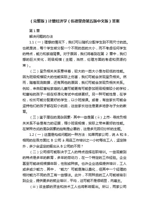
(完整版)计量经济学(伍德里奇第五版中文版)答案第1章解决问题的办法1.1(一)理想的情况下,我们可以随机分配学生到不同尺寸的类。
也就是说,每个学生被分配一个不同的类的大小,而不考虑任何学生的特点,能力和家庭背景。
对于原因,我们将看到在第2章中,我们想的巨大变化,班级规模(主题,当然,伦理方面的考虑和资源约束)。
(二)呈负相关关系意味着,较大的一类大小是与较低的性能。
因为班级规模较大的性能实际上伤害,我们可能会发现呈负相关。
然而,随着观测数据,还有其他的原因,我们可能会发现负相关关系。
例如,来自较富裕家庭的儿童可能更有可能参加班级规模较小的学校,和富裕的孩子一般在标准化考试中成绩更好。
另一种可能性是,在学校,校长可能分配更好的学生,以小班授课。
或者,有些家长可能会坚持他们的孩子都在较小的类,这些家长往往是更多地参与子女的教育。
(三)鉴于潜在的混杂因素- 其中一些是第(ii)上市- 寻找负相关关系不会是有力的证据,缩小班级规模,实际上带来更好的性能。
在某种方式的混杂因素的控制是必要的,这是多元回归分析的主题。
1.2(一)这里是构成问题的一种方法:如果两家公司,说A和B,相同的在各方面比B公司à用品工作培训之一小时每名工人,坚定除外,多少会坚定的输出从B公司的不同?(二)公司很可能取决于工人的特点选择在职培训。
一些观察到的特点是多年的教育,多年的劳动力,在一个特定的工作经验。
企业甚至可能歧视根据年龄,性别或种族。
也许企业选择提供培训,工人或多或少能力,其中,“能力”可能是难以量化,但其中一个经理的相对能力不同的员工有一些想法。
此外,不同种类的工人可能被吸引到企业,提供更多的就业培训,平均,这可能不是很明显,向雇主。
(iii)该金额的资金和技术工人也将影响输出。
所以,两家公司具有完全相同的各类员工一般都会有不同的输出,如果他们使用不同数额的资金或技术。
管理者的素质也有效果。
(iv)无,除非训练量是随机分配。

伍德里奇计量经济学导论课后题计算机操作下载温馨提示:该文档是我店铺精心编制而成,希望大家下载以后,能够帮助大家解决实际的问题。
文档下载后可定制随意修改,请根据实际需要进行相应的调整和使用,谢谢!并且,本店铺为大家提供各种各样类型的实用资料,如教育随笔、日记赏析、句子摘抄、古诗大全、经典美文、话题作文、工作总结、词语解析、文案摘录、其他资料等等,如想了解不同资料格式和写法,敬请关注!Download tips: This document is carefully compiled by the editor. I hope that after you download them, they can help you solve practical problems. The document can be customized and modified after downloading, please adjust and use it according to actual needs, thank you!In addition, our shop provides you with various types of practical materials, such as educational essays, diary appreciation, sentence excerpts, ancient poems, classic articles, topic composition, work summary, word parsing, copy excerpts, other materials and so on, want to know different data formats and writing methods, please pay attention!伍德里奇计量经济学导论课后题计算机操作简介伍德里奇计量经济学导论课程提供了对计量经济学基础概念和方法的全面介绍。
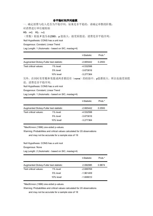
非平稳时间序列建模一.确定消费与收入是否为平稳序列,如果是非平稳的,请确定单整的阶数;对消费进行单位根检验H0:r=1 H1:r<1(常数)检验P值为0.2593,p值很大,接受原假设,消费是非平稳序列。
Null Hypothesis: CONS has a unit rootExogenous: Constant, Linear TrendLag Length: 1 (Automatic - based on SIC, maxlag=4)t-Statistic Prob.*Augmented Dickey-Fuller test statistic -2.665442 0.2593Test critical values: 1% level -4.5325985% level -3.67361610% level -3.277364另外,在同时有常数和变量或两者都没有(none)的检验中,p值都很大,所以也接受原假设,消费是非平稳序列。
Null Hypothesis: CONS has a unit rootExogenous: Constant, Linear TrendLag Length: 1 (Automatic - based on SIC, maxlag=4)t-Statistic Prob.*Augmented Dickey-Fuller test statistic -2.665442 0.2593Test critical values: 1% level -4.5325985% level -3.67361610% level -3.277364*MacKinnon (1996) one-sided p-values.Warning: Probabilities and critical values calculated for 20 observationsand may not be accurate for a sample size of 19Null Hypothesis: CONS has a unit rootExogenous: NoneLag Length: 2 (Automatic - based on SIC, maxlag=4)t-Statistic Prob.*Augmented Dickey-Fuller test statistic 2.082985 0.9874Test critical values: 1% level -2.6997695% level -1.96140910% level -1.606610*MacKinnon (1996) one-sided p-values.Warning: Probabilities and critical values calculated for 20 observationsand may not be accurate for a sample size of 18对消费数据一阶差分后回归的p值仍旧很大,所以仍不平稳形式一:Null Hypothesis: D(CONS) has a unit rootExogenous: ConstantLag Length: 1 (Automatic - based on SIC, maxlag=4)t-Statistic Prob.*Augmented Dickey-Fuller test statistic -2.423252 0.1496 Test critical values: 1% level -3.8573865% level -3.04039110% level -2.660551*MacKinnon (1996) one-sided p-values.Warning: Probabilities and critical values calculated for 20 observationsAnd may not be accurate for a sample size of 18形式二:Null Hypothesis: D(CONS) has a unit rootExogenous: Constant, Linear TrendLag Length: 1 (Automatic - based on SIC, maxlag=4)t-Statistic Prob.*Augmented Dickey-Fuller test statistic -2.757380 0.2283 Test critical values: 1% level -4.5715595% level -3.69081410% level -3.286909*MacKinnon (1996) one-sided p-values.Warning: Probabilities and critical values calculated for 20 observationsAnd may not be accurate for a sample size of 18形式三:Null Hypothesis: D(CONS) has a unit rootExogenous: Constant, Linear TrendLag Length: 1 (Automatic - based on SIC, maxlag=4)t-Statistic Prob.*Augmented Dickey-Fuller test statistic -2.757380 0.2283 Test critical values: 1% level -4.5715595% level -3.69081410% level -3.286909*MacKinnon (1996) one-sided p-values.Warning: Probabilities and critical values calculated for 20 observationsand may not be accurate for a sample size of 18再进行二阶差分检验(none),P值为0.0013,p值很小,消费是二阶非平稳序列。

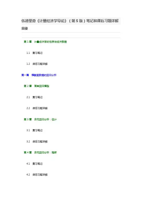
伍德里奇《计量经济学导论》(第5版)笔记和课后习题详解目录第1章计量经济学的性质与经济数据1.1复习笔记1.2课后习题详解第一篇横截面数据的回归分析第2章简单回归模型2.1复习笔记2.2课后习题详解第3章多元回归分析:估计3.1复习笔记3.2课后习题详解第4章多元回归分析:推断4.1复习笔记4.2课后习题详解第5章多元回归分析:OLS的渐近性5.1复习笔记5.2课后习题详解第6章多元回归分析:深入专题6.1复习笔记6.2课后习题详解第7章含有定性信息的多元回归分析:二值(或虚拟)变量7.1复习笔记7.2课后习题详解第8章异方差性8.1复习笔记8.2课后习题详解第9章模型设定和数据问题的深入探讨9.1复习笔记9.2课后习题详解第二篇时间序列数据的回归分析第10章时间序列数据的基本回归分析10.1复习笔记10.2课后习题详解第11章OLS用于时间序列数据的其他问题11.1复习笔记11.2课后习题详解第12章时间序列回归中的序列相关和异方差性12.1复习笔记12.2课后习题详解第三篇高级专题讨论第13章跨时横截面的混合:简单面板数据方法13.1复习笔记13.2课后习题详解第14章高级的面板数据方法14.2课后习题详解第15章工具变量估计与两阶段最小二乘法15.1复习笔记15.2课后习题详解第16章联立方程模型16.1复习笔记16.2课后习题详解第17章限值因变量模型和样本选择纠正17.1复习笔记17.2课后习题详解第18章时间序列高级专题18.1复习笔记18.2课后习题详解第19章一个经验项目的实施19.2课后习题详解本书是伍德里奇《计量经济学导论》(第5版)教材的学习辅导书,主要包括以下内容:(1)整理名校笔记,浓缩内容精华。
每章的复习笔记以伍德里奇所著的《计量经济学导论》(第5版)为主,并结合国内外其他计量经济学经典教材对各章的重难点进行了整理,因此,本书的内容几乎浓缩了经典教材的知识精华。
(2)解析课后习题,提供详尽答案。
《计量经济学》上机实验参考答案实验一:计量经济学软件Eviews 的基本使用;一元线性回归模型的估计、检验和预测;多元线性回归模型的估计、检验和预测(3课时);多元非线性回归模型的估计。
实验设备:个人计算机,计量经济学软件Eviews ,外围设备如U 盘。
实验目的:(1)熟悉Eviews 软件基本使用功能;(2)掌握一元线性回归模型的估计、检验和预测方法;正态性检验;(3)掌握多元线性回归模型的估计、检验和预测方法;(4)掌握多元非线性回归模型的估计方法。
实验方法与原理:Eviews 软件使用,普通最小二乘法(OLS ),拟合优度评价、t 检验、F 检验、J-B 检验、预测原理。
实验要求:(1)熟悉和掌握描述统计和线性回归分析;(2)选择方程进行一元线性回归;(3)选择方程进行多元线性回归;(4)进行经济意义检验、拟合优度评价、参数显著性检验和回归方程显著性检验;(5)掌握被解释变量的点预测和区间预测;(6)估计对数模型、半对数模型、倒数模型、多项式模型模型等非线性回归模型。
实验内容与数据1:表1数据是从某个行业的5个不同的工厂收集的,请回答以下问题:(1)估计这个行业的线性总成本函数:t t x b b y 10ˆˆˆ+=;(2)0ˆb 和1ˆb 的经济含义是什么?;(3)估计产量为10时的总成本。
表1 某行业成本与产量数据 总成本y80 44 51 70 61 产量x 12 4 6 11 8参考答案:(1)总成本函数(标准格式):t t x y25899.427679.26ˆ+= s = (3.211966) (0.367954)t = (8.180904) (11.57462)978098.02=R 462819.2.=E S 404274.1=DW 9719.133=F(2)0ˆb =26.27679为固定成本,即产量为0时的成本;1ˆb =4.25899为边际成本,即产量每增加1单位时,总成本增加了4.25899单位。
过程*describetive statistc*tabstat prate mrate totpart,stat(max min mean p50 sd n)结果stats | prate mrate totpart---------+------------------------------max | 100 4.91 58811min | 3 .01 50mean | 87.36291 .7315124 1354.231p50 | 95.7 .46 276sd | 16.71654 .7795393 4629.265N | 1534 1534 1534过程summarize 全部的加总summarize prate mrate 两个变量summarize sole prate,detail结果summarizeVariable | Obs Mean Std. Dev. Min Max -------------+--------------------------------------------------------prate | 1534 87.36291 16.71654 3 100mrate | 1534 .7315124 .7795393 .01 4.91 totpart | 1534 1354.231 4629.265 50 58811totelg | 1534 1628.535 5370.719 51 70429 age | 1534 13.18123 9.171114 4 51 -------------+--------------------------------------------------------totemp | 1534 3568.495 11217.94 58 144387sole | 1534 .4876141 .5000096 0 1 ltotemp | 1534 6.686034 1.453375 4.060443 11.88025 summarize prate mrateVariable | Obs Mean Std. Dev. Min Max -------------+--------------------------------------------------------prate | 1534 87.36291 16.71654 3 100mrate | 1534 .7315124 .7795393 .01 4.91 summarize sole prate,detail= 1 if 401k is firm's sole plan-------------------------------------------------------------Percentiles Smallest1% 0 05% 0 010% 0 0 Obs 153425% 0 0 Sum of Wgt. 153450% 0 Mean .4876141Largest Std. Dev. .5000096 75% 1 190% 1 1 Variance .2500096 95% 1 1 Skewness .0495589 99% 1 1 Kurtosis 1.002456participation rate, percent-------------------------------------------------------------Percentiles Smallest1% 31.4 35% 53.8 8.810% 62.7 14.9 Obs 1534 25% 78 17.4 Sum of Wgt. 1534 50% 95.7 Mean 87.36291Largest Std. Dev. 16.71654 75% 100 10090% 100 100 Variance 279.4426 95% 100 100 Skewness -1.519626 99% 100 100 Kurtosis 5.258359 .end of do-file过程*cdf*tabulate prate结果累积participati |on rate, |percent | Freq. Percent Cum.------------+-----------------------------------3 | 1 0.07 0.078.8 | 1 0.07 0.1314.9 | 1 0.07 0.2017.4 | 1 0.07 0.2619.3 | 1 0.07 0.3320.1 | 1 0.07 0.3920.6 | 1 0.07 0.4621 | 1 0.07 0.5221.3 | 1 0.07 0.5922.1 | 1 0.07 0.6525.1 | 1 0.07 0.7226.1 | 1 0.07 0.7828.6 | 1 0.07 0.8529 | 1 0.07 0.9130.5 | 1 0.07 0.9831.4 | 1 0.07 1.0433.5 | 1 0.07 1.1734.2 | 1 0.07 1.2435.6 | 1 0.07 1.30 35.8 | 1 0.07 1.37 37 | 1 0.07 1.43 37.5 | 1 0.07 1.5037.7 | 1 0.07 1.5638.1 | 1 0.07 1.63 38.4 | 1 0.07 1.6938.7 | 1 0.07 1.7639.4 | 1 0.07 1.83 39.6 | 1 0.07 1.89 39.8 | 1 0.07 1.9641.5 | 1 0.07 2.0242.1 | 1 0.07 2.09 42.4 | 1 0.07 2.1542.5 | 1 0.07 2.2243.1 | 1 0.07 2.28 43.3 | 1 0.07 2.35 43.6 | 1 0.07 2.4143.8 | 1 0.07 2.4844.1 | 1 0.07 2.54 44.3 | 1 0.07 2.6144.7 | 2 0.13 2.7445.5 | 1 0.07 2.8045.8 | 1 0.07 2.8746.9 | 3 0.20 3.0647.3 | 1 0.07 3.1347.7 | 1 0.07 3.1948.2 | 1 0.07 3.26 48.6 | 2 0.13 3.39 48.8 | 1 0.07 3.4648.9 | 3 0.20 3.6549.2 | 1 0.07 3.72 49.6 | 2 0.13 3.8549.7 | 1 0.07 3.9150 | 1 0.07 3.98 50.2 | 1 0.07 4.04 50.3 | 1 0.07 4.11 50.7 | 1 0.07 4.1750.9 | 2 0.13 4.3051 | 1 0.07 4.37 51.3 | 1 0.07 4.43 51.5 | 1 0.07 4.5051.9 | 1 0.07 4.5652.3 | 1 0.07 4.63 52.4 | 1 0.07 4.6952.7 | 1 0.07 4.7653.1 | 1 0.07 4.8253.7 | 1 0.07 4.9553.8 | 1 0.07 5.0254.1 | 1 0.07 5.08 54.2 | 1 0.07 5.1554.9 | 2 0.13 5.2855.1 | 1 0.07 5.35 55.5 | 1 0.07 5.41 55.7 | 1 0.07 5.4855.9 | 1 0.07 5.5456.2 | 2 0.13 5.67 56.3 | 2 0.13 5.80 56.4 | 1 0.07 5.87 56.7 | 3 0.20 6.0656.8 | 1 0.07 6.1357 | 2 0.13 6.26 57.6 | 2 0.13 6.39 57.7 | 1 0.07 6.4557.8 | 2 0.13 6.5858 | 1 0.07 6.65 58.2 | 3 0.20 6.84 58.3 | 1 0.07 6.91 58.4 | 2 0.13 7.04 58.6 | 2 0.13 7.17 58.7 | 1 0.07 7.2458.8 | 1 0.07 7.3059 | 1 0.07 7.37 59.1 | 2 0.13 7.50 59.2 | 2 0.13 7.63 59.4 | 1 0.07 7.69 59.6 | 3 0.20 7.89 59.8 | 1 0.07 7.9559.9 | 2 0.13 8.0860.1 | 2 0.13 8.21 60.2 | 1 0.07 8.28 60.3 | 1 0.07 8.34 60.4 | 1 0.07 8.41 60.6 | 2 0.13 8.54 60.8 | 2 0.13 8.6760.9 | 2 0.13 8.8061.1 | 1 0.07 8.87 61.2 | 3 0.20 9.06 61.3 | 1 0.07 9.13 61.4 | 1 0.07 9.19 61.5 | 1 0.07 9.26 61.6 | 1 0.07 9.32 61.7 | 2 0.13 9.4561.8 | 2 0.13 9.5862 | 2 0.13 9.71 62.2 | 1 0.07 9.7862.6 | 1 0.07 9.91 62.7 | 2 0.13 10.0462.9 | 2 0.13 10.1763 | 3 0.20 10.37 63.3 | 2 0.13 10.50 63.4 | 1 0.07 10.56 63.6 | 1 0.07 10.6363.7 | 1 0.07 10.6964 | 1 0.07 10.76 64.3 | 1 0.07 10.82 64.4 | 3 0.20 11.02 64.6 | 4 0.26 11.28 64.7 | 1 0.07 11.3464.9 | 2 0.13 11.4765 | 2 0.13 11.60 65.1 | 3 0.20 11.80 65.3 | 1 0.07 11.86 65.5 | 3 0.20 12.06 65.6 | 2 0.13 12.1965.7 | 1 0.07 12.2666.2 | 1 0.07 12.32 66.3 | 2 0.13 12.45 66.5 | 1 0.07 12.52 66.6 | 5 0.33 12.8466.9 | 2 0.13 12.9767 | 1 0.07 13.04 67.1 | 1 0.07 13.10 67.2 | 2 0.13 13.23 67.3 | 3 0.20 13.43 67.6 | 2 0.13 13.5667.8 | 1 0.07 13.6268 | 1 0.07 13.69 68.3 | 1 0.07 13.75 68.5 | 1 0.07 13.82 68.6 | 1 0.07 13.89 68.7 | 3 0.20 14.08 68.8 | 2 0.13 14.2168.9 | 2 0.13 14.3469.2 | 1 0.07 14.41 69.3 | 1 0.07 14.47 69.4 | 1 0.07 14.54 69.6 | 1 0.07 14.60 69.8 | 1 0.07 14.6769.9 | 2 0.13 14.8070 | 2 0.13 14.93 70.2 | 2 0.13 15.06 70.3 | 2 0.13 15.19 70.5 | 1 0.07 15.25 70.6 | 2 0.13 15.3870.9 | 3 0.20 15.6571.1 | 1 0.07 15.71 71.4 | 1 0.07 15.78 71.5 | 1 0.07 15.84 71.6 | 2 0.13 15.97 71.7 | 4 0.26 16.2371.9 | 2 0.13 16.3672 | 2 0.13 16.49 72.1 | 1 0.07 16.56 72.3 | 1 0.07 16.62 72.5 | 2 0.13 16.75 72.6 | 2 0.13 16.88 72.7 | 1 0.07 16.95 72.8 | 2 0.13 17.0872.9 | 3 0.20 17.2873 | 4 0.26 17.54 73.2 | 1 0.07 17.60 73.4 | 3 0.20 17.80 73.5 | 5 0.33 18.12 73.6 | 1 0.07 18.19 73.7 | 3 0.20 18.38 73.8 | 4 0.26 18.6473.9 | 4 0.26 18.9074 | 4 0.26 19.17 74.1 | 2 0.13 19.30 74.3 | 2 0.13 19.43 74.4 | 1 0.07 19.49 74.5 | 1 0.07 19.56 74.6 | 2 0.13 19.69 74.7 | 4 0.26 19.9574.8 | 1 0.07 20.0175 | 1 0.07 20.08 75.1 | 3 0.20 20.27 75.2 | 3 0.20 20.47 75.3 | 7 0.46 20.93 75.4 | 2 0.13 21.06 75.5 | 3 0.20 21.25 75.6 | 1 0.07 21.32 75.7 | 4 0.26 21.58 75.8 | 1 0.07 21.6475.9 | 3 0.20 21.8476.1 | 1 0.07 21.90 76.2 | 1 0.07 21.97 76.3 | 3 0.20 22.16 76.4 | 5 0.33 22.49 76.5 | 3 0.20 22.6976.9 | 2 0.13 22.8277 | 4 0.26 23.08 77.2 | 4 0.26 23.3477.4 | 3 0.20 23.92 77.5 | 2 0.13 24.05 77.6 | 2 0.13 24.19 77.7 | 3 0.20 24.38 77.8 | 1 0.07 24.4577.9 | 3 0.20 24.6478 | 6 0.39 25.03 78.1 | 2 0.13 25.16 78.2 | 2 0.13 25.29 78.3 | 1 0.07 25.36 78.4 | 1 0.07 25.42 78.5 | 4 0.26 25.68 78.6 | 2 0.13 25.81 78.7 | 3 0.20 26.0178.8 | 4 0.26 26.2779 | 4 0.26 26.53 79.1 | 1 0.07 26.60 79.2 | 2 0.13 26.73 79.3 | 5 0.33 27.05 79.4 | 1 0.07 27.12 79.5 | 2 0.13 27.25 79.6 | 1 0.07 27.31 79.7 | 4 0.26 27.57 79.8 | 3 0.20 27.7779.9 | 1 0.07 27.8480 | 2 0.13 27.97 80.1 | 1 0.07 28.03 80.2 | 1 0.07 28.10 80.4 | 2 0.13 28.23 80.5 | 2 0.13 28.36 80.6 | 4 0.26 28.62 80.7 | 2 0.13 28.75 80.8 | 1 0.07 28.8180.9 | 5 0.33 29.1481 | 4 0.26 29.40 81.1 | 2 0.13 29.53 81.2 | 2 0.13 29.66 81.3 | 3 0.20 29.86 81.5 | 2 0.13 29.99 81.6 | 1 0.07 30.05 81.7 | 2 0.13 30.1881.8 | 3 0.20 30.3882 | 2 0.13 30.51 82.1 | 2 0.13 30.64 82.2 | 2 0.13 30.77 82.3 | 1 0.07 30.83 82.5 | 6 0.39 31.23 82.6 | 5 0.33 31.55 82.7 | 2 0.13 31.6882.9 | 2 0.13 31.9483 | 1 0.07 32.01 83.2 | 1 0.07 32.07 83.3 | 2 0.13 32.20 83.4 | 1 0.07 32.27 83.5 | 3 0.20 32.46 83.6 | 2 0.13 32.59 83.7 | 3 0.20 32.79 83.8 | 2 0.13 32.9283.9 | 2 0.13 33.0584 | 1 0.07 33.12 84.1 | 2 0.13 33.25 84.2 | 2 0.13 33.38 84.3 | 3 0.20 33.57 84.5 | 2 0.13 33.70 84.6 | 4 0.26 33.96 84.7 | 2 0.13 34.0984.9 | 4 0.26 34.3585 | 2 0.13 34.49 85.1 | 5 0.33 34.81 85.2 | 2 0.13 34.94 85.3 | 4 0.26 35.20 85.4 | 1 0.07 35.27 85.5 | 3 0.20 35.46 85.6 | 2 0.13 35.59 85.7 | 5 0.33 35.9285.8 | 5 0.33 36.2586 | 2 0.13 36.38 86.1 | 2 0.13 36.51 86.2 | 1 0.07 36.57 86.3 | 4 0.26 36.83 86.4 | 2 0.13 36.96 86.5 | 3 0.20 37.16 86.6 | 1 0.07 37.22 86.7 | 1 0.07 37.29 86.8 | 1 0.07 37.3586.9 | 2 0.13 37.4887 | 2 0.13 37.61 87.1 | 2 0.13 37.74 87.2 | 2 0.13 37.87 87.3 | 2 0.13 38.01 87.4 | 4 0.26 38.27 87.5 | 2 0.13 38.40 87.6 | 4 0.26 38.66 87.7 | 2 0.13 38.79 87.8 | 1 0.07 38.8587.9 | 1 0.07 38.9288 | 3 0.20 39.11 88.1 | 3 0.20 39.3188.3 | 2 0.13 39.63 88.4 | 1 0.07 39.70 88.5 | 2 0.13 39.83 88.6 | 1 0.07 39.9088.8 | 3 0.20 40.0989 | 6 0.39 40.48 89.1 | 2 0.13 40.61 89.2 | 1 0.07 40.68 89.3 | 1 0.07 40.74 89.4 | 3 0.20 40.94 89.5 | 1 0.07 41.00 89.6 | 3 0.20 41.20 89.7 | 2 0.13 41.33 89.8 | 7 0.46 41.7989.9 | 6 0.39 42.1890 | 1 0.07 42.24 90.1 | 2 0.13 42.37 90.2 | 1 0.07 42.44 90.3 | 3 0.20 42.63 90.4 | 2 0.13 42.76 90.5 | 4 0.26 43.02 90.7 | 2 0.13 43.1690.8 | 5 0.33 43.4891 | 1 0.07 43.55 91.1 | 1 0.07 43.61 91.2 | 2 0.13 43.74 91.3 | 1 0.07 43.81 91.4 | 2 0.13 43.94 91.5 | 2 0.13 44.07 91.6 | 5 0.33 44.39 91.7 | 5 0.33 44.72 91.8 | 3 0.20 44.9291.9 | 3 0.20 45.1192 | 2 0.13 45.24 92.1 | 1 0.07 45.31 92.2 | 2 0.13 45.44 92.3 | 3 0.20 45.63 92.4 | 1 0.07 45.70 92.5 | 3 0.20 45.89 92.6 | 3 0.20 46.09 92.7 | 2 0.13 46.22 92.8 | 1 0.07 46.2892.9 | 2 0.13 46.4193 | 2 0.13 46.54 93.1 | 3 0.20 46.74 93.2 | 3 0.20 46.94 93.3 | 3 0.20 47.13 93.4 | 2 0.13 47.26 93.5 | 2 0.13 47.3993.7 | 3 0.20 47.65 93.8 | 2 0.13 47.7893.9 | 4 0.26 48.0494 | 2 0.13 48.17 94.2 | 4 0.26 48.44 94.4 | 4 0.26 48.70 94.5 | 1 0.07 48.76 94.6 | 2 0.13 48.89 94.8 | 2 0.13 49.0294.9 | 1 0.07 49.0995 | 5 0.33 49.41 95.1 | 1 0.07 49.48 95.2 | 1 0.07 49.54 95.3 | 2 0.13 49.67 95.4 | 2 0.13 49.80 95.6 | 2 0.13 49.93 95.7 | 6 0.39 50.33 95.8 | 3 0.20 50.5295.9 | 2 0.13 50.6596 | 3 0.20 50.85 96.1 | 3 0.20 51.04 96.2 | 1 0.07 51.11 96.3 | 3 0.20 51.30 96.4 | 1 0.07 51.37 96.5 | 3 0.20 51.56 96.6 | 1 0.07 51.6396.8 | 3 0.20 51.8397 | 2 0.13 51.96 97.1 | 1 0.07 52.02 97.2 | 2 0.13 52.15 97.4 | 1 0.07 52.22 97.6 | 2 0.13 52.35 97.7 | 3 0.20 52.54 97.8 | 3 0.20 52.7497.9 | 1 0.07 52.8098.1 | 2 0.13 52.93 98.3 | 1 0.07 53.00 98.4 | 1 0.07 53.06 98.5 | 1 0.07 53.13 98.6 | 2 0.13 53.26 98.7 | 1 0.07 53.32 98.8 | 2 0.13 53.4698.9 | 4 0.26 53.7299 | 3 0.20 53.91 99.1 | 4 0.26 54.17 99.2 | 4 0.26 54.43 99.3 | 2 0.13 54.56 99.4 | 1 0.07 54.63 99.5 | 2 0.13 54.7699.6 | 4 0.26 55.0299.7 | 1 0.07 55.0899.8 | 3 0.20 55.2899.9 | 4 0.26 55.54100 | 682 44.46 100.00 ------------+-----------------------------------Total | 1,534 100.00过程*pairwise correlation*pwcorr prate mrate totpart totelgpwcorr prate mrate totpart totelg,sig star(0.05)结果两两相比较| prate mrate totpart totelg -------------+------------------------------------prate | 1.0000mrate | 0.2733 1.0000totpart | 0.0042 0.0186 1.0000totelg | -0.0764 -0.0007 0.9761 1.0000 显著性pwcorr prate mrate totpart totelg,sig star(0.05)| prate mrate totpart totelg -------------+------------------------------------prate | 1.0000||mrate | 0.2733* 1.0000| 0.0000|totpart | 0.0042 0.0186 1.0000| 0.8703 0.4658|totelg | -0.0764* -0.0007 0.9761* 1.0000| 0.0028 0.9770 0.0000|.end of do-file过程*graph*histogram prate,width(5)frequencykdensity pratescatter prate mratetwoway(scatter prate mrate)(qfit prate mrate)graph save graphpractice1结果*graph*. histogram prate,width(5)frequency(bin=20, start=3, width=5). kdensity prate. scatter prate mrate. twoway(scatter prate mrate)(qfit prate mrate). graph save graphpractice1(file graphpractice1.gph saved).end of do-file过程twoway(scatter prate mrate)(lfit prate mrate) graph save graphpractice2graph combine graph1.gph graph2.gph结果 050100012345401k plan match rate participation rate, percentFitted values最新文件仅供参考已改成word文本。